Flux saturation length of sediment transport

Abstract

Sediment transport along the surface drives geophysical phenomena as diverse as wind erosion and dune formation. The main length-scale controlling the dynamics of sediment erosion and deposition is the saturation length $L_{\mathrm{s}}$, which characterizes the flux response to a change in transport conditions. Here we derive, for the first time, an expression predicting $L_{\mathrm{s}}$ as a function of the average sediment velocity under different physical environments. Our expression accounts for both the characteristics of sediment entrainment and the saturation of particle and fluid velocities, and has only two physical parameters which can be estimated directly from independent experiments. We show that our expression is consistent with measurements of $L_{\mathrm{s}}$ in both aeolian and subaqueous transport regimes over at least five orders of magnitude in the ratio of fluid and particle density, including on Mars.

Sediment transport along the surface drives a wide variety of geophysical phenomena, including wind erosion, dust aerosol emission, and the formation of dunes and ripples on ocean floors, river beds, and planetary surfaces Bagnold_1941 ; van_Rijn_1993 ; Garcia_2007 ; Shao_2008 ; Bourke_et_al_2010 ; Kok_et_al_2012 . The primary transport modes are saltation, which consists of particles jumping downstream close to the ground at nearly ballistic trajectories, and creep (grains rolling and sliding along the surface). A critical parameter in sediment transport is the distance needed for the particle flux to adapt to a change in flow conditions, which is characterized by the saturation length, $L_{\mathrm{s}}$. Predicting $L_{\mathrm{s}}$ under given transport conditions remains a long-standing open problem Kok_et_al_2012 ; Andreotti_et_al_2010 ; Franklin_and_Charru_2011 ; Ma_and_Zheng_2011 ; Sauermann_et_al_2001 .

Indeed, $L_{\mathrm{s}}$ partially determines the dynamics of dunes, for instance by dictating the wavelength of the smallest (“elementary”) dunes on a sediment surface Kroy_et_al_2002 ; Fourriere_et_al_2010 and the minimal size of crescent-shaped barchans Kroy_et_al_2002 ; Parteli_et_al_2007 . Moreover, although flux saturation plays a significant role for the evolution of fluvial sediment landscapes Cao_et_al_2012 , morphodynamic models used in hydraulic engineering usually treat $L_{\mathrm{s}}$ as an adjustable parameter He_et_al_2009 . The availability of an accurate theoretical expression predicting $L_{\mathrm{s}}$ for given transport conditions would thus be an important contribution to the planetary, geological and engineering sciences. In this Letter, we present such a theoretical expression for $L_{\mathrm{s}}$. In contrast to previously proposed relations for $L_{\mathrm{s}}$, the expression presented here explicitly accounts for the relevant forces that control the relaxation of particle and fluid velocities, and also incorporates the distinct entrainment mechanisms prevailing in aeolian and subaqueous transport (defined below).

The average momentum of transported grains per unit soil area, the sediment flux $Q$, is defined as $Q=MV$, where $M$ is the mass of sediment in flow per unit soil area, and $V$ is the average particle velocity. Since the fluid loses momentum to accelerate the particles, $Q$ is limited by a steady-state value, the saturated flux $Q_{\mathrm{s}}$. This flux is largely set by the fluid density ${\rho}_{\mathrm{f}}$ and the fluid shear velocity $u_{\ast}$ Bagnold_1941 ; van_Rijn_1993 ; Garcia_2007 ; Shao_2008 ; Kok_et_al_2012 , which is proportional to the mean flow velocity gradient in turbulent boundary layer flow Kok_et_al_2012 . In typical situations, such as on the streamward side of dunes, the deviation of $Q$ from $Q_{\mathrm{s}}$ is small, that is, $|1-Q/Q_{\mathrm{s}}|\ll 1$ Kroy_et_al_2002 ; Sauermann_et_al_2001 ; Duc_and_Rodi_2008 . The rate $\Gamma(Q)$ of the relaxation of $Q$ towards $Q_{\mathrm{s}}$ in the downstream direction ($x$) can thus be approximately written as Sauermann_et_al_2001 ; Duc_and_Rodi_2008 ; Andreotti_et_al_2010 ,

$$\Gamma(Q)={\mathrm{d}Q}/{\mathrm{d}x} \approxeq {\left[{Q_{\mathrm{s}}-Q}\right]}/{L_{\mathrm{s}}},$$ (1)

where $\Gamma$ is Taylor-expanded to first order around $Q=Q_{\mathrm{s}}$ ($\Gamma(Q_{\mathrm{s}})=0$), and the negative inverse Taylor-coefficient gives the saturation length, $L_{\mathrm{s}}$. Flux saturation is controlled by the downstream evolutions of $M$ and $V$ towards their respective steady-state values, $M_{\mathrm{s}}$ and $V_{\mathrm{s}}$. Changes in $M$ with $x$ are controlled by particle entrainment from the sediment bed into the transport layer. In the aeolian regime (dilute fluid such as air), entrainment occurs predominantly through particle impacts Kok_et_al_2012 , whereas in the subaqueous regime (dense fluid such as water) entrainment occurs mainly through fluid lifting van_Rijn_1993 ; Garcia_2007 . On the other hand, the evolution of $V$ towards $V_{\mathrm{s}}$ is mainly controlled by the acceleration of the particles due to fluid drag, and their deceleration due to grain-bed collisions Sauermann_et_al_2001 ; Fourriere_et_al_2010 . We note that the evolution of $V$ is affected by changes in $M$ and vice versa. For instance, an increase of $M$ leads to a decrease in $V$ in the absence of horizontal forces due to conservation of horizontal momentum. For simplicity, previous studies neglected either the saturation of $V$ Sauermann_et_al_2001 ; Charru_2006 or the relaxation of $M$, as well as changes in $V$ due to grain-bed collisions Andreotti_et_al_2010 ; Fourriere_et_al_2010 . Moreover, all previous studies did not account for the relaxation of the fluid velocity ($U$) towards its steady-state value ($U_{\mathrm{s}}$) within the transport layer. This relaxation is driven by changes in the transport-flow feedback resulting from the relaxations of $M$ and $V$. For instance, increasing $V$ reduces the relative velocity $V_{\mathrm{r}}=U-V$ and thus the fluid drag. In turn, as $V_{\mathrm{r}}$ decreases, the amount of momentum transferred from the fluid to the transport layer also decreases, which results in an increase in $U$, whereas an increase in $U$ again increases $V_{\mathrm{r}}$.

In this Letter, we derive a theoretical expression for $L_{\mathrm{s}}$ which encodes all aforementioned relaxation mechanisms. Indeed, since previously proposed relations for $L_{\mathrm{s}}$ neglect some of the interactions that determine $L_{\mathrm{s}}$ Sauermann_et_al_2001 ; Kroy_et_al_2002 ; Andreotti_et_al_2010 ; Fourriere_et_al_2010 , it is uncertain how to adapt these equations to compute $L_{\mathrm{s}}$ in extraterrestrial environments, such as Mars Parteli_et_al_2007 ; Bourke_et_al_2010 ; Kok_et_al_2012 . Our theoretical expression overcomes this problem, since it is valid for arbitrary physical environments for which turbulent fluctuations of the fluid velocity, and thus transport as suspended load Kok_et_al_2012 , can be neglected. For aeolian transport under terrestrial conditions, this regime corresponds to $u_{\ast}\lesssim 4u_{\mathrm{t}}$, where $u_{\mathrm{t}}$ is the threshold $u_{\ast}$ for sustained transport van_Rijn_1993 ; Garcia_2007 ; Kok_et_al_2012 .

We start from the momentum conservation equation for steady ($\partial/\partial t=0$) dilute granular flows Jenkins_and_Richman_1985 ,

$${\partial\rho\langle v_{x}^{2}\rangle}/{\partial x}+{\partial\rho\langle v_{x}v_{z}\rangle}/{\partial z}=\langle f_{x}\rangle,$$ (2)

where $\langle\rangle$ denotes the ensemble average, $\rho$ the mass density, $\mathbf{v}$ the particle velocity, and $\mathbf{f}$ the external body force per unit volume applied on a sediment particle. Here $\mathbf{f}$ incorporates the main external forces acting on the transported particles: drag, gravity, buoyancy, and added mass. The added mass force arises because the speed of the fluid layer immediately surrounding the particle is closely coupled to that of the particle, thereby enhancing the particle’s inertia by a factor $1+0.5s^{-1}$, where $s\!=\!\rho_{\mathrm{p}}/\rho_{\mathrm{f}}$ is the grain-fluid density ratio van_Rijn_1993 . Although this added mass effect is negligible in aeolian transport ($0.5\,s^{-1}\ll 1$), it affects the motion of particles in the subaqueous regime van_Rijn_1993 . Integration of Eq. (2) over the entire transport layer depth ($\int_{0}^{\infty}..\mathrm{d}z$) yields,

$$\frac{\mathrm{d}(c_{v}MV^{2})}{\mathrm{d}x}=\int\limits_{0}^{\infty}\langle f_{x}\rangle\mathrm{d}z+(\rho\langle v_{x}v_{z}\rangle)(0),$$ (3)

where $M=\int_{0}^{\infty}\rho\mathrm{d}z$, $V=\int_{0}^{\infty}\rho\langle v_{x}\rangle\mathrm{d}z/M$, and $c_{v}=\int_{0}^{\infty}\rho\langle v_{x}^{2}\rangle\mathrm{d}z/(MV^{2})$. In Eq. (3), the quantity $(\rho\langle v_{x}v_{z}\rangle)(0)$ gives the difference between the average horizontal momentum of particles impacting onto ($-(\rho_{\downarrow}\langle v_{x}v_{z}\rangle_{\downarrow})(0)$) and leaving ($(\rho_{\uparrow}\langle v_{x}v_{z}\rangle_{\uparrow})(0)$) the sediment bed per unit time and soil area. This momentum change is consequence of the collisions between particles within the sediment bed ($z\leq 0$). Thus, $(\rho\langle v_{x}v_{z}\rangle)(0)$ is an effective frictional force which the soil applies on the transport layer per unit soil area. It is proportional to the normal component of the force which the transport layer exerts onto the sediment bed Garcia_2007 ; Sauermann_et_al_2001 ; Paehtz_et_al_2012 , $(\rho\langle v_{x}v_{z}\rangle)(0)=-\mu gM(s-1)/(s+0.5)$, where $\mu$ is the associated Coulomb friction coefficient, and $g$ the gravitational constant. In order to obtain the momentum conservation equation of the particles within the transport layer from Eq. (3), we first note that $\int\limits_{0}^{\infty}\langle f_{x}^{\mathrm{drag}}\rangle\mathrm{d}z\approx\frac{3M}{4sd}\cdot C_{d}(V_{\mathrm{r}})\cdot V_{\mathrm{r}}^{2}$ Paehtz_et_al_2012 , where $d$ is the mean grain diameter, while $C_{d}(V_{\mathrm{r}})$ is the drag coefficient associated with the fluid drag on transported particles, which is intermediate to fully viscous drag ($C_{d}\propto\nu/[V_{\mathrm{r}}d]$, with $\nu$ standing for the kinematic viscosity) and fully turbulent drag (constant $C_{d}$). By further noting that the change of $c_{v}$ with $x$ is negligible (see Suppl. Mat. Suppl_Mat ), we obtain,

$$c_{v}\frac{\mathrm{d}(MV^{2})}{\mathrm{d}x}=\frac{3M}{4(s+0.5)d}\cdot C_{d}(V_{\mathrm{r}})\cdot V_{\mathrm{r}}^{2}-\frac{s-1}{s+0.5}\mu gM.$$ (4)

Next, we solve Eq. (4) for $\frac{\mathrm{d}V}{\mathrm{d}x}$ thus obtaining an equation of the form $\frac{\mathrm{d}V}{\mathrm{d}x}=\Omega(V)$, and we expand $\Omega(V)$ around saturation, that is, $\Omega(V)\approx\Omega(V_{\mathrm{s}})+(V\!-\!V_{\mathrm{s}})\,{\mathrm{d}\Omega/\mathrm{d}V|_{V_{\mathrm{s}}}}$. By noting that $\Gamma(V)=\frac{\mathrm{d}Q}{\mathrm{d}x}(V)=\left(M(V)+V\frac{\mathrm{d}M(V)}{\mathrm{d}V}\right)\Omega(V)$ and $\Omega(V_{\mathrm{s}})=0$, we obtain $L_{\mathrm{s}}=-(\mathrm{d}\Gamma/\mathrm{d}Q)^{-1}|_{Q=Q_{\mathrm{s}}}=-(\mathrm{d}\Omega/\mathrm{d}V)^{-1}|_{V=V_{\mathrm{s}}}$, which leads to,

$$L_{\mathrm{s}}=(s+0.5)c_{v}{(2+c_{M})V_{\mathrm{s}}}V_{\mathrm{rs}}\mathrm{F}\mathrm{K}\cdot{[\mu(s-1)g]}^{-1},$$ (5)

where $c_{M}=\frac{V_{\mathrm{s}}}{M_{\mathrm{s}}}\frac{\mathrm{d}M}{\mathrm{d}V}(V_{\mathrm{s}})$, and $K=\left(1-\frac{\mathrm{d}U}{\mathrm{d}V}(V_{\mathrm{s}})\right)^{-1}$, while $V_{\mathrm{rs}}$ (the steady-state value of $V_{\mathrm{r}}$) and $F$ are given by,

$$V_{\mathrm{rs}}=\left[{{\sqrt{8\mu(s-1)gd/9+({8\nu}/d)^{2}}-8\nu/d}}\right],\ \ \ {\mbox{and,}}$$ (6)

$$\mathrm{F}={\left[{{V_{\mathrm{rs}}+16\nu/d}}\right]}\cdot{\left[{{2V_{\mathrm{rs}}+16\nu/d}}\right]}^{-1},$$ (7)

respectively. Eqs. (6) and (7) result from using $C_{d}(V_{\mathrm{r}})=\frac{24{\nu}}{{V_{\mathrm{r}}}d}+1.5$ (valid for natural sediment Julien_1995 ). We find that using other reported drag laws only marginally affects the value of $L_{\mathrm{s}}$. Furthermore, we note that in the subaqueous regime $c_{M}\approx 0$, since in this regime $M$ changes within a time-scale which is more than one order of magnitude larger than the time-scale over which $Q$ changes Duran_et_al_2012 . This difference in time-scales implies $V\mathrm{d}M\ll\mathrm{d}Q$ and thus $V\mathrm{d}M\ll M\mathrm{d}V$ in the subaqueous regime. In contrast, in the aeolian regime, $c_{M}\approx 1$ as the total mass of ejected grains upon grain-bed collisions is approximately proportional to the speed of impacting grains Kok_and_Renno_2009 , which yields $M/M_{\mathrm{s}}\approx V/V_{\mathrm{s}}$.

In Eq. (5), the quantity $K$ encodes the effect of the relaxation of the transport-flow feedback, neglected in previous works Sauermann_et_al_2001 ; Andreotti_et_al_2010 ; Charru_2006 . In the subaqueous regime, this transport-flow feedback has a negligible influence on the fluid speed Duran_et_al_2012 (and thus on its relaxation). In this regime, $\frac{\mathrm{d}U}{\mathrm{d}V}(V_{\mathrm{s}})\approx 0$, which yields $K\approx 1$ and thus,

$$L_{\mathrm{s}}^{\mathrm{subaq}} = [2s+1]c_{v}{V_{\mathrm{s}}}V_{\mathrm{rs}}\mathrm{F}\cdot{[\mu(s-1)g]}^{-1}.$$ (8)

In contrast, in the aeolian regime, $U$ scales with the shear velocity at the bed ($u_{\mathrm{b}}$) Paehtz_et_al_2012 ; Duran_et_al_2012 , and thus ${\frac{\mathrm{d}U}{\mathrm{d}V}}(V_{\mathrm{s}})\approx\frac{U_{\mathrm{s}}}{u_{\mathrm{bs}}}\frac{\mathrm{d}u_{\mathrm{b}}}{\mathrm{d}V}(V_{\mathrm{s}})$, where $u_{\mathrm{bs}}$ is the steady-state value of $u_{\mathrm{b}}$. Using the mixing length approximation of inner turbulent boundary layer equations George_2009 , $u_{\mathrm{b}}$ can be expressed as $u_{\mathrm{b}}=u_{\ast}{\left[{1-3MC_{d}(V_{\mathrm{r}})V_{\mathrm{r}}^{2}/(4(s+0.5)d{\rho}_{\mathrm{f}}u_{\ast}^{2})}\right]}^{1/2}$ Duran_et_al_2012 . By using this expression to compute $\frac{\mathrm{d}u_{\mathrm{b}}}{\mathrm{d}V}$ and noting that $u_{\mathrm{bs}}\approx u_{\mathrm{t}}$ Kok_et_al_2012 , we obtain the following expression for $K$,

$$\mathrm{K}=\frac{1+{{{\mathrm{F}}}^{-1}{\left[{(V_{\mathrm{s}}\!+\!V_{\mathrm{rs}})/(2V_{\mathrm{rs}})}\right]}}\cdot[{\left({{u_{\ast}}/{u_{\mathrm{t}}}}\right)}^{2}\!-\!1]}{1+{{\left[{(V_{\mathrm{s}}+V_{\mathrm{rs}})/(2V_{\mathrm{s}})}\right]}}\cdot[{\left({{u_{\ast}}/{u_{\mathrm{t}}}}\right)}^{2}\!-\!1]}.$$ (9)

Using Eq. (9) to compute $K$, $L_{\mathrm{s}}$ in the aeolian regime of transport ($(s+0.5)/(s-1)\approxeq 1$) is then given by,

$$L_{\mathrm{s}}^{\mathrm{aeolian}}=3c_{v}{V_{\mathrm{s}}}V_{\mathrm{rs}}\mathrm{F}\mathrm{K}\cdot{[\mu g]}^{-1}.$$ (10)

We show in Section IV of the Suppl. Mat. Suppl_Mat that Eq. (10) can be approximated by the simpler form of $L_{\mathrm{s}}^{\mathrm{aeolian}}\approx 3c_{v}{V_{\mathrm{s}}^{2}}\cdot{[\mu g]}^{-1}$ in the limit of large $u_{\ast}/u_{\mathrm{t}}$.

Therefore, from our general expression for $L_{\mathrm{s}}$ (Eq. (5)) we obtain two expressions — Eqs. (8) and (10) — which can be used to predict $L_{\mathrm{s}}$ in the subaqueous and aeolian transport regimes, respectively. Both use only two parameters, namely $\mu$ and $c_{v}$, which are estimated from independent measurements. Specifically, ${\mu}$ is estimated from measurements of $M_{\mathrm{s}}$ and $Q_{\mathrm{s}}$ for different values of $u_{\ast}$ in air and under water, while $c_{v}$ is estimated from measurements of the particle velocity distribution Suppl_Mat ; Lajeunesse_et_al_2010 ; Creyssels_et_al_2009 . From these experimental data, we obtain $\mu\approx 1.0$ ($0.5$) and $c_{v}\approx 1.3$ ($1.7$) for the aeolian (subaqueous) regime.

Both Eqs. (8) and (10) are consistent with the behavior of $L_{\mathrm{s}}$ with $u_{\ast}$ observed in experiments. Indeed, $L_{\mathrm{s}}$ mainly depends on $u_{\ast}$ via the average particle velocity, $V_{\mathrm{s}}$. For subaqueous transport, in which $V_{\mathrm{s}}$ is a linear function of $u_{\ast}$, $L_{\mathrm{s}}$ varies linearly with $V_{\mathrm{s}}$ and thus with $u_{\ast}$, which is consistent with experiments Franklin_and_Charru_2011 . In contrast, $V_{\mathrm{s}}$ depends only weakly on $u_{\ast}$ for aeolian transport Kok_et_al_2012 ; Duran_et_al_2012 . Consequently, $L_{\mathrm{s}}$ is only weakly dependent on $u_{\ast}$ in this regime, which is also consistent with experiments Andreotti_et_al_2010 . In fact, when neglecting this weak dependence on $u_{\ast}$, Eq. (10) reduces to $L_{\mathrm{s}}\propto sd$ Andreotti_et_al_2010 ; Fourriere_et_al_2010 in the limit of large particle Reynolds numbers $\sqrt{sgd^{3}}/\nu$ for which $V_{\mathrm{s}}\propto\sqrt{sgd}$ Duran_et_al_2012 . Moreover, we estimate the average particle velocity $V_{\mathrm{s}}$ as a function of $u_{\ast}/u_{\mathrm{t}}$ using well-established theoretical expressions which were validated against experiments of sediment transport in the aeolian or in the subaqueous regime. Specifically, we use the model of Ref. Paehtz_et_al_2012 for obtaining $V_{\mathrm{s}}(u_{\ast}/u_{{\ast}{\mathrm{t}}})$ in the aeolian regime and the model of Ref. Lajeunesse_et_al_2010 for the subaqueous regime Suppl_Mat .

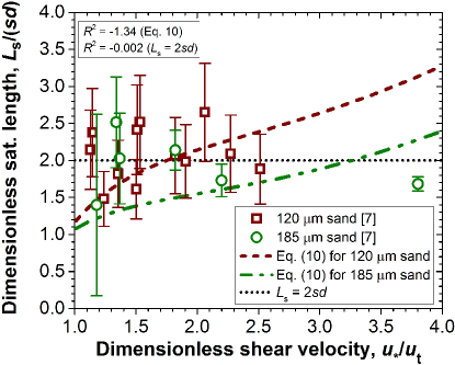
Figure 1: Dimensionless saturation length, $L_{\mathrm{s}}/(sd)$, versus $u_{\ast}/u_{\mathrm{t}}$ for aeolian transport under terrestrial conditions. Brown squares denote estimates of $L_{\mathrm{s}}$ from wind-tunnel measurements ($d=\,120{\mu}$m), while the error bars are due to uncertainties in the measurements of the sediment flux Andreotti_et_al_2010 . Green circles denote $L_{\mathrm{s}}$ obtained from the wavelength of elementary dunes on top of large barchans ($d=185\,{\mu}$m), whereas the error bars contain uncertainties in the dune size Andreotti_et_al_2010 (potential systematic uncertainties Suppl_Mat are not included). The coloured lines represent predicted values of $L_{\mathrm{s}}$ using Eq. (5) for the corresponding experimental conditions ($\rho_{\mathrm{p}}=2650$ kg$/$m³, $\rho_{\mathrm{f}}=1.174$ kg$/$m³ and $\nu=1.59\times 10^{-5}$ m${}^{2}/$s). The dotted horizontal line indicates the prediction of $L_{\mathrm{s}}$ using $L_{\mathrm{s}}=2sd$ Andreotti_et_al_2010 ; Fourriere_et_al_2010 . The upper legend displays the corresponding values of the coefficient of determination, $R^{2}=1-\frac{\sum_{i}\left(L_{\mathrm{s}i}^{\mathrm{measured}}-L_{\mathrm{s}i}^{\mathrm{predicted}}\right)^{2}}{\sum_{i}\left(L_{\mathrm{s}i}^{\mathrm{measured}}-L_{\mathrm{s}}^{\mathrm{mean}}\right)^{2}}$, which is a measure of a theory’s ability to capture variation in data, with $R^{2}$ = 1 corresponding to a perfect fit).

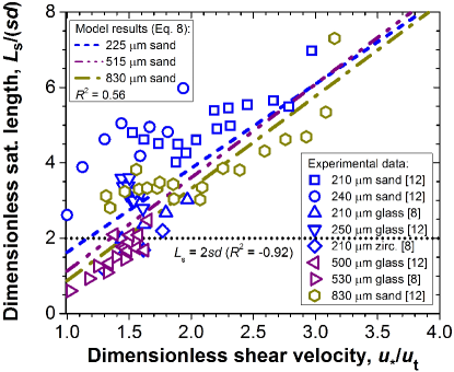
Figure 2: $L_{\mathrm{s}}/(sd)$ versus $u_{\ast}/u_{\mathrm{t}}$ for subaqueous transport. Symbols denote estimates of $L_{\mathrm{s}}$ from the wavelength of elementary dunes Fourriere_et_al_2010 and from the minimal cross-stream width of subaqueous barchans, $W\!\approx\!12\,L_{\mathrm{s}}$ Franklin_and_Charru_2011 . The coloured lines denote predicted values of $L_{\mathrm{s}}$ using Eq. (5) for subaqueous transport of sand (${\rho}_{\mathrm{p}}\!=\!2650\,$kg$/$m³, $\rho_{\mathrm{f}}\!=\!10^{3}\,$kg$/$m³ and $\nu\!=\!10^{-6}\,$m${}^{2}/$s), with grain sizes roughly matching those used in the experiments. The dotted horizontal line indicates the prediction of $L_{\mathrm{s}}$ using the scaling $L_{\mathrm{s}}=2sd$ Andreotti_et_al_2010 ; Fourriere_et_al_2010 . The values of $R^{2}$ (coefficient of determination) for both expressions are also shown.

The squares in Fig. 1 denote wind tunnel measurements of $L_{\mathrm{s}}$ for different values of $u_{\ast}$. These data were obtained by fitting Eq. (1) to the downstream evolution of the sediment flux, $Q(x)$, close to equilibrium Andreotti_et_al_2010 . Further estimates of $L_{\mathrm{s}}$ for aeolian transport under terrestrial conditions have been obtained from the wavelength ($\lambda$) of elementary dunes on top of large barchans Andreotti_et_al_2010 ; Suppl_Mat . These estimates correspond to the circles in Fig. 1, whereas the coloured lines in this figure denote $L_{\mathrm{s}}/(sd)$ versus $u_{\ast}/u_{\mathrm{t}}$ predicted by Eq. (10). As we can see in Fig. 1, in spite of the scatter in the data, Eq. (10) yields reasonable agreement with the experimental data without requiring any fitting to these data. In contrast, the scaling $L_{\mathrm{s}}=2sd$ Andreotti_et_al_2010 ; Fourriere_et_al_2010 was obtained from a fit to the data displayed in Fig. 1. Moreover, Fig. 2 shows values of $L_{\mathrm{s}}$ estimated from experiments on subaqueous transport under different shear velocities (symbols). These estimates were obtained from measurements of $\lambda$ Fourriere_et_al_2010 ; Langlois_and_Valance_2007 and from the minimal cross-stream width, $W\approx 12L_{\mathrm{s}}$ Parteli_et_al_2007 , of barchans in a water flume Franklin_and_Charru_2011 . The coloured lines show the behavior of $L_{\mathrm{s}}$ with $u_{\ast}$ as predicted from Eq. (8) for subaqueous sand transport. We note that Eq. (8) is the first expression for $L_{\mathrm{s}}$ that shows good agreement with measurements of $L_{\mathrm{s}}$ under water. Indeed, the scaling relation $L_{\mathrm{s}}=2sd$ does not capture the increasing trend of $L_{\mathrm{s}}$ with $u_{\ast}/u_{\mathrm{t}}$ evident from the experimental data.

An excellent laboratory for further testing our model is the surface of Mars, where the ratio of grain to fluid density ($s$) is about two orders of magnitude larger than on Earth. We estimate the Martian $L_{\mathrm{s}}$ from reported values of the minimal crosswind width $W$ of barchans at Arkhangelsky crater in the southern highlands and at a dune field near the north pole Parteli_et_al_2007 ; Suppl_Mat . However, using Eq. (10) to predict $L_{\mathrm{s}}$ on Mars is difficult because both the grain size $d$ and the typical shear velocity $u_{{\ast}{\mathrm{typ}}}$ for which the dunes were formed are poorly known. Indeed, we need to know both quantities to calculate $V_{\mathrm{s}}$ Paehtz_et_al_2012 . We thus predict the Martian $L_{\mathrm{s}}$ using a range of plausible values of $d$ and $u_{{\ast}{\mathrm{typ}}}$. Specifically, we assume $d$ to lie in the broad range of $100-600\,{\mu}$m based on recent studies Bourke_et_al_2010 . Estimating $u_{{\ast}{\mathrm{typ}}}$ on Mars is also difficult, both because of the scarcity of wind speed measurements Sullivan_et_al_2000 , and because the threshold $u_{\ast}$ required to initiate transport ($u_{\mathrm{ft}}$) likely exceeds $u_{\mathrm{t}}$ by up to a factor of $\sim 10$ Kok_et_al_2012 ; Paehtz_et_al_2012 ; Kok_2010 . We therefore calculate $L_{\mathrm{s}}$ for two separate estimates of $u_{{\ast}{\mathrm{typ}}}$: the first using $u_{{\ast}{\mathrm{typ}}}=u_{\mathrm{ft}}$, consistent with previous studies Parteli_et_al_2007 ; Sullivan_et_al_2005 , and the second calculating $u_{{\ast}{\mathrm{typ}}}$ based on the wind speed probability distribution measured at the Viking 2 landing site Suppl_Mat , which results in an estimate of $u_{{\ast}{\mathrm{typ}}}$ closer to $u_{\mathrm{t}}$. Fig. 3 shows that the values of $L_{\mathrm{s}}$ predicted with either of these estimates are consistent with those estimated from the minimal barchan width. This good agreement suggests that the previously noted overestimation of the minimal size of Martian dunes Kroy_et_al_2005 is largely resolved by accounting for the low Martian value of $u_{\mathrm{t}}/u_{\mathrm{ft}}$ Paehtz_et_al_2012 and the proportionally lower value of the particle speed $V_{\mathrm{s}}$, as hypothesized in Ref. Kok_2010 . Indeed, the scaling $L_{\mathrm{s}}=2sd$ (inset of Fig. 3) requires $d\approx 29\mu$m and $d\approx 40\mu$m to be consistent with $L_{\mathrm{s}}$ for the north polar and Arkhangelsky dune fields, respectively. However, such particles are most likely transported as suspended load on Mars Sullivan_et_al_2005 , as they are on Earth Shao_2008 .

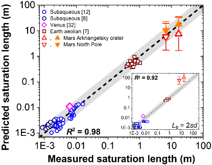
Figure 3: Comparison of measured and predicted values of $L_{\mathrm{s}}$ for various environments; the grey shading denotes agreement between measurements and Eqs. (10) and (8) within a factor of two. Aeolian and subaqueous data were obtained as described in Figs. 1 and 2. For Venus, $L_{\mathrm{s}}$ was estimated from the wavelength of elementary dunes Suppl_Mat . For Mars, $L_{\mathrm{s}}$ was derived from estimates of the minimal size of barchans in two Martian dune fields Suppl_Mat , and plotted against the predicted $L_{\mathrm{s}}$ for a range of plausible dune particle sizes ($d=100-600\,{\mu}$m Bourke_et_al_2010 ) and for two separate estimates of $u_{{\ast}{\mathrm{typ}}}$ (see text). The error bars denote the range in predicted $L_{\mathrm{s}}$ arising from the range in $d$ Bourke_et_al_2010 , and the symbols denote the geometric mean. The filled orange symbols use $u_{{\ast}{\mathrm{typ}}}=u_{\mathrm{ft}}$ Parteli_et_al_2007 ; Sullivan_et_al_2005 , while the open red symbols use the $u_{{\ast}{\mathrm{typ}}}$ calculated from Viking 2 wind speed measurements Suppl_Mat . The inset shows measured and predicted values of $L_{\mathrm{s}}$ for the same conditions as in the main plot, but using $L_{\mathrm{s}}=2sd$ Andreotti_et_al_2010 ; Fourriere_et_al_2010 . Values of $R^{2}$ (coefficient of determination) in each plot were calculated in log10-space such that each data point was weighted equally.

Finally, Fig. 3 also compares Eq. (8) to measurements of $L_{\mathrm{s}}$ for Venusian transport, which have been estimated from the wavelength of elementary dunes produced in a wind-tunnel mimicking the Venusian atmosphere Marshall_and_Greeley_1992 .

In conclusion, Eq. (5) is the first expression capable of quantitatively reproducing measurements of the saturation length $L_{\mathrm{s}}$ under different flow conditions in both air and under water, and is in agreement with measurements over at least 5 orders of magnitude of variation in the sediment to fluid density ratio. The future application of this expression thus has the potential to provide important contributions to calculate sediment transport, the response of saltation-driven wind erosion and dust aerosol emission to turbulent wind fluctuations, and the dynamics of sediment-composed landscapes under water, on Earth’s surface and on other planetary bodies.

We acknowledge support from grants NSFC 41350110226, NSFC 41376095, ETH-10-09-2, NSF AGS 1137716, and DFG through the Cluster of Excellence “Engineering of Advanced Materials”. We thank Miller Mendoza and Robert Sullivan for discussions, and Jeffery Hollingsworth for providing us with the pressure and temperature at the Martian dune fields.

References

- (1) R. A. Bagnold, The physics of blown sand and desert dunes (Methuen, London, 1941).
- (2) L. C. van Rijn, Principles of sediment transport in rivers, estuaries and coastal seas (Aqua Publications, Amsterdam, 1993).
- (3) M. H. Garcia, Sedimentation engineering: processes, measurements, modeling and practice (ASCE, Reston, Va., 2007).
- (4) Y. Shao, Physics and modelling of wind erosion (Kluwer Academic, Dordrecht, 2008).
- (5) M. C. Bourke et al. Geomorphology 121, 1 (2010).
- (6) O. Durán, P. Claudin and B. Andreotti, Aeolian Research 3, 243 (2011); J. F. Kok, et al., Rep. Progr. Phys. 75, 106901 (2012).
- (7) B. Andreotti, P. Claudin and O. Pouliquen, Geomorphology 123, 343 (2010).
- (8) E. M. Franklin and F. Charru, J. Fluid Mech. 675, 199 (2011).
- (9) G. S. Ma and X. J. Zheng, Eur. Phys. J. E 34, 1 (2011).
- (10) G. Sauermann, K. Kroy and H. J. Herrmann, Phys. Rev. E 64, 031305 (2001).
- (11) K. Kroy, G. Sauermann and H. J. Herrmann, Phys. Rev. Lett. 88, 054301 (2002).
- (12) A. Fourrière, P. Claudin and B. Andreotti, J. Fluid Mech. 649, 287 (2010).
- (13) E. J. R. Parteli, O. Durán and H. J. Herrmann, Phys. Rev. E 75, 011301 (2007); E. J. R. Parteli and H. J. Herrmann, Phys. Rev. E 76, 041307 (2007).
- (14) Z. Cao et al., Proc. ICE. Water Management 165, 193211 (2012).
- (15) Z. He, W. Wu and S. Wang, J. Hydr. Eng. 135, 1028 (2009); P. Hu, et al., J. Hydrol. (Amst.) 464, 41 (2012).
- (16) B. M. Duc and W. Rodi, J. Hydr. Eng. 134, 367 (2008).
- (17) F. Charru, Phys. Fluids 18, 121508 (2006).
- (18) J. T. Jenkins and M. W. Richman, Arch. Ration. Mech. Anal. 87, 355 (1985).
- (19) T. Pähtz, J. F. Kok and H. J. Herrmann, New J. Phys. 14, 043035 (2012).
- (20) See Supplemental Material for a description of how we estimated the model parameters and , the average sediment velocity , and the saturation length of sediment transport from the size of dunes under water and on planetary bodies.
- (21) P. Y. Julien, Erosion and Sedimentation (Press Syndicate of the University of Cambridge, 1995).
- (22) O. Durán, B. Andreotti and P. Claudin, Phys. Fluids 24, 103306 (2012).
- (23) J. F. Kok and N. O. Renno, J. Geophys. Res. 114, D17204 (2009).
- (24) W. K. George, Lectures in turbulence for the 21st Century (Chalmers University Goethenborg), pp. 125-126 (2009).
- (25) E. Lajeunesse, L. Malverti and F. Charru, J. Geophys. Res. 115, F04001 (2010).
- (26) M. Creyssels et al., J. Fluid Mech. 625, 47 (2009); K. R. Rasmussen and M. Sørensen, J. Geophys. Res. 113, F02S12 (2008).
- (27) J. H. Baas, Sedimentology 46, 123138 (1999); V. Langlois and A. Valance, Eur. Phys. J. E 22, 201 (2007).
- (28) L. Sutton, C. B. Leovy and J. E. Tillman, J. Atmos. Sci. 35, 2346 (1978); R. Sullivan et al., J. Geophys. Res. 105, 24547 (2000); C. Holstein-Rathlou et al., J. Geophys. Res. 115, E00E18 (2010).
- (29) J. F. Kok, Phys. Rev. Lett. 104, 074502 (2010); Geophys. Res. Lett. 37, L12202 (2010).
- (30) R. E. Arvidson et al., Science 222, 463 (1983); H. J. Moore, J. Geophys. Res. 90, 163 (1985); R. Sullivan, et al., Nature 436, 58 (2005).
- (31) K. Kroy, S. Fischer and B. Obermayer, J. Phys.: Condens. Matter 17, S1299 (2005).
- (32) J. R. Marshall and R. Greeley, J. Geophys. Res. 97, 1007 (1992).