Some large deviations in Kingman’s coalescent

Abstract

Kingman’s coalescent is a random tree that arises from classical population genetic models such as the Moran model. The individuals alive in these models correspond to the leaves in the tree and the following two laws of large numbers concerning the structure of the tree-top are well-known: (i) The (shortest) distance, denoted by $T_{n}$, from the tree-top to the level when there are $n$ lines in the tree satisfies $nT_{n}\xrightarrow{n\to\infty}2$ almost surely; (ii) At time $T_{n}$, the population is naturally partitioned in exactly $n$ families where individuals belong to the same family if they have a common ancestor at time $T_{n}$ in the past. If $F_{i,n}$ denotes the size of the $i$th family, then $n(F_{1,n}^{2}+\cdots+F_{n,n}^{2})\xrightarrow{n\to\infty}2$ almost surely. For both laws of large numbers we prove corresponding large deviations results. For (i), the rate of the large deviations is $n$ and we can give the rate function explicitly. For (ii), the rate is $n$ for downwards deviations and $\sqrt{n}$ for upwards deviations. For both cases we give the exact rate function.

1 Introduction

Kingman’s coalescent is a random tree introduced by Kingman (1982) as the genealogy arising in large population genetic models. It has infinitely many leaves and is usually constructed from leaves to the root as follows: given that there are $k$ lines in the tree, after some exponential time with rate $\binom{k}{2}$, two lines are chosen uniformly and merged to one line, leaving the tree with $k-1$ lines. Due to the quadratic rate $\binom{k}{2}$ the tree immediately comes down from infinitely to finitely many leaves (Donnelly, 1991). Since the seminal paper by Pitman (1999) this random tree has been generalized to other infinite trees arising in population genetics models.

For the Kingman coalescent some laws of large numbers and central limit theorems have been proved. They are nicely summarized in Aldous (1999), Chapter 4.2; see also Proposition 2.1 below. For $\varepsilon>0$ let $N_{\varepsilon}$ denote the number of lines time $\varepsilon$ in the past. Then, since the Kingman coalescent immediately comes down from infinity, $N_{\varepsilon}$ is finite. Furthermore it is approximately $2/\varepsilon$. Equivalently, the time $T_{n}$ it takes the coalescent to go from infinitely many lines to $n$ lines is approximately $2/n$ for large $n$. Going to the fine structure, at time $T_{n}$ the infinite population is decomposed in $n$ families (whose joint distribution is exchangeable) and every leaf in the tree belongs to exactly one of the $n$ families whose frequencies are denoted by $F_{1,n},\dots,F_{n,n}$. It is known that for large $n$ a randomly chosen $F_{i,n}$ is approximately exponentially distributed with mean $1/n$. This translates into several laws of large numbers; see e.g. (35) in Aldous (1999). In particular the probability of picking (from the initial infinite population) two leaves that belong to the same family, given by $F_{1,n}^{2}+\dots+F_{n,n}^{2}$, is approximately $2/n$.

The main goal of the present paper is to study the corresponding large deviations results. To the best of our knowledge, except for Angel et al. (2012), cf. Remark 2.6, results in this direction are not present in the literature. We formulate our results in the next section. Theorem 1 gives a full large deviation principle for the distributions of $nT_{n}$. The proof, given in Section 3, is an application of the Gärtner-Ellis Theorem. As a byproduct, we derive a large deviation principle for the distributions of $\varepsilon N_{\varepsilon}$ in Corollary 2.4. Large deviations of $n(F_{1,n}^{2}+\dots+F_{n,n}^{2})$ are considered in Theorem 2 and exact rate functions for downwards and upwards deviations are given. The proof is given in Section 4.2. For the upward deviations we use a variant of Cramér’s theorem for heavy-tailed random variables; see e.g. Gantert et al. (2014). For the downward deviations we use a connection to self-normalized large deviations; see Shao (1997). This connection was pointed out to us by Alain Rouault and Nina Gantert. Since the rate function for downward deviations is hard to treat analytically we provide in Theorem 3 a simple lower bound. The proof of that bound is given in Section 4.3.

2 Main results

The Kingman coalescent can be seen as a discrete graph, more precisely a discrete tree with infinitely many leaves. Let $S_{2},S_{3},\dots$ be independent exponentially distributed variables with mean $1$. Then the Kingman coalescent tree can be constructed from the root to the leaves as follows.

1. Start the tree with two lines from the root.

2. For $k\geq 2$ the tree stays with $k$ lines for the amount of time $S_{k}/\binom{k}{2}$. After that time one of the $k$ lines is randomly chosen. This line splits in two so that the number of lines jumps from $k$ to $k+1$.

3. Stop upon reaching infinitely many lines, which happens after (the almost surely finite) time $T_{1}\coloneqq\sum_{k=2}^{\infty}S_{k}/\binom{k}{2}$.

The random variable $T_{1}$ is the total tree height. Alternatively, $T_{1}$ is the time to the most recent common ancestor (MRCA) of the infinite population (of leaves). Counted from the top of the tree at time $\varepsilon>0$ a random number $N_{\varepsilon}$ of active lines in the Kingman tree is present, i.e.

$$N_{\varepsilon}\coloneqq\inf\{n:T_{n}<\varepsilon\}\qquad\text{for}\qquad T_{n}\coloneqq\sum_{k=n+1}^{\infty}\frac{S_{k}}{\binom{k}{2}}.$$ (2.1)

At time $T_{n}$ every leaf belongs to one of $n$ disjoint families and all members of each such family stem from the same line at time $T_{n}$. Let us denote the frequencies of these families (which exist due to exchangeability by deFinetti’s Theorem) by $F_{1,n},\dots,F_{n,n}$. The following results are well known (see Aldous (1999) for (2.2) and (2.3) and Evans (2000) for (2.4); proofs can also be found in Depperschmidt et al. (2013).)

Proposition 2.1 (Laws of large numbers).

Let $(T_{n})_{n=1,2,\dots}$, $(N_{\varepsilon})_{\varepsilon>0}$ and $(F_{1,n},\dots,F_{n,n})_{n=1,2,\dots}$ be as above. Then

$$nT_{n} \xrightarrow{n\to\infty}2\quad\text{almost surely,}$$ (2.2)

$$\varepsilon N_{\varepsilon} \xrightarrow{\varepsilon\to 0}2\quad\text{almost surely,}$$ (2.3)

and

$$n\sum_{k=1}^{n}F_{k,n}^{2} \xrightarrow{n\to\infty}2\quad\text{almost surely.}$$ (2.4)

Remark 2.2 (Interpretation of (2.4)).

We note that the left hand side of (2.4) has the interpretation of a homozygosity by descent in the following sense: when picking two leaves from the tree at time $0$, the probability that both share a common ancestor at time $T_{n}$ is $\sum_{k=1}^{n}F_{k,n}^{2}$. Then, the law of large number states that the homozygosity by descent at time $T_{n}$ is approximately $2/n$ for large $n$.

In the present paper we are interested in large deviations results corresponding to the statements of Proposition 2.1. We start with large deviations connected with (2.2). First we introduce some notation. For $n=1,2,\dots$ let $\mu_{n}$ denote the distribution of $nT_{n}$, i.e. $\mu_{n}(\,\cdot\,)=\mathbf{P}(nT_{n}\in\,\cdot\,)$. Furthermore we denote by $\mathcal{B}(\mathbb{R})$ the Borel $\sigma$-algebra on $\mathbbm{R}$ and for $\Gamma\in\mathcal{B}(\mathbb{R})$ we denote by $\Gamma^{\circ}$ the interior and by $\mkern 1.5mu\overline{\mkern-1.5mu\Gamma\mkern-1.5mu}\mkern 1.5mu$ the closure of $\Gamma$. For $x>0$, let $t_{x}<1$ be the unique solution of the equation $x=f(t)$, where the continuous and increasing function $f:(-\infty,1)\to(0,\infty)$ is defined by (see Figure 1 for a plot)

$$f(t)\coloneqq\begin{cases}\displaystyle\frac{1}{\sqrt{t}}\log\frac{1+\sqrt{t}}{1-\sqrt{t}}&:\;0<t<1,\\[8.61108pt] 2&:\;t=0,\\[8.61108pt] \displaystyle\frac{2}{\sqrt{|t|}}\arctan\sqrt{|t|}&:\;t<0.\end{cases}$$ (2.5)

The proof of the following theorem is given in Section 3.1.

Theorem 1 (LDP for $(\mu_{n})_{n=1,2,\dots}$).

The sequence $(\mu_{n})_{n=1,2,\dots}$ satisfies a large deviation principle with scale $n$ and good rate function $I$ given by

$$I(x)\coloneqq\begin{cases}\displaystyle\frac{t_{x}}{2}x+\int_{1}^{\infty}\log\Big{(}1-\frac{t_{x}}{y^{2}}\Big{)}\,dy&:\;x>0,\\[12.91663pt] \infty&:\;x\leq 0.\end{cases}$$ (2.6)

In other words, for any $\Gamma\in\mathcal{B}(\mathbb{R})$ we have

$$-\inf_{x\in\Gamma^{\circ}}I(x)\leq\liminf_{n\to\infty}\frac{1}{n}\log\mu_{n}(\Gamma)\leq\limsup_{n\to\infty}\frac{1}{n}\log\mu_{n}(\Gamma)\leq-\inf_{x\in\mkern 1.5mu\overline{\mkern-1.5mu\Gamma\mkern-1.5mu}\mkern 1.5mu}I(x).$$

Figure 1: This figure displays the functions $f$ and $I$ from (2.5) and (2.6), respectively.

Remark 2.3 (Interpretation).

Both, the function $f$ from (2.5) and $I$ from (2.6) are plotted in Figure 1. The minimum of the rate function is attained at $x=2$. This fact is clear from the law of large numbers, (2.2). In addition, $I(x)=\infty$ for $x\leq 0$ because $nT_{n}>0$ almost surely.

Let us now have a closer look at the behaviour of $I(x)$ for $x$ near $0$ and for large $x$. Since $2\arctan(t)\xrightarrow{t\to\infty}\pi$, we have that $\sqrt{|t_{x}|}x\xrightarrow{x\downarrow 0}\pi$, and hence, $t_{x}\stackrel{{\scriptstyle x\downarrow 0}}{{\approx}}-\frac{\pi^{2}}{x^{2}}$. In this case,

$$xI(x) \stackrel{{\scriptstyle x\downarrow 0}}{{\approx}}-\frac{\pi^{2}}{2}+x\int_{1}^{\infty}\log\Big{(}1+\frac{\pi^{2}}{x^{2}y^{2}}\Big{)}dy$$ (2.7)

$$\stackrel{{\scriptstyle x\downarrow 0}}{{\approx}}-\frac{\pi^{2}}{2}+\pi\int_{0}^{\infty}\log\Big{(}1+\frac{1}{z^{2}}\Big{)}dz=\frac{\pi^{2}}{2},$$

where the last equality follows from $\int_{0}^{\infty}\log(1+1/z^{2})dz=\pi$. To understand the behaviour for large $x$, note that since

$$f(t)\stackrel{{\scriptstyle t\uparrow 1}}{{\approx}}\log 2-\log(1-\sqrt{t}),$$

for $x\to\infty$ we have $2/(1-\sqrt{t_{x}})\approx e^{x}$ and in particular $t_{x}\approx(1-2e^{-x})^{2}\approx 1$. It follows

$$\frac{I(x)}{x}\stackrel{{\scriptstyle x\to\infty}}{{\approx}}\frac{1}{2}+\frac{1}{x}\int_{1}^{\infty}\log(1-1/y^{2})\,dy\stackrel{{\scriptstyle x\to\infty}}{{\approx}}\frac{1}{2}.$$

Note that (2.2) and (2.3) are equivalent. Indeed, $\{T_{n}\geq\varepsilon\}=\{N_{\varepsilon}\geq n\}$ (this also holds with $\geq$ replaced by $\leq$) by construction, and $T_{n}\downarrow 0$ as $n\to\infty$ and $N_{\varepsilon}\uparrow\infty$ as $\varepsilon\to 0$. Hence, Theorem 1 translates into a large deviation principle for $\varepsilon N_{\varepsilon}$. In the following we denote by $\nu_{\varepsilon}$ the distribution of $\varepsilon N_{\varepsilon}$, i.e. $\nu_{\varepsilon}(\,\cdot\,)=\mathbf{P}(\varepsilon N_{\varepsilon}\in\,\cdot\,)$. The proof of the next result is given in Section 3.2; see Figure 2 for a plot of the rate function $\widehat{I}$.

Corollary 2.4 (LDP for $(\nu_{\varepsilon})_{\varepsilon>0}$).

For $\varepsilon\downarrow 0$ the family $(\nu_{\varepsilon})_{\varepsilon>0}$ satisfies a large deviation principle with scale $1/\varepsilon$ and good rate function $\widehat{I}$ given by

$$\widehat{I}(x)=\begin{cases}xI(x)&:\,x>0,\\[6.45831pt] \displaystyle\frac{\pi^{2}}{2}&:\,x=0,\\[6.45831pt] \infty&:\,x<0,\end{cases}$$ (2.8)

with $I$ from (2.6). In particular, for $\Gamma\in\mathcal{B}(\mathbb{R})$ we have

$$-\inf_{x\in\Gamma^{\circ}}\widehat{I}(x)\leq\liminf_{\varepsilon\to 0}\varepsilon\log\nu_{\varepsilon}(\Gamma)\leq\limsup_{\varepsilon\to 0}\varepsilon\log\nu_{\varepsilon}(\Gamma)\leq-\inf_{x\in\mkern 1.5mu\overline{\mkern-1.5mu\Gamma\mkern-1.5mu}\mkern 1.5mu}\widehat{I}(x).$$

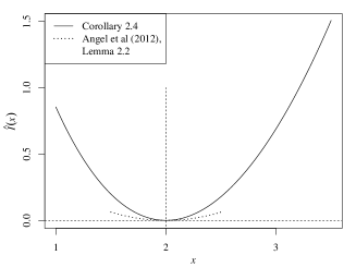
Figure 2: The figure on the left shows the rate function $\widehat{I}$ from Corollary 2.4. The figure on the right is a comparison of $\widehat{I}$ with the lower bound obtained from Angel et al. (2012).

Remark 2.5 (The full distribution of $N_{\varepsilon}$).

The distributions $\nu_{\varepsilon},\varepsilon>0$ (as well as $\mu_{n},n=1,2,\dots$) have been described explicitely in the literature. Tavaré (1984), Section 6, gives

$$\mathbf{P}(N_{\varepsilon}=n)=\sum_{k=n}^{\infty}e^{-\binom{k}{2}\varepsilon}\frac{(-1)^{k-n}(2k-1)\cdot n\cdots(n+k-2)}{n!(k-n)!}.$$

In principle, this formula must also give the large deviations for the measures $\nu_{\varepsilon}$, but this does not seem straight-forward.

Remark 2.6 (The rate function $\widehat{I}$ and comparison with Angel et al. (2012)).

Although the main goal of Angel et al. (2012) was the analysis of spatial $\Lambda$-coalescents, they also provide some large deviations bounds on Kingman’s coalescent. These bounds are mainly based on Markov inequality. Precisely, in Lemma 2.2 in Angel et al. (2012) it is shown that for $0<x<\tfrac{1}{2}$

$$\mathbf{P}(|\varepsilon N_{\varepsilon}-2|>x)<e^{-\frac{x^{2}}{4\varepsilon}}$$

and therefore

$$\limsup_{\varepsilon\to 0}\varepsilon\log\mathbf{P}(|\varepsilon N_{\varepsilon}-2|>x)\leq-\frac{x^{2}}{4}.$$

In the neighbourhood of $2$ the last inequality translates easily into a bound for the rate function $\widehat{I}$ from (2.8); see Figure 2. Namely, for $x\in(1.5,2.5)$ we have

$$\widehat{I}(x)\geq\frac{(x-2)^{2}}{4}.$$

Next, we state some large deviations results connected to (2.4). For

$$W_{n}\coloneqq n\sum_{k=1}^{n}F_{k,n}^{2}$$

we know from (2.4) that $W_{n}\xrightarrow{n\to\infty}2$ holds almost surely. The proof of this result is based on the well-known fact (see e.g. Section 5 in Kingman (1982)) that the distribution of $W_{n}$ can be derived using uniform order statistics: Let $U_{1},\dots,U_{n-1}$ be independent and uniformly distributed on $[0,1]$, and $0<U_{(1)}<\cdots<U_{(n-1)}<1$ be their order statistics. Additionally, let $R_{1},\dots,R_{n}$ be independent exponentially distributed random variables with mean $1$. Then,

$$(F_{1,n},\dots,F_{n,n}) \stackrel{{\scriptstyle d}}{{=}}\bigl{(}U_{(1)},U_{(2)}-U_{(1)},\dots,U_{(n-1)}-U_{(n-2)},1-U_{(n-1)}\bigr{)}$$ (2.9)

$$\stackrel{{\scriptstyle d}}{{=}}\Big{(}\frac{R_{1}}{\sum_{j=1}^{n}R_{j}},\dots,\frac{R_{n}}{\sum_{j=1}^{n}R_{j}}\Big{)}.$$

Here the second equality in distribution is one of the well known representations of uniform spacings; see e.g. Section 4.1 in Pyke (1965). It follows

$$W_{n}\stackrel{{\scriptstyle d}}{{=}}n\frac{\sum_{k=1}^{n}R_{k}^{2}}{\Big{(}\sum_{j=1}^{n}R_{j}\Big{)}^{2}}=\frac{\frac{1}{n}\sum_{k=1}^{n}R_{k}^{2}}{\Big{(}\frac{1}{n}\sum_{j=1}^{n}R_{j}\Big{)}^{2}}.$$ (2.10)

We will use this representation to obtain large deviations results for $W_{n}$. In particular we show that upwards large deviations of $W_{n}$ are on the scale $\sqrt{n}$ while downwards large deviations are on the scale $n$. The proof is given in Section 4.2.

Theorem 2 (Large deviations of $W_{n}$).

For each $x\geq 2$, we have

$$\lim_{n\to\infty}\frac{1}{\sqrt{n}}\log\mathbf{P}\left(W_{n}\geq x\right)=-\sqrt{x-2}.$$ (2.11)

Furthermore $\mathbf{P}(W_{n}<1)=0$ and for each $1<x<2$, we have

$$\lim_{n\to\infty}\frac{1}{n}\log\mathbf{P}\left(W_{n}\leq x\right)=-\widetilde{I}(x).$$ (2.12)

The function $\widetilde{I}(x)$ is positive for $1<x<2$ and is given by

$$\widetilde{I}(x)\coloneqq\sup_{c\geq 0}\inf_{t\geq 0}M(x,c,t).$$ (2.13)

Here $M:(1,2)\times[0,\infty)\times[0,\infty)\to\mathbbm{R}$ is a function of the form $M\coloneqq M_{1}+M_{2}+M_{3}$ with

$$M_{1}(x,c,t) \coloneqq\frac{1}{2}\log(2\pi)+\frac{1}{4}\log x-\frac{1}{2}\log t$$

$$M_{2}(x,c,t) \coloneqq\frac{(tc-1)^{2}x-t^{2}c^{2}}{2t\sqrt{x}}$$

$$M_{3}(x,c,t) \coloneqq\log\Phi\left(\frac{(tc-1)x^{1/4}}{\sqrt{t}}\right)$$

where $\Phi$ denotes the distribution function of the one dimensional standard Gaussian distribution.

Though the rate function in (2.12) is exact it is hard to treat analytically. For this reason we provide in Theorem 3 a much simpler lower bound for downwards large deviations of $W_{n}$. For the proof we use the following lemma which provides another representation of $W_{n}$ in terms of exponential random variables (see Section 4 for proofs).

Lemma 2.7 (Representation of $W_{n}$).

Let $R_{1},\dots,R_{n}$ be independent exponentially distributed random variables with mean $1$. Then,

$$W_{n}\stackrel{{\scriptstyle d}}{{=}}\frac{\frac{1}{n}\Big{(}2\sum_{l=1}^{n}\sum_{k=1}^{l}\frac{R_{k}R_{l}}{l}-\sum_{k=1}^{n}\frac{R_{k}^{2}}{k}\Big{)}}{\Big{(}\frac{1}{n}\sum_{k=1}^{n}R_{k}\Big{)}^{2}}.$$ (2.14)

Theorem 3 (Lower bound on downwards large deviations of $W_{n}$).

For $1<x<2$ we have

$$\liminf_{n\to\infty}\frac{1}{n}\log\mathbf{P}\left(W_{n}\leq x\right)\geq 1-\frac{1}{\sqrt{x-1}}.$$ (2.15)

Remark 2.8 (Rationale and use of the representation in Lemma 2.7).

The main point in the proof of Lemma 2.7 is that $W_{n}$ does not depend on the order of the $R_{k}$ and hence we can as well order them according to their size.

Let us briefly explain how we will use (2.14) in the proof of in (2.15). Since $W_{n}$ is minimal if $R_{1}=\cdots=R_{n}$ (whence $W_{n}=1$), we have to look for possibilities that all $R_{k}$’s are of about the same size in order to obtain a large deviations result for $W_{n}$. Let $R_{(1)},\dots,R_{(n)}$ denote the above exponential random variables ordered in increasing order, i.e. $R_{(i)}$ is the $i$th smallest value. Using “competing exponential clocks” arguments (see also the proof of the lemma) one can see that $R_{(i)}-R_{(i-1)}$ is exponentially distributed with mean $1/(n-i+1)$. Hence, one way of obtaining similar values for all $R_{k}$’s arises if $R_{(1)}$ is particularly large, which then leads to a large deviations result for $W_{n}$.

Figure 3: Numerical comparison of the exact rate function for downwards large deviations of $W_{n}$ from (2.12) in Theorem 2 and the lower bound from (2.15) in Theorem 3.

Remark 2.9 (Interpretation, uniform spacings and the Poisson-Dirichlet distribution).

1. Let us give some heuristics about the rates arising in Theorem 2. For (2.11), we have to ask ourselves about the easiest way $W_{n}$ becomes too large. From (2.9), we see that this is the case if one of the $R_{k}$’s is too large, making this kind of deviations a local property in the sense that only a single of the $R_{k}$’s has to show some untypical behavior. This is different when looking at (2.12), i.e. too small values of $W_{n}$. First, observe that $W_{n}$ is small only if all (or many) families have about equal sizes (extreme case $F_{1,n}=\cdots=F_{n,n}=\frac{1}{n}$ gives the minimal value $W_{n}=1$). Hence, such downward deviations require to study a global property of the random variable $W_{n}$, which is significantly harder. For the proof of (2.12) we will interpret $W_{n}$ as a self-normalised sum and use from Shao (1997) a result on large deviations result for such sums.

2. From (2.9), we see that in fact $W_{n}$ is a function of uniform order statistics, which, for instance, have been studied in detail (although no large deviations results were given) in Pyke (1965). Hence, Theorem 2 may as well be interpreted as a large deviations result for uniform order statistics.

3. As stated in Remark 2.2, $W_{n}/n$ can be interpreted as homozygosity at time $T_{n}$. Using a Poisson process along the tree with intensity $\theta/2$, we can ask for the probability of picking two leaves from the tree which are not separated by a Poisson mark, denoted by homozygosity in state, abbreviated by $H_{\theta}/\theta$. This quantity is closely related to the Poisson-Dirichlet distribution and some large deviations (in the limit of large $\theta$) were derived in Dawson and Feng (2006). It is shown there in Theorem 5.1 that $H_{\theta}/\theta\xrightarrow{\theta\to\infty}0$ and that

$$\mathbf{P}(H_{\theta}>\theta x)=e^{-\theta(I(\sqrt{x})+o(1))}$$

for $I(x)=-\log(1-x)$. However, a large deviation principle for the quantity $H_{\theta}$ (noting that $H_{\theta}\xrightarrow{\theta\to\infty}1$), which corresponds to the results from Theorem 2, could not be obtained by Dawson and Feng (2006). At least, it was shown that its scale cannot be larger than $\sqrt{\theta}$.

3 Proof of Theorem 1 and Corollary 2.4

3.1 Proof of Theorem 1

The proof of Theorem 1 is an application of the Gärtner-Ellis theorem; see for instance Section 2.3 in Dembo and Zeitouni (2010).

Let $\Lambda_{n}(t)\coloneqq\log\mathbf{E}[e^{tnT_{n}}]$ and $\mu_{n}(\,\cdot\,)=\mathbf{P}(nT_{n}\in\,\cdot\,)$. To show that the sequence $\mu_{1},\mu_{2},\dots$ satisfies a large deviation principle with scale $n$ and a good rate function we need to check the following three conditions.

1. $\Lambda(t)\coloneqq\lim_{n\to\infty}\frac{1}{n}\Lambda_{n}(nt)$ exists for all $t$ as a limit in $\overline{\mathbb{R}}=\mathbb{R}\cup\{\pm\infty\}$. Furthermore $t\to\Lambda(t)$ is lower-semicontinuous, $0\in\mathcal{D}_{\Lambda}^{\circ}$, where $\mathcal{D}_{\Lambda}\coloneqq\{t:\Lambda(t)<\infty\}$.

2. $\Lambda$ is differentiable on $\mathcal{D}_{\Lambda}^{\circ}$.

3. $\Lambda$ is steep, i.e. $\Lambda^{\prime}(t_{n})\xrightarrow{n\to\infty}\infty$ whenever $t_{1},t_{2},\dots\in\mathcal{D}_{\Lambda}^{\circ}$ and $t_{n}\xrightarrow{n\to\infty}t\in\partial\mathcal{D}_{\Lambda}$.

Then the good rate function is given by

$$x\mapsto I(x)=\sup_{t\in\mathbb{R}}(tx-\Lambda(t)).$$ (3.1)

We proceed in three steps. First, we compute $\Lambda(t)\coloneqq\lim_{n\to\infty}\frac{1}{n}\Lambda_{n}(nt)$. Second, we check the further assumptions of the Gärtner-Ellis theorem and obtain $I$ as the Fenchel-Legendre transform of $\Lambda$. In the third step, for the rate function $I$ from (3.1) we obtain its simplified form given in Theorem 1.

Step 1. The limit of $\boldsymbol{\frac{1}{n}\Lambda_{n}(nt)}$: We will show that

$$\Lambda(t)=\lim_{n\to\infty}\frac{1}{n}\Lambda_{n}(nt)=\begin{cases}-\int_{1}^{\infty}\log\left(1-\frac{2t}{x^{2}}\right)\,dx&:t\leq\frac{1}{2},\\ \infty&:t>\frac{1}{2}.\end{cases}$$ (3.2)

For this, recall from (2.1) that $T_{n}=\sum_{k=n+1}^{\infty}S_{k}/\binom{k}{2}$ where $S_{k}/\binom{k}{2}$ is exponentially distributed with rate $\binom{k}{2}$ as well as independent of $S_{\ell}$ for all $\ell\neq k$. Furthermore recall that the moment generating function of an exponentially distributed random variable $R$ with rate $\lambda>0$ is given by

$$\mathbf{E}\left[e^{tR}\right]=\begin{cases}\frac{\lambda}{\lambda-t},&\text{if $t<\lambda$},\\ \infty,&\text{if $t\geq\lambda$.}\end{cases}$$ (3.3)

Hence, for each $n\in\mathbb{N}$ and $t\in\mathbb{R}$ we obtain by the monotone convergence theorem

$$\varphi_{n}(nt)\coloneqq\mathbf{E}\left[e^{tn^{2}T_{n}}\right]=\mathbf{E}\left[e^{tn^{2}\sum_{k=n+1}^{\infty}S_{k}/\binom{k}{2}}\right]=\prod_{k=n+1}^{\infty}\mathbf{E}\left[e^{tn^{2}S_{k}/\binom{k}{2}}\right].$$ (3.4)

We have to consider two cases $t>\frac{1}{2}$ and $t\leq\frac{1}{2}$ separately. First suppose that $t>\frac{1}{2}$. Then there exists $n_{0}\in\mathbb{N}$ so that for all $n\geq n_{0}$ we have

$$2t\geq\frac{n+1}{n},\quad\text{i.e.}\quad\frac{tn^{2}}{\binom{n+1}{2}}=2t\frac{n}{n+1}>1.$$

Consequently, using (3.3), we obtain $\mathbf{E}[e^{tn^{2}T_{n}}]=\infty$ for each $n\geq n_{0}$. Hence, $\varphi_{n}(nt)=\infty$ and $\Lambda_{n}(nt)=\log\varphi_{n}(nt)=\infty$ for $n$ large enough. Thus, we have

$$\Lambda(t)=\lim_{n\to\infty}\frac{1}{n}\Lambda_{n}(nt)=\infty\quad\text{for all }\;t>\frac{1}{2}.$$

Now suppose that $t\leq\frac{1}{2}$. For $n\in\mathbb{N}$ and $k\geq n+1$ we have $\binom{k}{2}\geq tn^{2}$. Furthermore using (3.4) and (3.3) we can write

$$\varphi_{n}(nt)=\prod_{k=n+1}^{\infty}\frac{1}{1-\frac{2tn^{2}}{k(k-1)}}.$$

Using this we can rewrite $\frac{1}{n}\Lambda_{n}(nt)$ for $t\leq\tfrac{1}{2}$ as

$$\frac{1}{n}\Lambda_{n}(nt) =\frac{1}{n}\log\left(\prod_{k=n+1}^{\infty}\frac{1}{1-\frac{2tn^{2}}{k(k-1)}}\right)=-\frac{1}{n}\sum_{k=n}^{\infty}\log\left(1-\frac{2t}{\frac{k}{n}\frac{k+1}{n}}\right)$$

$$=-\frac{1}{n}\sum_{x\in\left\{1,1+\frac{1}{n},1+\frac{2}{n},\dots\right\}}\log\left(1-\frac{2t}{x\left(x+\frac{1}{n}\right)}\right)=-\int_{1}^{\infty}\log\left(1-\frac{2t}{\frac{\lfloor xn\rfloor}{n}\frac{\lfloor xn\rfloor+1}{n}}\right)\,dx$$

and by the dominated convergence theorem we obtain

$$\frac{1}{n}\Lambda_{n}(nt)\xrightarrow{n\to\infty}-\int_{1}^{\infty}\log\left(1-\frac{2t}{x^{2}}\right)\,dx.$$

Hence, GE1 is shown with $\Lambda$ as in (3.2). Moreover, we have $\mathcal{D}_{\Lambda}=(-\infty,\tfrac{1}{2}]$, $\Lambda(\tfrac{1}{2})=\int_{1}^{\infty}\log(1-\tfrac{1}{x^{2}},dx=\pi$ and $\Lambda$ is lower-semi-continuous.

Step 2. Further assumptions of the Gärtner-Ellis theorem: We proceed by checking the assumptions GE2 and GE3. For differentiability of $\Lambda$ for $t<\frac{1}{2}$ consider for $-\infty<r<0<s<\frac{1}{2}$ the function

$$f:(1,\infty)\times(r,s) \to\mathbb{R}$$

$$(x,t)\hskip 18.49411pt \mapsto-\log\left(1-\frac{2t}{x^{2}}\right).$$

We have $\int_{1}^{\infty}\left|f(x,t)\right|\,dx<\infty$ for $t\in(r,s)$ and the derivative

$$\frac{d}{dt}f(x,t)=\frac{2}{x^{2}-2t}$$

exists for each $x\in(1,\infty)$ and is continuous in $t$. Hence, we can interchange differentiation and integration and obtain

$$\Lambda^{\prime}(t)=\int_{1}^{\infty}\frac{2}{x^{2}-2t}\,dx.$$

Furthermore, for a sequence $t_{1},t_{2},\dots$ with $t_{n}\uparrow\frac{1}{2}$ we obtain

$$\lim_{n\to\infty}\Lambda^{\prime}(t_{n}) =\lim_{n\to\infty}\int_{1}^{\infty}\frac{2}{x^{2}-2t_{n}}\,dx$$

$$=\lim_{n\to\infty}\frac{1}{\sqrt{2t_{n}}}\left(\log\left(1+\sqrt{2t_{n}}\right)-\log\left(1-\sqrt{2t_{n}}\right)\right)=\infty,$$

i.e. condition GE3 is also satisfied.

Step 3. Properties of $\boldsymbol{I}$: Applying the Gärtner-Ellis theorem reveals that the sequence of distributions of $nT_{n},n=1,2,\dots$ satisfies a large deviation principle with good rate function

$$I(x) =\sup_{t\leq\tfrac{1}{2}}\left[tx+\int_{1}^{\infty}\log\left(1-\frac{2t}{y^{2}}\right)\,\emph{d}y\right]=\sup_{t\leq 1}\left[\frac{t}{2}x+\int_{1}^{\infty}\log\left(1-\frac{t}{y^{2}}\right)\,\emph{d}y\right].$$

In order to compute that supremum, we write for $t\geq 0$

$$2\frac{\partial}{\partial t}\left[\frac{t}{2}x+\int_{1}^{\infty}\log\left(1-\frac{t}{y^{2}}\right)\,dy\right] =x-2\int_{1}^{\infty}\frac{1}{y^{2}-t}dy$$

$$=x+\frac{1}{\sqrt{t}}\int_{1}^{\infty}\frac{1}{y+\sqrt{t}}-\frac{1}{y-\sqrt{t}}dy$$

$$=x-\frac{1}{\sqrt{t}}\log\frac{1+\sqrt{t}}{1-\sqrt{t}}$$

while for $t\leq 0$

$$2\frac{\partial}{\partial t}\left[\frac{t}{2}x+\int_{1}^{\infty}\log\left(1-\frac{t}{y^{2}}\right)\,dy\right] =x-2\int_{1}^{\infty}\frac{1}{y^{2}+|t|}dy$$

$$=x-\frac{2}{\sqrt{|t|}}\arctan\sqrt{|t|}.$$

It is easy to see that the second derivative is negative throughout, such that the supremum is attained at $t_{x}$ given by the solution of $f(t_{x})=x$ for $f$ as in (2.5). Finally we note that for $t\in[0,1)$ the range of $t\mapsto\frac{1}{\sqrt{t}}\log\frac{1+\sqrt{t}}{1-\sqrt{t}}$ is $[2,\infty)$ and for $t\in(-\infty,0]$ the range of $t\mapsto\frac{2}{\sqrt{|t|}}\arctan\sqrt{|t|}$ is $(0,2]$. Hence, the scale function $I$ is of the form given in (2.6).

3.2 Proof of Corollary 2.4

The proof is based on the fact that $\{T_{n}\geq\varepsilon\}=\{N_{\varepsilon}\geq n\}$. Thus, for $x\geq 2$ we have

$$xI(x) =x\lim_{n\to\infty}\frac{1}{n}\log\mathbf{P}(nT_{n}\geq x)=\lim_{n\to\infty}\frac{x}{n}\log\mathbf{P}(\frac{x}{n}N_{x/n}\geq x)=\lim_{\varepsilon\to 0}\varepsilon\log\mathbf{P}(\varepsilon N_{\varepsilon}\geq x)$$

and for $0<x\leq 2$

$$xI(x) =x\lim_{n\to\infty}\frac{1}{n}\log\mathbf{P}(nT_{n}\leq x)=\lim_{n\to\infty}\frac{x}{n}\log\mathbf{P}(\frac{x}{n}N_{x/n}\leq x)=\lim_{\varepsilon\to 0}\varepsilon\log\mathbf{P}(\varepsilon N_{\varepsilon}\leq x).$$

The value $\widehat{I}(0)$ follows from (2.7). Since the rate function $I$ attains its minimum at $x=2$, is decreasing below and increasing above $2$, the result follows.

4 Proof of Lemma 2.7, Theorem 2 and Theorem 3

4.1 Proof of Lemma 2.7

When looking at (2.10), note that $W_{n}$ does not depend on the order of the $R_{k}$’s. Therefore, it is possible to order them according to their size. Precisely, let $0<R_{(1)}<\cdots<R_{(n)}$ be their order statistics. Then it is well-known that

$$(R_{(n)},R_{(n-1)},\dots,R_{(1)})\stackrel{{\scriptstyle d}}{{=}}\left(\sum_{k=1}^{n}\frac{R_{k}}{k},\sum_{k=2}^{n}\frac{R_{k}}{k},\dots,\frac{R_{n}}{n}\right),\quad\text{i.e.}\quad R_{(n-k+1)}\stackrel{{\scriptstyle d}}{{=}}\sum_{i=k}^{n}\frac{R_{i}}{i}.$$

Indeed, the smallest of $n$ independent exponentially distributed mean $1$ random variables is exponentially distributed with mean $\tfrac{1}{n}$ (as does $\tfrac{R_{n}}{n}$), and the second smallest then has the same distribution as $\tfrac{R_{n}}{n}+\tfrac{R_{n-1}}{n-1}$ etc. Now, we obtain (2.14) as follows

$$W_{n} \stackrel{{\scriptstyle d}}{{=}}\frac{\frac{1}{n}\sum_{k=1}^{n}R_{(n-k+1)}^{2}}{\Big{(}\frac{1}{n}\sum_{j=1}^{n}R_{(n-j+1)}\Big{)}^{2}}\stackrel{{\scriptstyle d}}{{=}}\frac{\frac{1}{n}\sum_{k=1}^{n}\Big{(}\sum_{i=k}^{n}\frac{R_{i}}{i}\Big{)}^{2}}{\Big{(}\frac{1}{n}\sum_{j=1}^{n}\sum_{i=j}^{n}\frac{R_{i}}{i}\Big{)}^{2}}$$

$$=\frac{\frac{1}{n}\Big{(}2\sum_{k=1}^{n}\sum_{i=k}^{n}\sum_{j=i}^{n}\frac{R_{i}R_{j}}{ij}-\sum_{k=1}^{n}\sum_{i=k}^{n}\frac{R_{i}^{2}}{i^{2}}\Big{)}}{\Big{(}\frac{1}{n}\sum_{i=1}^{n}\sum_{j=1}^{i}\frac{R_{i}}{i}\Big{)}^{2}}$$

$$=\frac{\frac{1}{n}\Big{(}2\sum_{j=1}^{n}\sum_{i=1}^{j}\sum_{k=1}^{i}\frac{R_{i}R_{j}}{ij}-\sum_{i=1}^{n}\sum_{k=1}^{i}\frac{R_{i}^{2}}{i^{2}}\Big{)}}{\Big{(}\frac{1}{n}\sum_{i=1}^{n}R_{i}\Big{)}^{2}}$$

$$=\frac{\frac{1}{n}\Big{(}2\sum_{j=1}^{n}\sum_{i=1}^{j}\frac{R_{i}R_{j}}{j}-\sum_{i=1}^{n}\frac{R_{i}^{2}}{i}\Big{)}}{\Big{(}\frac{1}{n}\sum_{i=1}^{n}R_{i}\Big{)}^{2}}.$$

4.2 Proof of Theorem 2

We start by proving (2.11). Let $x\geq 2$ and let $R_{1},R_{2},\dots$ be independent exponential random variables with mean $1$. In what follows we set

$$X_{n}\coloneqq\frac{1}{n}\sum_{k=1}^{n}R_{k}\quad\text{and}\quad Z_{n}\coloneqq\frac{1}{n}\sum_{k=1}^{n}R_{k}^{2}.$$ (4.1)

According to (2.10), it suffices to show that

$$\lim_{n\to\infty}\frac{1}{\sqrt{n}}\log\mathbf{P}\left(\frac{Z_{n}}{X_{n}^{2}}\geq x\right)=-\sqrt{x-2}.$$ (4.2)

To this end we will show that for all $0<\varepsilon<1$,

$$\limsup_{n\to\infty}\frac{1}{\sqrt{n}}\log\mathbf{P}\left(\frac{Z_{n}}{X_{n}^{2}}\geq\frac{x}{1-\varepsilon}\right)\leq-\sqrt{x-2}$$ (4.3)

as well as

$$\liminf_{n\to\infty}\frac{1}{\sqrt{n}}\log\mathbf{P}\left(\frac{Z_{n}}{X_{n}^{2}}\geq x\right)\geq-\sqrt{(1+\varepsilon)x-2}$$ (4.4)

and obtain (4.2) by letting $\varepsilon\to 0$. For (4.3) we have

$$\mathbf{P}\left(\frac{Z_{n}}{X_{n}^{2}}\geq\frac{x}{1-\varepsilon}\right)\leq\mathbf{P}\left(Z_{n}\geq x\right)+\mathbf{P}\left(X_{n}\leq\sqrt{1-\varepsilon}\,\right).$$ (4.5)

We consider the two terms on the right hand side of the last display separately and start with the first one. Observe that $\mathbf{E}[e^{\lambda R_{1}^{2}}]=\infty$ for $\lambda>0$, $\mathbf{E}[R_{1}^{2}]=2$ and $\mathbf{P}\left(R_{1}^{2}\geq t\right)=e^{-\sqrt{t}}$ for $t\geq 0$. We use a variant of Cramér’s theorem for heavy-tailed random variables from Gantert et al. (2014). In particular, we refer to the statement around equation (1.2) there (the assumption there is fulfilled with $X_{1}$ replaced by $R_{1}^{2}$ and $r=\frac{1}{2}$, $m=2$ and $c=1$). We obtain

$$\mathbf{P}\left(Z_{n}\geq x\right)=e^{-\sqrt{n}\left(\sqrt{x-2}+o(1)\right)}\quad\text{as $n\to\infty$}.$$ (4.6)

For the second term on the right hand side of (4.5) by the (classical) Cramér theorem we obtain

$$\mathbf{P}\left(X_{n}\leq\sqrt{1-\varepsilon}\right)=e^{-nI_{\exp}(\sqrt{1-\varepsilon})(1+o(1))},\quad\text{as $n\to\infty$,}$$ (4.7)

where

$$I_{\exp}(y)\coloneqq y-1-\log(y)$$ (4.8)

is the Fenchel-Legendre transform of the function $t\mapsto\log\mathbf{E}[e^{\lambda R_{1}}]$. Now, using (4.5), (4.6) and (4.7) we obtain

$$\limsup_{n\to\infty}\frac{1}{\sqrt{n}}\log\mathbf{P}\left(\frac{Z_{n}}{X_{n}^{2}}\geq\frac{x}{1-\varepsilon}\right)\\ \leq\limsup_{n\to\infty}\frac{1}{\sqrt{n}}\log\Big{(}e^{-\sqrt{n}(\sqrt{x-2}+o(1))}+e^{-nI_{\exp}(\sqrt{1-\varepsilon})(1+o(1))}\Big{)}=-\sqrt{x-2},$$

which shows (4.3). For the proof of (4.4) we write

$$\begin{split}\mathbf{P}\left(\frac{Z_{n}}{X_{n}^{2}}\geq x\right)&\geq\mathbf{P}\left(\frac{Z_{n}}{X_{n}^{2}}\geq x,X_{n}^{2}\leq 1+\varepsilon\right)\\ &\geq\mathbf{P}\left(Z_{n}\geq x(1+\varepsilon),X_{n}^{2}\leq 1+\varepsilon\right)\\ &\geq\mathbf{P}\left(Z_{n}\geq x(1+\varepsilon)\right)-\mathbf{P}\left(X_{n}\geq\sqrt{1+\varepsilon}\right).\end{split}$$ (4.9)

Again we consider both terms in the last line separately. For the first term, as in (4.6) we obtain

$$\mathbf{P}\left(Z_{n}\geq x(1+\varepsilon)\right)=e^{-\sqrt{n}\left(\sqrt{x(1+\varepsilon)-2}+o(1)\right)},\quad\text{as $n\to\infty$}.$$ (4.10)

For the second term, we use the same argument as for (4.7) and get

$$\mathbf{P}\left(X_{n}\geq\sqrt{1+\varepsilon}\right)\leq e^{-nI_{\exp}(\sqrt{1+\varepsilon})(1+o(1))},\quad\text{as $n\to\infty$}.$$ (4.11)

Combining (4.10) and (4.11) with (4.9) now gives (4.4) which proves (2.11).

Since the minimum of $W_{n}$ is $1$ (when $F_{k,n}=1/n$ for all $k$) the assertion $\mathbf{P}(W_{n}<1)=0$ is clear. It remains to prove (2.12), show that the rate function is of the form (2.13) and justify the positivity of $\widetilde{I}(x)$ for $x\in(1,2)$.

For $x\in(1,2)$ using (2.10) we obtain

$$\mathbf{P}(W_{n}\leq x)=\mathbf{P}\left(\frac{\sum_{j=1}^{n}R_{j}}{\sqrt{n}\sqrt{\sum_{k=1}^{n}R_{k}^{2}}}\geq\frac{1}{\sqrt{x}}\right).$$ (4.12)

Furthermore, for $x\in(1,2)$ we have $1/\sqrt{x}>1/\sqrt{2}=\mathbf{E}[R_{1}]/\sqrt{\mathbf{E}[R_{1}^{2}]}$. Thus, we can use Theorem 1.1 from Shao (1997) and obtain

$$\mathbf{P}(W_{n}\leq x)^{1/n}=\sup_{c\geq 0}\inf_{t\geq 0}\mathbf{E}\left[\exp\Bigl{(}t(cR_{1}-\frac{1}{2\sqrt{x}}(R_{1}^{2}+c^{2}))\Bigr{)}\right].$$ (4.13)

Now we have

$$E\left[\exp\Bigl{(}t(cR_{1}-\frac{1}{2\sqrt{x}}(R_{1}^{2}+c^{2}))\Bigr{)}\right] =\int_{0}^{\infty}\exp\Bigl{(}-y+t(cy-\frac{1}{2\sqrt{x}}(y^{2}+c^{2}))\Bigr{)}\,dy$$

and elementary integration yields

$$=\frac{\sqrt{2\pi}x^{1/4}}{\sqrt{t}}\exp\left(\frac{(tc-1)^{2}x-t^{2}c^{2}}{2t\sqrt{x}}\right)\Phi\left(\frac{(tc-1)x^{1/4}}{\sqrt{t}}\right),$$

where $\Phi$ denotes the distribution function of the one dimensional standard Gaussian distribution. Taking $\log$ of the last term we obtain (2.13).

Now we fix $x\in(1,2)$ and show that $\widetilde{I}(x)$ is positive. In the sequel we write

$$h(r,c)\coloneqq cr-\tfrac{1}{2\sqrt{x}}(r^{2}+c^{2}).$$

We have

$$\inf_{t\geq 0}\mathbf{E} \left[\exp\Bigl{(}th(R_{1},c)\Bigr{)}\right]$$

$$\geq\mathbf{E}\left[\inf_{t\geq 0}\exp\Bigl{(}th(R_{1},c)\Bigr{)}\right]$$

$$=\mathbf{E}\left[\mathbbm{1}_{\{h(R_{1},c)<0\}}\inf_{t\geq 0}\exp\Bigl{(}th(R_{1},c)\Bigr{)}\right]+\mathbf{E}\left[\mathbbm{1}_{\{h(R_{1},c)\geq 0\}}\inf_{t\geq 0}\exp\Bigl{(}th(R_{1},c)\Bigr{)}\right]$$

$$=\mathbf{P}\bigl{(}h(R_{1},c)\geq 0\bigr{)}.$$

The function $r\mapsto h(r,c)$ is non-negative on the interval $[r_{1},r_{2}]$ where $r_{1/2}=r_{1/2}(c)\coloneqq c(\sqrt{x}\pm\sqrt{x-1})$ are the zeros of the function. It follows

$$\mathbf{E}\left[\inf_{t\geq 0}\exp\Bigl{(}th(R_{1},c)\Bigr{)}\right]=\mathbf{P}\left(r_{1}\leq R_{1}\leq r_{2}\right)=e^{-c(\sqrt{x}-\sqrt{x-1})}-e^{-c(\sqrt{x}+\sqrt{x-1})}.$$

Finally, by elementary calculation we obtain

$$\sup_{c\geq 0}\bigl{(}e^{-c(\sqrt{x}-\sqrt{x-1})}-e^{-c(\sqrt{x}+\sqrt{x-1})}\bigr{)}=\frac{2\sqrt{x-1}}{\sqrt{x}+\sqrt{x-1}}\biggl{(}\frac{\sqrt{x}-\sqrt{x-1}}{\sqrt{x}+\sqrt{x-1}}\biggr{)}^{\frac{\sqrt{x}-\sqrt{x-1}}{2\sqrt{x-1}}}.$$

This expression (and therefore also $\widetilde{I}(x)$) is positive for $x\in(1,2)$. Thus, the proof of Theorem 2 is concluded.

4.3 Proof of Theorem 3

We prove the inequality (2.15) using Lemma 2.7. Let $1<x<2$ and set $y=\frac{1}{\sqrt{x-1}}-1$. For $\varepsilon>0$ we have

$$\frac{1}{n} \log\mathbf{P}\big{(}W_{n}\leq x+\varepsilon\big{)}$$

$$=\frac{1}{n}\log\mathbf{P}\bigg{(}n\frac{2\sum_{l=1}^{n}\sum_{k=1}^{l}\frac{R_{k}R_{l}}{l}-\sum_{k=1}^{n}\frac{R_{k}^{2}}{k}}{\left(\sum_{k=1}^{n}R_{k}\right)^{2}}\leq x+\varepsilon\bigg{)}$$

$$\geq\frac{1}{n}\log\mathbf{P}\bigg{(}n\frac{2\sum_{l=1}^{n}\sum_{k=1}^{l}\frac{R_{k}R_{l}}{l}-\sum_{k=1}^{n}\frac{R_{k}^{2}}{k}}{\left(\sum_{k=1}^{n}R_{k}\right)^{2}}\leq x+\varepsilon,R_{n}>ny\bigg{)}$$

$$=\frac{1}{n}\log\Bigg{\{}\mathbf{P}\big{(}R_{n}>ny\big{)}\,\mathbf{P}\bigg{(}n\frac{2\sum_{l=1}^{n}\sum_{k=1}^{l}\frac{R_{k}R_{l}}{l}-\sum_{k=1}^{n}\frac{R_{k}^{2}}{k}}{\left(\sum_{k=1}^{n}R_{k}\right)^{2}}\leq x+\varepsilon\,\Bigg{|}\,R_{n}>ny\bigg{)}\Bigg{\}}.$$

Now $\frac{1}{n}\log\mathbf{P}\big{(}R_{n}>ny\big{)}=-y$, and conditioning in the second factor in the curly braces can be removed by using the fact that conditioned on $R_{n}>ny$ the exponential random variable $R_{n}$ has the same distribution as $ny+R_{n}$. After some elementary calculations we see that the last line of the above display equals

$$-y+\frac{1}{n}\log\mathbf{P}\Bigg{(}\frac{\frac{1}{n}\Big{(}2\sum_{l=1}^{n}\sum_{k=1}^{l}\frac{R_{k}R_{l}}{l}-\sum_{k=1}^{n}\frac{R_{k}^{2}}{k}\Big{)}+2y\frac{1}{n}\sum_{k=1}^{n}R_{k}+y^{2}}{\left(\frac{1}{n}\sum_{k=1}^{n}R_{k}\right)^{2}+2y\frac{1}{n}\sum_{k=1}^{n}R_{k}+y^{2}}\leq x+\varepsilon\Bigg{)}.$$

From the strong law of large numbers and (2.4) with Lemma 2.7 we know that

$$\frac{1}{n}\sum_{k=1}^{n}R_{k}\xrightarrow{n\to\infty}1,\quad\text{and}\quad\frac{1}{n}\Big{(}2\sum_{l=1}^{n}\sum_{k=1}^{l}\frac{R_{k}R_{l}}{l}-\sum_{k=1}^{n}\frac{R_{k}^{2}}{k}\Big{)} \xrightarrow[]{n\to\infty}2\quad\text{almost surely.}$$

It follows that almost surely

$$\frac{\frac{1}{n}\Big{(}2\sum_{l=1}^{n}\sum_{k=1}^{l}\frac{R_{k}R_{l}}{l}-\sum_{k=1}^{n}\frac{R_{k}^{2}}{k}\Big{)}+2y\frac{1}{n}\sum_{k=1}^{n}R_{k}+y^{2}}{\left(\frac{1}{n}\sum_{k=1}^{n}R_{k}\right)^{2}+2y\frac{1}{n}\sum_{k=1}^{n}R_{k}+y^{2}}\xrightarrow[]{n\to\infty}\frac{2+2y+y^{2}}{1+2y+y^{2}}=x.$$

Thus,

$$\liminf_{n\to\infty}\frac{1}{n}\log\mathbf{P}\Big{(}W_{n}\leq 2-x+\varepsilon\Big{)}\geq-y=1-\frac{1}{\sqrt{x-1}}.$$

The rest follows by letting $\varepsilon\downarrow 0$.

Acknowledgments

We thank Shui Feng for pointing out connections to Dawson and Feng (2006) and Nina Gantert and Alain Rouault for pointing out the reference Shao (1997) and fruitful email discussion that led to the exact rate function in (2.12). This research was supported by the DFG through grants Pf-672/6-1 to AD and PP.

References

- Aldous (1999) Aldous, D. J. (1999). Deterministic and stochastic models for coalescence (aggregation and coagulation): a review of the mean-field theory for probabilists. Bernoulli 5(1), 3–48.
- Angel et al. (2012) Angel, O., N. Berestycki, and V. Limic (2012). Global divergence of spatial coalescents. Probab. Theory Related Fields 152(3-4), 625–679.
- Dawson and Feng (2006) Dawson, D. and S. Feng (2006). Asymptotic behavior of the Poisson-Dirichlet distribution for large mutation rate. Ann. Appl. Probab. 16(2), 562–582.
- Dembo and Zeitouni (2010) Dembo, A. and O. Zeitouni (2010). Large deviations techniques and applications, Volume 38 of Stochastic Modelling and Applied Probability. Berlin: Springer-Verlag. Corrected reprint of the second (1998) edition.
- Depperschmidt et al. (2013) Depperschmidt, A., A. Greven, and P. Pfaffelhuber (2013). Path-properties of the tree-valued Fleming–Viot process. Electron. J. Probab. 18(84), 1–47.
- Donnelly (1991) Donnelly, P. (1991). Weak convergence to a markov chain with an entrance boundary: ancestral processes in population genetics. Ann. Probab. 19, 1102–1117.
- Evans (2000) Evans, S. (2000). Kingman’s coalescent as a random metric space. In Stochastic Models: Proceedings of the International Conference on Stochastic Models in Honour of Professor Donald A. Dawson, Ottawa, Canada, June 10-13, 1998 (L.G Gorostiza and B.G. Ivanoff eds.), Canad. Math. Soc.
- Gantert et al. (2014) Gantert, N., K. Ramanan, and F. Rembart (2014). Large deviations for weighted sums of stretched exponential random variables. preprint. arXiv:1401.4577.
- Kingman (1982) Kingman, J. (1982). The coalescent. Stoch. Proc. Appl. 13(3), 235–248.
- Pitman (1999) Pitman, J. (1999). Coalescents with multiple collisions. Ann. Probab. 27(4), 1870–1902.
- Pyke (1965) Pyke, R. (1965). Spacings. (With discussion.). J. Roy. Statist. Soc. Ser. B 27, 395–449.
- Shao (1997) Shao, Q.-M. (1997). Self-normalized large deviations. Ann. Probab. 25(1), 285–328.
- Tavaré (1984) Tavaré, S. (1984). Line-of-descent and genealogical processes and their applications in population genetics models. Theor. Pop. Biol. 26, 119–164.