Time asymmetry of the Kramers equation with nonlinear friction:
fluctuation-dissipation relation and ratchet effect

Abstract

We show by numerical simulations that the presence of nonlinear velocity-dependent friction forces can induce a finite net drift in the stochastic motion of a particle in contact with an equilibrium thermal bath and in an asymmetric periodic spatial potential. In particular, we study the Kramers equation for a particle subjected to Coulomb friction, namely a constant force acting in the direction opposite to the particle’s velocity. We characterize the nonequilibrium irreversible dynamics by studying the generalized fluctuation-dissipation relation for this ratchet model driven by Coulomb friction.

I Introduction

Nonequilibrium systems show a rich phenomenology which is induced by the presence of currents, breaking the time-reversal symmetry of the dynamics. A measure of the lacking of detailed balance in systems described within the framework of stochastic dynamics is given by the entropy production functional LS99 ; CM99 . Two main consequences of the breaking of the time-reversal symmetry are the violations of the equilibrium fluctuation-dissipation relation (EFDR), see CR03 ; BPRV08 ; seifert ; BM13 for recent reviews, and the ratchet effect f63 ; R02 , namely the rectification of unbiased fluctuations, when a spatial asymmetry is also introduced. Ratchet systems (or Brownian motors) can be used to study important processes of energy conversion to mechanical work and play a central role in many different fields, such as energy harvesting from ambient vibration gamma and transport in biological systems EWO98 . Indeed, nature possesses an excellent command of the subtle processes underlying such a phenomenon, as shown in the cellular world: sophisticated mechanisms can realize the required conversion of chemical energy into mechanical one, allowing unidirectional motion, for instance of proteins and other macro-molecules SW03 .

At the theoretical level, a widely studied class of nonequilibrium systems is represented by the Langevin equation describing the motion of a particle in the presence of external forces and asymmetric potentials. In this framework, a huge variety of ratchet models have been studied in the last two decades (for reviews see A97 ; JAP97 ; R02 ; HM03 ). Usually, in these studies external energy sources, such as time-dependent oscillatory forces or time-dependent noise amplitudes, are exploited in order to drive the system out of equilibrium and break the time-reversal symmetry. For these systems, interesting issues are, for instance, the energetics PDC02 ; sekimoto ; KG13 and efficiency at maximum power SS07 ; T08 ; EKLB10 ; TBV11 ; GIP12 ; seifert , the fluctuation theorems LM09 and the role of motors coupling BJP02 ; AMK08 .

Recently the presence of nonlinear friction, in the form of Coulomb (or dry) friction, modeled as a constant force opposite to the particle’s velocity, has been considered as another effective source of dissipation. The effect of the dry friction has been studied in the context of the Langevin equation by de Gennes dGen05 , who showed that the diffusive properties of a Brownian particle are strongly modified by the presence of Coulomb friction. In other studies some interesting features of the Langevin equation with nonlinear velocity-dependent friction have been put in evidence, as for instance in CD61 ; H05 ; DCdG05 ; PF07 ; TSJ10 ; BTC11 ; TPJ12 ; GC12 . Within the framework of ratchet systems the action of dry friction, coupled with other dissipative forces, has been studied in FKPU07 ; talbot2 ; BS12 . Remarkably, it has been shown that such a source of dissipation, which is usually deemed an hindrance to the motion, can be sufficient to drive a ratchet effect, even if the system is in contact with an equilibrium thermal bath gnoli ; SGP13 and other external forces are absent. In the context of granular ratchets cleuren2 ; CPB09 ; EWLM10 ; BV13 , recent experiments have also shown the importance of the effect of dry friction affecting the dynamics of tracers GPT13 ; GSPP13 .

Here we bring to the fore the basic elements for a ratchet effect driven by nonlinear velocity-dependent friction, analyzing a more elementary system, with respect to the kinetic models studied in gnoli ; SGP13 , where a master equation approach was considered. In particular, we show that the ratchet effect can be obtained by considering a Langevin equation where a particle is in contact with a thermal bath at a constant temperature and moves in an asymmetric spatial potential, subjected to the action of nonlinear velocity-dependent friction. No external force is considered, but the unbiased thermal white noise of the classical Langevin equation. We first present a general proof that nonlinear velocity-dependent friction force in a spatial potential leads to nonequilibrium behaviors. We then study numerically the Kramers equation, describing the coupled evolution of position and velocity of the particle, and we show that the source of dissipation introduced by the presence of Coulomb friction is sufficient to induce nonequilibrium conditions. These produce a violation of the EFDR and, due to the asymmetric potential, a ratchet effect. This is a novel finding in the context of Kramers equation. We also report similar results observed in a model for active particles SET98 , where the nonequilibrium dynamics is generated by the presence of nonlinear velocity-dependent friction coupled with an energy pumping term.

The paper is organized as follows. In Sec. II we introduce the Kramers equation with nonlinear friction and discuss the general conditions to induce nonequilibrium currents. Then, in Sec. III we derive a generalized fluctuation-dissipation relation (FDR) in order to assess the nonequilibrium behavior of the system, pointing out the violation of time-reversal symmetry. In Sec. IV we show the ratchet effect for our model, and characterize its behavior for two different forms of the frictional force. Finally, in Sec. V, some conclusions are drawn.

II Kramers equation with nonlinear velocity-dependent friction force

We consider the generalized Kramers equation for the motion of a particle of mass $m=1$, with position $x$ and velocity $v$, in an external potential $U(x)$ in the presence of a generic odd velocity-dependent friction term $F(v)$ K94

$$\dot{x}(t) = v(t)$$

$$\dot{v}(t) = -F[v(t)]-U^{\prime}[x(t)]+\eta(t)+h(t),$$ (1)

where $\eta(t)$ is a white noise, with $\langle\eta(t)\rangle=0$ and $\langle\eta(t)\eta(t^{\prime})\rangle=2\gamma T\delta(t-t^{\prime})$, $\gamma$ and $T$ being two parameters and $\delta(t)$ the Dirac’s delta, and $h(t)$ is a small external perturbation (only used for measuring linear response).

II.1 Detailed balance and nonequilibrium currents

In order to explicitly discuss the appearance of nonequilibrium currents when nonlinear frictional forces are considered, let us write the Fokker-Planck equation for the evolution of the density probability function $P(x,v)$ of the process described by Eq. (II)

$$\frac{\partial P(x,v)}{\partial t} = -\frac{\partial}{\partial x}[vP(x,v)]+\frac{\partial}{\partial v}\{[F(v)+U^{\prime}(x)]P(x,v)\}$$ (2)

$$+ \gamma T\frac{\partial^{2}}{\partial v^{2}}P(x,v)=-\boldsymbol{\nabla}\cdot\boldsymbol{J}^{rev}-\boldsymbol{\nabla}\cdot\boldsymbol{J}^{irr},$$

where $\boldsymbol{\nabla}=(\partial_{x},\partial_{v})$ and we have introduced the reversible and irreversible probability currents R89 , respectively,

$$\boldsymbol{J}^{rev}=\left(\begin{array}[]{c}vP(x,v)\\ -U^{\prime}P(x,v)\end{array}\right)$$

and

$$\boldsymbol{J}^{irr}=\left(\begin{array}[]{c}0\\ -F(v)P(x,v)-\gamma T\partial_{v}P(x,v)\end{array}\right).$$

These currents are obtained by decomposing the Fokker-Planck operator under time reversal R89 into a reversible (or streaming) operator and an irreversible (or collision) operator. The stationary condition reads

$$\boldsymbol{\nabla}\cdot(\boldsymbol{J}^{rev}+\boldsymbol{J}^{irr})=0.$$ (3)

The system is said to be at equilibrium if the detailed balance condition $\boldsymbol{J}^{irr}=0$ holds R89 and this can only happen in two situations: i) if the external spatial potential is zero, namely $U=0$, or ii) if the frictional force is linear, namely $F(v)=\gamma v$. Such a result can be shown as follows. From the equilibrium condition $\boldsymbol{J}^{irr}=0$ one obtains the relation

$$\partial_{v}P(x,v)=-\frac{F(v)}{\gamma T}P(x,v).$$ (4)

Then, using this relation in the stationary condition $\boldsymbol{\nabla}\cdot\boldsymbol{J}^{rev}=0$, one obtains the following form for the equilibrium distribution

$$P(x,v)=p(v)e^{-\frac{U(x)}{\gamma T}\frac{F(v)}{v}},$$ (5)

where $p(v)$ is an unknown function which only depends on $v$. Now, taking the derivative with respect to $v$ in Eq. (5) and imposing the condition (4) one has the following constraint for $p(v)$

$$\frac{p^{\prime}(v)}{p(v)}=\frac{U(x)}{\gamma T}\frac{F^{\prime}(v)v-F(v)}{v^{2}}-\frac{F(v)}{\gamma T}.$$ (6)

Since in the left hand side of the above equation does not appear any $x$-dependence, this constraint can be fulfilled only if $U(x)=0$ or if $F^{\prime}(v)v-F(v)=0$, namely if $F(v)\propto v$. In DHG09 it is discussed how to introduce a multiplicative noise in order to recover detailed balance with nonlinear velocity-dependent forces. See also Po13 for the case of diffusion in nonuniform temperature.

II.2 Frictional forces and ratchet potential

As the above discussion shows, for simple linear friction $F[v(t)]=\gamma v(t)$, where here $\gamma$ is a viscous friction coefficient, and in the absence of external force ($h=0$), the system is characterized by the equilibrium stationary state $P(x,v)\propto\exp\{-[v^{2}/(2T)+U(x)/T]\}$ at the temperature $T$. The motion of a Brownian particle in a potential with linear friction is widely studied in the literature, see for instance R89 and references therein.

As main instance of nonlinear velocity-dependent friction force, we consider here also the presence of Coulomb friction, namely

$$F[v(t)]=\gamma v(t)+\Delta\sigma[v(t)],$$ (7)

where $\Delta$ is the frictional coefficient and $\sigma(x)$ the sign function (with $\sigma(0)=0$). In the absence of external potential, model (II) with frictional force (7) has been studied for instance in dGen05 ; H05 ; DCdG05 ; PF07 ; BTC11 .

Among other ways to introduce nonlinearity in the Kramers equation, we also consider a model for active Brownian particles SET98 , inspired by the Rayleigh-Helmholtz model for sustained sound waves rayleigh , where the frictional force is

$$F[v(t)]=-\gamma_{1}v(t)+\gamma_{2}v^{3}(t),$$ (8)

with $\gamma_{1}$ and $\gamma_{2}$ positive constants. With this choice in Eq. (II) the motion of the particle is accelerated for small $v$ and is damped for high $v$. This model takes into account the internal energy conversion of the active particles coupled to other energy sources. In the absence of external potential, the diffusion properties of a Brownian particle with other forms of nonlinear frictional forces have been studied also in F04 ; PF07 ; BL08 .

In the following, in order to study unidirectional motion generated by nonequilibrium fluctuations, we will consider the presence of an asymmetric ratchet potential, focusing on the form usually studied in the literature of Brownian ratchets BHK94 , namely

$$U(x)=\sin(x)+\mu\sin(2x),$$ (9)

where $\mu$ is an asymmetry parameter. In the case of frictional force (8) the effect of an asymmetric potential has been recently investigated in STE00 ; FEGN08 .

III Fluctuation-dissipation relation

The fluctuation-dissipation relation is one of the main achievement of statistical mechanics. It allows one to express the response of a system to an external perturbation in terms of spontaneous fluctuations computed in the unperturbed dynamics. At equilibrium, this relation is remarkably simple, still very deep, as it only involves the correlation between the observable considered and the quantity which is coupled with the perturbing field. Out of equilibrium, it is still possible to relate the response function to unperturbed correlators, but other terms have to be taken into account, which explicitly depend on the dynamics of the model. In recent years many generalizations have been derived (see for instance CKP94 ; LCZ05 ; ss06 ; LCSZ08 ; BBMW10 ).

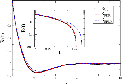
Figure 1: (Color online) Response functions measured in numerical simulations of the model with Coulomb friction (7). Parameters are $\gamma=0.05$, $\Delta=1$, $\gamma T=0.5$, $\mu=0.25$ and perturbation $h=0.1$. Inset: zoom of the discrepancy region in semi-log scale.

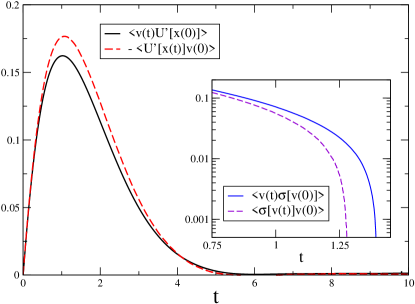
Figure 2: (Color online) Comparison among the correlation functions appearing in Eq. (16) ($\langle v(t)U^{\prime}[x(0)]\rangle$ and $\langle U^{\prime}[x(t)]v(0)\rangle$ in the main frame) measured in numerical simulations with parameters: $\gamma=0.05$, $\Delta=1$, $\gamma T=0.5$ $\mu=0.25$. Inset: Comparison among the correlation functions $\langle v(t)\sigma[v(0)]\rangle$ and $\langle\sigma[v(t)]v(0)\rangle$ in semi-log scale.

Here we are interested in the use of the FDR as a tool to point out nonequilibrium conditions. Therefore we investigate the FDR for the model introduced above in the stationary regime. We start by deriving a general expression for the response function $R(t,t^{\prime})$ of the velocity $v(t)$ to a perturbation $h(t^{\prime})$ applied at a previous time $t^{\prime}$:

$$R(t,t^{\prime})=\left.\frac{\delta\langle v(t)\rangle}{\delta h(t^{\prime})}\right|_{h=0}.$$ (10)

Since for Langevin-like systems with Gaussian noise the response can be expressed as KV94

$$R(t,t^{\prime})=\frac{1}{2\gamma T}\langle v(t)\eta(t^{\prime})\rangle,$$ (11)

substituting the expression for the noise, and considering a stationary state, where time-translational invariance holds, fixing $t^{\prime}=0$ we can write

$$R(t)=\frac{1}{2\gamma T}\Big{\{}\langle v(t)\dot{v}(0)\rangle+\langle v(t)F[v(0)]\rangle+\langle v(t)U^{\prime}[x(0)]\rangle\Big{\}}.$$ (12)

Then, exploiting the fact that $\langle v(t)\dot{v}(0)\rangle=-\langle\dot{v}(t)v(0)\rangle$, and that $\langle\eta(t)v(0)\rangle=0$ by causality, we can recast Eq. (12) in the form

$$R(t) = \frac{1}{2\gamma T}\Big{\{}\langle v(t)F[v(0)]\rangle+\langle F[v(t)]v(0)\rangle$$ (13)

$$+ \langle v(t)U^{\prime}[x(0)]\rangle+\langle U^{\prime}[x(t)]v(0)\rangle\Big{\}}.$$

This expression represents an extension to inertial cases of the result obtained in CKP94 for overdamped dynamics. Notice that in the case of a quadratic potential $U(x)=kx^{2}/2$, Eq. (13) can be further simplified, exploiting the relation $\langle x(t)v(0)\rangle=-\langle v(t)x(0)\rangle$, and one gets

$$R(t)=\frac{1}{2\gamma T}\left\{\langle v(t)F[v(0)]\rangle+\langle F[v(t)]v(0)\rangle\right\}.$$ (14)

When an equilibrium stationary state is attained, using the Onsager reciprocity relations $\langle v(t)F[v(0)]\rangle=\langle F[v(t)]v(0)\rangle$ and $\langle v(t)U^{\prime}[x(0)]\rangle=-\langle U^{\prime}[x(t)]v(0)\rangle$, one finds the EFDR

$$R_{EFDR}(t)=\frac{1}{\gamma T}\langle v(t)F[v(0)]\rangle.$$ (15)

In the presence of Coulomb friction (7), Eq. (13) takes the following expression, that we denote by $R_{FDR}$

$$R_{FDR}(t) = \frac{1}{T}\Big{\{}\langle v(t)v(0)\rangle$$ (16)

$$+ \frac{\Delta}{2\gamma}\left[\langle v(t)\sigma[v(0)]\rangle+\langle\sigma[v(t)]v(0)\rangle\right]$$

$$+ \frac{1}{2\gamma}\left[\langle v(t)U^{\prime}[x(0)]\rangle+\langle U^{\prime}[x(t)]v(0)\rangle\right]\Big{\}}.$$

As shown in Sec. II.1, in the absence of external potential an equilibrium state is attained and one obtains the EFDR with Coulomb friction

$$R_{EFDR}(t)=\frac{1}{T}\left\{\langle v(t)v(0)\rangle+\frac{\Delta}{\gamma}\langle v(t)\sigma[v(0)]\rangle\right\}.$$ (17)

In Fig. 1 we report numerical simulations of the response function $R(t)$ for the model with dry friction (7), in the presence of the ratchet potential, Eq. (9), and we compare it with the EFDR, Eq. (17), and the generalized FDR, Eq. (16): time-reversal symmetry is clearly broken in this system and nonequilibrium contributions have to be taken into account to obtain the correct expression for the response function. Numerical simulations are performed by integrating the Kramers equation with a time step $\delta t=10^{-5}$. The response is measured as the difference between the mean velocity in the presence of a small perturbation $h=0.1$ and the mean velocity for zero field, divided by $h$. The linear regime has been first checked by applying different values of perturbation. Data are averaged over about $10^{6}$ realizations. Notice that the response function shows a non-monotonous behavior, taking negative values. This is a phenomenon typical of inertial dynamics, and in our case it is very pronounced, at variance with the behavior reported in CC12 for a flashing ratchet model, where, for the chosen parameters, it is barely visible.

In Fig. 2 we also report the correlation functions appearing in Eq. (16) to explicitly show the violation of time-reversal symmetry in this case. Analogous results (not shown), with non-monotonic, oscillatory behaviors for the response functions, have been obtained using the frictional force of the model for active particles, Eq. (8).

IV Ratchet effect

In this Section we show how the presence of a spatial asymmetry coupled with nonequilibrium conditions produces a net average motion of the particle described by the model in Eq. (II), with different frictional forces. In particular, here we investigate the ratchet effect driven by Coulomb friction, recently shown in different systems gnoli ; SGP13 , in the context of Langevin equations. Notice that, at variance with the previous models of Brownian motors studied in the literature R02 ; HM03 , such as flashing ratchets, rocking ratchets, and deterministically forced ratchets, in our model there are no external forces driving the motor, and the only source of dissipation is the presence of Coulomb friction.

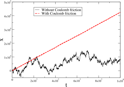
Figure 3: (Color online) Time evolution of the position $x(t)$ for the model in Eq. (II) without Coulomb friction (black continuous lines), with parameters $\gamma=0.05$, $\gamma T=0.5$, and $\mu=0.4$, and with Coulomb friction (red dashed line), with same parameters and $\Delta=1$.

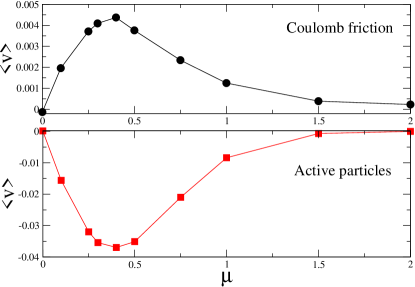
Figure 4: (Color online) Average drift for the model with Coulomb friction (7) (top panel) with parameters $\Delta=1$, $\gamma=0.05$, $\gamma T=0.5$, and for the model for active particles (8) (low panel) with parameters $\gamma_{1}=\gamma_{2}=1$, and $\gamma T=0.5$, as a function of the asymmetry parameter $\mu$ of the spatial potential, Eq. (9).

In Fig. 3 we show the time evolution of the position of the Brownian particle described by Eq. (II), in the absence (continuous black line) and in the presence of Coulomb friction (dashed red line). Only in the latter case a net ratchet effect can be clearly observed, whereas in the former case one observes large fluctuations around zero. This is due to the fact that, as discussed in Sec. II.1, if only linear friction is considered, the system attains an equilibrium stationary state and no ratchet effect can occur. On the other hand, it is interesting to study the behavior of the system upon varying the parameters entering the model. In particular, in Fig. 4 (top panel) we report the average velocity of the particle described by Eq. (II) with Coulomb friction (7), as a function of the asymmetry parameter $\mu$ of the ratchet potential, Eq. (9). In the lower panel of the same figure, we also report the results of numerical simulations of the model for active particles described by Eq. (8). As expected, for $\mu=0$, the ratchet effect vanishes in both models, because the potential is spatially symmetric in that case. By increasing the value of $\mu$ a non-monotonic behavior is observed: notice, in particular, that a peak at the same value $\mu\simeq 0.4$ is observed for both the models (see Fig. 4). This means that the maximization of the ratchet effect as a function of the shape of the potential is independent of the specific models considered. The decreasing of the ratchet effect for large values of $\mu$ is probably due to the fact that the potential develops more than one minimum. This causes an overall slowing down of the dynamics and, therefore, of the average velocity.

V Conclusions

In this article we have presented a numerical study of the Kramers equation describing the motion of a particle in an asymmetric potential and in the presence of nonlinear frictional forces, in particular the Coulomb frictional force. We have characterized the nonequilibrium behavior of the system by studying the generalized fluctuation-dissipation relation, pointing out the breaking of time-reversal symmetry when both nonlinear velocity-dependent friction forces and external potential are present. In such situations, even if no other external forces are present and the only source of fluctuations is the thermal noise of the Langevin equation, we have shown that the Coulomb friction can be a source of dissipation sufficient to drive a motor effect.

This kind of ratchet effect could be studied in experiments in nano- and micro-devices, where the presence of dry friction is still present and strongly affect the dynamical properties of the system GTVT10 ; VMUZT13 .

It would be also very useful to obtain analytical approximate expressions for the average drift of the particle in the presence of Coulomb friction. Moreover, the ratchet effect should be further characterized by studying its energetics and efficiency at maximum power, when also an external load is applied to the system.

- (1) J. L. Lebowitz and H. Spohn, J. Stat. Phys. 95, 333 (1999)
- (2) C. Maes, J. Stat. Phys. 95, 367 (1999)
- (3) A. Crisanti and F. Ritort, J. Phys. A 36, R181 (2003)
- (4) U. Marini Bettolo Marconi, A. Puglisi, L. Rondoni, and A. Vulpiani, Phys. Rep. 461, 111 (2008)
- (5) U. Seifert, Rep. Prog. Phys. 75, 126001 (2012)
- (6) M. Baiesi and C. Maes, New J. Phys. 15, 013004 (2013)
- (7) R. P. Feynman, R. B. Leighton, and M. Sands, The Feynman Lectures on Physics (Addison-Wesley, Reading, MA, 1963)
- (8) P. Reimann, Phys. Rep. 361, 57 (2002)
- (9) F. Cottone, H. Vocca, and L. Gammaitoni, Phys. Rev. Lett. 102, 080601 (2009)
- (10) T. Elston, H. Wang, and G. Oster, Nature 391, 510 (1998)
- (11) M. Schliwa and G. Woehlke, Nature 422, 759 (2003)
- (12) R. D. Astumian, Science 276, 917 (1997)
- (13) F. Jülicher, A. Ajdari, and J. Prost, Rev. Mod. Phys. 69, 1269 (1997)
- (14) P. Hänggi and F. Marchesoni, Rev. Mod. Phys. 81, 387 (2003)
- (15) J. M. R. Parrondo and B. J. De Cisneros, Appl. Phys. A 75, 179 (2002)
- (16) K. Sekimoto, Stochastic Energetics (Springer-Verlag, Berlin, 2010)
- (17) V. O. Kharchenko and I. Goychuk, Phys. Rev. E 87, 052119 (2013)
- (18) T. Schmiedl and U. Seifert, Phys. Rev. Lett. 98, 108301 (2007)
- (19) Z. C. Tu, J. Phys. A: Math. Theor. 41, 312003 (2008)
- (20) M. Esposito, R. Kawai, K. Lindenberg, and C. Van den Broeck, Phys. Rev. Lett. 105, 150603 (2010)
- (21) J. Talbot, A. Burdeau, and P. Viot, J. Stat. Mech., P03009(2011)
- (22) N. Golubeva, A. Imparato, and L. Peliti, Europhys. Lett. 97, 60005 (2012)
- (23) D. Lacoste and K. Mallick, Phys. Rev. E 80, 021923 (2009)
- (24) M. Badouals, F. Jülicher, and J. Prost, Proc. Natl. Acad. Sci. 99, 6696 (2002)
- (25) M. N. Artyomov, A. Y. Morozov, and A. B. Kolomeisky, Phys. Rev. E 77, 040901 (2008)
- (26) P.-G. de Gennes, J. Stat. Phys. 119, 953 (2005)
- (27) T. K. Caughey and J. K. Dienes, J. Appl. Phys. 32, 2476 (1961)
- (28) H. Hayakawa, Physica D 205, 48 (2005)
- (29) S. Daniel, M. K. Chaudhury, and P. G. de Gennes, Langmiur 21, 4240 (2005)
- (30) A. V. Plyukhin and A. M. Froese, Phys. Rev. E 76, 031121 (2007)
- (31) H. Touchette, E. Van der Straeten, and W. Just, J. Phys. A: Math. Theor. 43, 445002 (2010)
- (32) A. Baule, H. Touchette, and E. G. D. Cohen, Nonlinearity 24, 351 (2011)
- (33) H. Touchette, T. Prellberg, and W. Just, J. Phys. A: Math. Theor. 45, 395002 (2012)
- (34) P. S. Goohpattader and M. K. Chaudhury, Eur. Phys. J. E 35, 67 (2012)
- (35) D. Fleishman, J. Klafter, M. Porto, and M. Urbakh, Nano Lett. 7, 837 (2007)
- (36) J. Talbot, R. D. Wildman, and P. Viot, Phys. Rev. Lett. 107, 138001 (2011)
- (37) A. Baule and P. Sollich, Europhys. Lett. 97, 20001 (2012)
- (38) A. Gnoli, A. Petri, F. Dalton, G. Gradenigo, G. Pontuale, A. Sarracino, and A. Puglisi, Phys. Rev. Lett. 110, 120601 (2013)
- (39) A. Sarracino, A. Gnoli, and A. Puglisi, Phys. Rev. E 87, 040101(R) (2013)
- (40) B. Cleuren and C. Van den Broeck, Europhys. Lett. 77, 50003 (2007)
- (41) G. Costantini, A. Puglisi, and U. Marini Bettolo Marconi, J. Stat. Mech., P07004(2009)
- (42) P. Eshuis, K. van der Weele, D. Lohse, and D. van der Meer, Phys. Rev. Lett. 104, 248001 (2010)
- (43) J. Blaschke and J. Vollmer, Phys. Rev. E 87, 040201 (2013)
- (44) A. Gnoli, A. Puglisi, and H. Touchette, Europhys. Lett. 102, 14002 (2013)
- (45) A. Gnoli, A. Sarracino, A. Puglisi, and A. Petri, Phys. Rev. E 87, 052209 (2013)
- (46) F. Schweitzer, W. Ebeling, and B. Tilch, Phys. Rev. Lett. 80, 5044 (1998)
- (47) Y. L. Klimontovich, Phys.-Usp. 37, 737 (1994)
- (48) H. Risken, The Fokker-Planck equation: Methods of solution and applications (Springer- Verlag, Berlin, 1989)
- (49) A. A. Dubkov, P. Hänggi, and I. Goychuk, J. Stat. Mech., P01034(2009)
- (50) M. Polettini, Phys. Rev. E 87, 032126 (2013)
- (51) J. W. Rayleigh, The Theory of Sound (Dover, New York, 1945)
- (52) J. Farago, Physica A 331, 69 (2004)
- (53) B. Lindner, J. Stat. Phys. 130, 523 (2008)
- (54) R. Bartussek, P. Hänggi, and J. G. Kissner, Europhys. Lett. 28, 459 (1994)
- (55) F. Schweitzer, B. Tilch, and W. Ebeling, Eur. Phys. J. B 14, 157 (2000)
- (56) A. Fiasconaro, W. Ebeling, and E. Gudowska-Nowak, Eur. Phys. J. B 65, 403 (2008)
- (57) L. F. Cugliandolo, J. Kurchan, and G. Parisi, J. Phys. I France 4, 1641 (1994)
- (58) E. Lippiello, F. Corberi, and M. Zannetti, Phys. Rev. E 71, 036104 (2005)
- (59) T. Speck and U. Seifert, Europhys. Lett. 74, 391 (2006)
- (60) E. Lippiello, F. Corberi, A. Sarracino, and M. Zannetti, Phys. Rev. E 78, 041120 (2008)
- (61) M. Baiesi, E. Boksenbojm, C. Maes, and B. Wynants, J. Stat. Phys. 139, 492 (2010)
- (62) V. V. Konotop and L. Vazquez, Nonlinear Random Waves (World Scientific, Singapore, 1994)
- (63) D. Chaudhuri and A. Chaudhuri, Phys. Rev. E 85, 021102 (2012)
- (64) R. Guerra, U. Tartaglini, A. Vanossi, and E. Tosatti, Nature Materials 9, 634 (2010)
- (65) A. Vanossi, N. Manini, M. Urbakh, S. Zapperi, and E. Tosatti, Rev. Mod. Phys. 85, 529 (2013)