Stochastic Dual Coordinate Ascent
with Alternating Direction Multiplier Method

Abstract

We propose a new stochastic dual coordinate ascent technique that can be applied to a wide range of regularized learning problems. Our method is based on Alternating Direction Multiplier Method (ADMM) to deal with complex regularization functions such as structured regularizations. Although the original ADMM is a batch method, the proposed method offers a stochastic update rule where each iteration requires only one or few sample observations. Moreover, our method can naturally afford mini-batch update and it gives speed up of convergence. We show that, under mild assumptions, our method converges exponentially. The numerical experiments show that our method actually performs efficiently.

Keywords: Stochastic Dual Coordinate Ascent, Alternating Direction Multiplier Method, Exponential Convergence, Structured Sparsity.

1 Introduction

This paper proposes a new stochastic optimization method that shows exponential convergence and can be applied to wide range of regularization functions using the techniques of stochastic dual coordinate ascent with alternating direction multiplier method. Recently, it is getting more and more important to develop an efficient optimization method which can handle large amount of samples. One of the most successful approaches is a stochastic optimization approach. Indeed, a lot of stochastic methods have been proposed to deal with large amount of samples. Among them, the (online) stochastic gradient method is the most basic and successful one. This can be naturally applied to the regularized learning frame-work. Such a method is called several different names including online proximal gradient descent, forward-backward splitting and online mirror descent (Duchi and Singer, 2009). Basically, these methods are intended to process sequentially coming data. They update the parameter using one new observation and discard the observed sample. Therefore, they don’t need large memory space to store the whole observed data. The convergence rate of those methods is $O(1/\sqrt{T})$ for general settings and $O(1/T)$ for strongly convex losses, which are minimax optimal (Nemirovskii and Yudin, 1983).

On the other hand, recently it was shown that, if it is allowed to reuse the observed data several times, it is possible to develop a stochastic method with exponential convergence rate for a strongly convex objective (Le Roux et al., 2013; Shalev-Shwartz and Zhang, 2013c; Shalev-Shwartz and Zhang, 2013a). These methods are still stochastic in a sense that one sample or small mini-batch is randomly picked up to be used for each update. The main difference from the stochastic gradient method is that these methods are intended to process data with a fixed number of training samples. Stochastic Average Gradient (SAG) method (Le Roux et al., 2013) utilizes an averaged gradient to show an exponential convergence. Stochastic Dual Coordinate Ascent (SDCA) method solves the dual problem using a stochastic coordinate ascent technique (Shalev-Shwartz and Zhang, 2013c; Shalev-Shwartz and Zhang, 2013a). These methods have favorable properties of both online-stochastic approach and batch approach. That is, they show fast decrease of the objective function in the early stage of the optimization as online-stochastic approaches, and shows exponential convergence after the “burn in” time as batch approaches. However, these methods have some drawbacks. SAG needs to maintain all gradients computed on each training sample in memory which amount to dimension times sample size. SDCA method can be applied only to a simple regularization function for which the dual function is easily computed, thus it is hard to apply the method to a complex regularization function such as structured regularization.

In this paper, we propose Stochastic Dual Coordinate Ascent method for Alternating Direction Multiplier Method (SDCA-ADMM). Our method is similar to SDCA, but inherits a favorable property of ADMM. By combining SDCA and ADMM, our method can be applied to a wide range of regularized learning problems. ADMM is an effective optimization method to solve a composite optimization problem described as $\min_{x}f(x)+g(y)~{}\mathrm{s.t.}~{}Ax+By=0$ (Gabay and Mercier, 1976; Boyd et al., 2010; Qin and Goldfarb, 2012). This formulation is quite flexible and fit wide range of applications such as structured regularization, dictionary learning, convex tensor decomposition and so on (Qin and Goldfarb, 2012; Jacob et al., 2009; Tomioka et al., 2011; Rakotomamonjy, 2013). However, ADMM is a batch optimization method. Our approach transforms ADMM to a stochastic one by utilizing stochastic coordinate ascent technique. Our method, SDCA-ADMM, does not require large amount of memory because it observes only one or few samples for each iteration. SDCA-ADMM can be naturally adapted to a sub-batch situation where a block of few samples is utilized for each iteration. Moreover, it is shown that our method shows exponential convergence for risk functions with some strong convexity and smoothness property. The convergence rate is affected by the size of sub-batch. If the samples are not strongly correlated, sub-batch gives a better convergence rate than one-sample update.

2 Structured Regularization and its Dual Formulation

In this section, we give the problem formulation of structured regularization and its dual formulation. The standard regularized risk minimization is described as follows:

$$\min_{w\in\mathbb{R}^{p}}\frac{1}{n}\sum_{i=1}^{n}f_{i}(z_{i}^{\top}w)+\tilde{\psi}(w),$$ (1)

where $z_{1},z_{2},\dots,z_{n}$ are vectors in $\mathbb{R}^{p}$, $w$ is the weight vector that we want to learn, $f_{i}$ is a loss function for the $i$-th sample, and $\tilde{\psi}$ is the regularization function which is used to avoid over-fitting. For example, the loss function $f_{i}$ can be taken as a classification surrogate loss $f_{i}(z_{i}^{\top}w)=\ell(y_{i},z_{i}^{\top}w)$ where $y_{i}$ is the training label of the $i$-th sample. With regard to $\tilde{\psi}$, we are interested in a sparsity inducing regularization, e.g., $\ell_{1}$-regularization, group lasso regularization, trace-norm regularization, and so on. Our motivation in this paper is to deal with a “complex” regularization $\tilde{\psi}$ where it is not easy to directly minimize the regularization function (more precisely the proximal operation determined by $\tilde{\psi}$ is not easily computed, see Eq. (5)). This kind of regularization appears in, for example, structured sparsity such as overlapped group lasso and graph regularization (Jacob et al., 2009; Signoretto et al., 2010). In many cases, such a “complex” regularization function can be decomposed into a “simple” regularization $\psi$ and a linear transformation $B$, that is, $\tilde{\psi}(w)=\psi(B^{\top}w)$ where $B\in\mathbb{R}^{p\times d}$ . Using this formulation, the optimization problem (Eq. (1)) is equivalent to

$$\min_{w\in\mathbb{R}^{p}}\frac{1}{n}\sum_{i=1}^{n}f_{i}(z_{i}^{\top}w)+\psi(B^{\top}w).$$ (2)

The purpose of this paper is to give an efficient stochastic optimization method to solve this problem (2). For this purpose, we employ the dual formulation. Using the Fenchel’s duality theorem, we have the following dual formulation.

Lemma 1.

$$\min_{w\in\mathbb{R}^{p}}\frac{1}{n}\sum_{i=1}^{n}f_{i}(z_{i}^{\top}w)+\psi(B^{\top}w)$$

$$= -\!\!\min_{x\in\mathbb{R}^{n},y\in\mathbb{R}^{d}}\left\{\frac{1}{n}\sum_{i=1}^{n}f_{i}^{*}(x_{i})+\psi^{*}\big{(}\frac{y}{n}\big{)}\mid Zx+By=0\right\},$$ (3)

where $f_{i}^{*}$ and $\psi^{*}$ are the convex conjugates of $f_{i}$ and $\psi$ respectively (Rockafellar, 1970), and $Z=[z_{1},z_{2},\dots,z_{n}]\in\mathbb{R}^{p\times n}$. Moreover $w^{*}$, $x^{*}$ and $y^{*}$ are optimal solutions of both sides if and only if

$$z_{i}^{\top}w^{*}\in\nabla f_{i}^{*}(x_{i}^{*}),~{}\frac{1}{n}y^{*}\in\nabla\psi(u)|_{u=B^{\top}w^{*}},$$

$$Zx^{*}+By^{*}=0.$$

Proof.

By Fenchel’s duality theorem (Corollary 31.2.1 of Rockafellar (1970)), we have that

$$\min_{w\in\mathbb{R}^{p}}\frac{1}{n}\sum_{i=1}^{n}f_{i}(z_{i}^{\top}w)+\tilde{\psi}(w)=-\min_{x\in\mathbb{R}^{n}}\left\{\frac{1}{n}\sum_{i=1}^{n}f_{i}^{*}(x_{i})+\tilde{\psi}^{*}(-Zx/n)\right\}.$$ (4)

Moreover $x^{*},w^{*}$ are optimal of each side if and only if $z_{i}^{\top}w^{*}\in\nabla f_{i}^{*}(x^{*}_{i})$ and $-Zx^{*}/n\in\nabla\tilde{\psi}(w^{*})=B\nabla\psi(u^{*})|_{u=B^{\top}w^{*}}$ (Corollary 31.3 of Rockafellar (1970)). Now, Theorem 16.3 of Rockafellar (1970) gives that

$$\tilde{\psi}^{*}(u)=(\psi\circ B^{\top})^{*}(u)=\inf\{\psi^{*}(y)\mid By=u\}.$$

Thus $\tilde{\psi}^{*}(-Zx/n)=\inf\{\psi^{*}(y/n)\mid By=-Zx\}$, and substituting this into the RHS of Eq. (4) we obtain Eq. (3). Now, $y^{*}$ satisfying $Zx^{*}+By^{*}=0$ is the optimal value if and only if $\psi^{*}(y^{*}/n)=\tilde{\psi}^{*}(-Zx^{*}/n)$ for the optimal $x^{*}$. Thus, if $(w^{*},x^{*},y^{*})$ is optimal, then we have $-Zx^{*}/n\in\nabla\tilde{\psi}(w^{*})$ and thus $\psi^{*}(y^{*}/n)=\tilde{\psi}^{*}(-Zx^{*}/n)=\langle w^{*},-Zx^{*}/n\rangle-\tilde{\psi}(w^{*})=\langle B^{\top}w^{*},y^{*}/n\rangle-\psi(B^{\top}w^{*})$ which implies $y^{*}/n\in\nabla\psi(u)|_{u=B^{\top}w^{*}}$. Contrary, if $y^{*}/n\in\nabla\psi(u)|_{u=B^{\top}w^{*}}$, then it is obvious that $-Zx^{*}/n\in\nabla\tilde{\psi}(w^{*})$ because $Zx^{*}+By^{*}=0$. Therefore, we obtain the optimality conditions.

∎

The dual problem is a composite objective function optimization with a linear constraint $Zx+By=0$. In the next section, we give an efficient stochastic method to solve this dual problem. A nice property of the dual formulation is that, in many machine learning applications, the dual loss function $f_{i}^{*}$ becomes strongly convex. For example, for the logistic loss $f_{i}(x)=\log(1+\exp(-y_{i}x))$, the dual function is $f_{i}^{*}(-u)=y_{i}u\log(y_{i}u)+(1-y_{i}u)\log(1-y_{i}u)~{}(y_{i}u\in[0,1])$ and its modulus of strong convexity is much better than the primal one. More importantly, each sample $(z_{i},y_{i})$ directly affects only each coordinate $x_{i}$ of dual variable. In other words, if $x_{i}$ is fixed the $i$-th sample $(z_{i},y_{i})$ has no influence to the objective value. This enables us to utilize the stochastic coordinate ascent technique in the dual problem because update of single coordinate $x_{i}$ requires only the information of the $i$-th sample $(z_{i},y_{i})$.

Finally, we give the precise notion of the “complex” and “simple” regularizations. This notion is defined by the computational complexity of proximal operation corresponding to the regularization function (Rockafellar, 1970). The proximal operation corresponding to a convex function $\psi$ is defined by

$$\mathrm{prox}(q|\psi):=\mathop{\arg\min}_{u}\left\{\frac{1}{2}\|q-u\|^{2}+\psi(u)\right\}.$$ (5)

For example, the proximal operation corresponding to $\ell_{1}$-regularization $\psi(w)=\|w\|_{\ell_{1}}$ is easily computed as $\mathrm{prox}(q|\psi)=(\mathrm{sign}(w_{i})\max\{|w_{i}|-1,0\})_{i}$ which is the so-called soft-thresholding operation. More generally, the proximal operation for group lasso regularization with non-overlapped groups can also be analytically computed. On the other hand, for overlapped group regularization, the proximal operation is no longer analytically obtained. However, by choosing $B$ appropriately, we can split the overlap and obtain $\psi$ for which the proximal operation is easily computed (see Section 6 for concrete examples).

3 Proposed Method: Stochastic Dual Coordinate Ascent with ADMM

In this section, we present our proposal, stochastic dual coordinate ascent type ADMM. For a positive semidefinite matrix $S$, we denote by $\|x\|_{S}:=\sqrt{x^{\top}Sx}$. $Z_{i}$ denotes the $i$-th column of $Z$, which is $z_{i}$, and $Z_{\backslash i}$ is a matrix obtained by subtracting $i$-th column from $Z$. Similarly, for a vector $x$, $x_{\backslash i}$ is a vector obtained by subtracting $i$-th component from $x$.

3.1 One Sample Update of SDCA for ADMM

The basic update rule of our proposed method in the $t$-th step is given as follows: Each update step, choose $i\in\{1,\dots,n\}$ uniformly at random, and update as

$$y^{(t)}\!\!\leftarrow \mathop{\arg\min}_{y}\Big{\{}n\psi^{*}(y/n)-\langle w^{(t-1)}\!\!,Zx^{(t-1)}\!+\!By\rangle+\frac{\rho}{2}\|Zx^{(t-1)}+By\|^{2}+\frac{1}{2}\|y-y^{(t-1)}\|_{Q}^{2}\Big{\}},$$ (6a)

$$x^{(t)}_{i}\!\!\leftarrow \mathop{\arg\min}_{x_{i}}\Big{\{}f_{i}^{*}(x_{i})-\langle w^{(t-1)},Z_{i}x_{i}+By^{(t)}\rangle+\frac{\rho}{2}\|Z_{i}x_{i}+Z_{\backslash i}x^{(t-1)}_{\backslash i}+By^{(t)}\|^{2}$$

$$~{}~{}~{}~{}~{}~{}~{}~{}~{}~{}~{}~{}~{}~{}~{}~{}+\frac{1}{2}\|x_{i}-x^{(t-1)}_{i}\|_{G_{ii}}^{2}\Big{\}},$$ (6b)

$$w^{(t)}\!\!\leftarrow w^{(t-1)}-\gamma\rho\{n(Zx^{(t)}+By^{(t)})-(n-1)(Zx^{(t-1)}+By^{(t-1)})\},$$ (6c)

where $w^{(t)}\in\mathbb{R}^{p}$ is the primal variable at the $t$-th step, $Q$ and $G$ are arbitrary positive semidefinite matrices, and $\gamma,\rho>0$ are parameters we give beforehand.

The optimization procedure looks a bit complicated, To simplify the procedure, we set $Q$ as

$$Q=\rho(\eta_{B}\mathrm{I}_{d}-B^{\top}B)$$ (7)

where $\eta_{B}$ are chosen so that $\eta_{B}\mathrm{I}_{d}\succ B^{\top}B$. Then, by carrying out simple calculations and denoting $\eta_{Z,i}=G_{ii}/\rho+\|z_{i}\|^{2}$, the update rule of $x^{(t)}$ and $y^{(t)}$ is rewritten as

$$y^{(t)}\!\!\leftarrow\mathrm{prox} \Big{(}y^{(t-1)}+\frac{B^{\top}}{\rho\eta_{B}}\{w^{(t-1)}-\rho(Zx^{(t-1)}+By^{(t-1)})\}~{}\Big{|}~{}\frac{n\psi^{*}(\cdot/n)}{\rho\eta_{B}}\Big{)},$$ (8a)

$$x^{(t)}_{i}\leftarrow\mathrm{prox} \Big{(}x^{(t-1)}_{i}+\frac{Z_{i}^{\top}}{\rho\eta_{Z,i}}\{w^{(t-1)}-\rho(Zx^{(t-1)}+By^{(t)})\}~{}\Big{|}~{}\frac{f_{i}^{*}}{\rho\eta_{Z,i}}\Big{)}.$$ (8b)

Note that the update (8b) of $x^{(t)}$ is just a one dimensional optimization, thus it is quite easily computed. Moreover, for some loss functions such as the smoothed hinge loss used in Section 6, we have an analytic form of the update.

The update rule (8a) of $y^{(t)}$ can be rewritten by the proximal operation corresponding to the primal function $\psi$ while the rule (8a) is given by that corresponding to the dual function $\psi^{*}$. Indeed, there is a clear relation between primal and dual (Theorem 31.5 of Rockafellar (1970)):

$$\mathrm{prox}(q|\psi)+\mathrm{prox}(q|\psi^{*})=q.$$

Using this, for $q^{(t)}=y^{(t-1)}+\frac{B^{\top}}{\rho\eta_{B}}\{w^{(t-1)}-\rho(Zx^{(t-1)}+By^{(t-1)})\}$, we have that

$$y^{(t)}\leftarrow q^{(t)}-\mathrm{prox}(q^{(t)}|n\psi(\rho\eta_{B}~{}\cdot~{})/(\rho\eta_{B})),$$ (9)

because $(cf(\cdot))^{*}(y)=cf^{*}(y/c)$ for a convex function $f$ and $c>0$. This is efficiently computed because we assumed the proximal operation corresponding to $\psi$ can be efficiently computed.

During the update, we need $Zx^{(t-1)}$ which seems to require $O(n)$ computation at the first glance. However, it can be incrementally updated as $Zx^{(t)}=Zx^{(t-1)}+Z_{i}(x^{(t)}_{i}-x^{(t-1)}_{i})$. Thus we don’t need to road all the samples to compute $Zx^{(t-1)}$ at each iteration.

In the above, the update rule of our algorithm is based on one sample observation. Next, we give a mini-batch extension of the algorithm where more than one samples could be used for each iteration.

3.2 Mini-Batch Extension

Here, we generalize our method to mini-batch situation where, at each iteration, we observe a small number of samples $\{(x_{i_{1}},y_{i_{1}}),\dots,(x_{i_{k}},y_{i_{k}})\}$ instead of one sample observation. At each iteration, we randomly choose an index set $I\subseteq\{1,\dots,n\}$ so that each index $i$ is included in $I$ with probability $1/K$; $P(i\in I)=1/K$ for all $i=1,\dots,n$. To do so, we suggest the following procedure. We split the index set $\{1,\dots,n\}$ into $K$ groups $(I_{1},I_{2},\dots,I_{K})$ beforehand, and then pick up uniformly $k\in\{1,\dots,K\}$ and set $I=I_{k}$ for each iteration. Each sub-batch $I_{k}$ can have different cardinality from others, but the probability $P(i\in I)$ should be uniform for all $i=1,\dots,n$. The update rule using sub-batch is given as follows: Update $y^{(t)}$ as before (6a), and update $x^{(t)}$ and $w^{(t)}$ by

$$x^{(t)}_{I}\leftarrow\mathop{\arg\min}_{x_{I}}\Big{\{}\sum_{i\in I}f_{i}^{*}(x_{i})-\langle w^{(t-1)},Z_{I}x_{I}+By^{(t)}\rangle+\frac{\rho}{2}\|Z_{I}x_{I}+Z_{\backslash I}x^{(t-1)}_{\backslash I}+By^{(t)}\|^{2}$$

$$~{}~{}~{}~{}~{}~{}~{}~{}~{}~{}~{}~{}~{}~{}~{}~{}~{}~{}~{}~{}~{}~{}~{}~{}~{}~{}~{}~{}+\frac{1}{2}\|x_{I}-x^{(t-1)}_{I}\|_{G_{I,I}}^{2}\Big{\}},$$ (10a)

$$w^{(t)}\leftarrow w^{(t-1)}-\gamma\rho\{n(Zx^{(t)}+By^{(t)})-(n-n/K)(Zx^{(t-1)}+By^{(t-1)})\}.$$ (10b)

Using $Q$ given in Eq. (7), the update rule of $y^{(t)}$ can be replaced by Eq. (9) as in one-sample update situation. The update rule of $x^{(t)}$ can also be simplified by choosing $G$ appropriately. Because sub-batches have no overlap between each other, we can construct a positive semi-definite matrix $G$ such that the block-diagonal element $G_{I,I}$ has the form

$$G_{I,I}=\rho(\eta_{Z,I}-Z_{I}^{\top}Z_{I})$$ (11)

where $\eta_{Z,I}$ is a positive real satisfying $\eta_{Z,I}\geq\|Z_{I}^{\top}Z_{I}\|$. The reason why we split the index sets into $K$ sets is to construct this kind of $G$ which “diagonalizes” the quadratic function in (10a). The choice of $I$ and $G$ could be replaced with another one for which we could compute the update efficiently, as long as $P(i\in I)$ is uniform for all $i=1,\dots,n$. Using $G$ given in (11), the update rule (10a) of $x^{(t)}$ is rewritten as

$$x^{(t)}_{I}\leftarrow\mathrm{prox} \Big{(}x^{(t-1)}_{I}+\frac{Z_{I}^{\top}}{\rho\eta_{Z,I}}\{w^{(t-1)}-\rho(Zx^{(t-1)}+By^{(t)})\}~{}\Big{|}~{}\frac{\sum_{i\in I}f_{i}^{*}}{\rho\eta_{Z,I}}\Big{)},$$ (12)

where $x_{I}$ is a vector consisting of components with indexes $i\in I$, $x_{I}=(x_{i})_{i\in I}$, and $Z_{I}$ is a sub-matrix of $Z$ consisting of columns with indexes $i\in I$, $Z_{I}=[Z_{i_{1}},\dots,Z_{i_{|I|}}]$. Note that, since $\sum_{i\in I}f_{i}^{*}(x_{i})$ is sum of single variable convex functions $f_{i}^{*}(x_{i})$, the proximal operation in Eq. (12) can be split into the proximal operation with respect to each single variable $x_{i}$. This is advantageous for not only the simpleness of the computation but also parallel computation. That is, for $p_{I}=x^{(t-1)}_{I}+\frac{Z_{I}^{\top}}{\rho\eta_{Z,I}}\{w^{(t-1)}-\rho(Zx^{(t-1)}+By^{(t)})\}$, the update rule (12) is reduced to $x^{(t)}_{i}\leftarrow\mathrm{prox}(p_{i}|\frac{f_{i}^{*}}{\rho\eta_{Z,I}})$ for each $i\in I$, which is easily parallelizable. In summary, our proposed algorithm is given in Algorithm 1.

Algorithm 1 SDCA-ADMM

  Input: $\rho,\eta>0$

  Initialize $x_{0}=\boldsymbol{0}$, $y_{0}=\boldsymbol{0}$, $w_{0}=\boldsymbol{0}$ and $\{I_{1},\dots,I_{K}\}$.

  for $t=1$ to $T$  do

     Choose $k\in\{1,\dots,K\}$ uniformly at random, set $I=I_{k}$, and observe the training samples $\{(x_{i},y_{i})\}_{i\in I}$.

     Set $q^{(t)}\!\!=\!y^{(t-1)}\!+\frac{B^{\top}}{\rho\eta_{B}}\{w^{(t-1)}\!-\!\rho(Zx^{(t-1)}\!+\!By^{(t-1)})\}$.

     Update $y^{(t)}\leftarrow q^{(t)}-\mathrm{prox}(q^{(t)}|n\psi(\rho\eta_{B}~{}\cdot~{})/(\rho\eta_{B}))$

     Update $x^{(t)}_{I}\leftarrow\mathrm{prox}\Big{(}x^{(t-1)}_{I}+\frac{Z_{I}^{\top}}{\rho\eta_{Z,I}}\{w^{(t-1)}-\rho(Zx^{(t-1)}+By^{(t)})\}~{}\Big{|}~{}\frac{\sum_{i\in I}f_{i}^{*}}{\rho\eta_{Z,I}}\Big{)}.$

     Update $w^{(t)}\leftarrow w^{(t-1)}-\gamma\rho\{n(Zx^{(t)}+By^{(t)})-(n-n/K)(Zx^{(t-1)}+By^{(t-1)})\}$.

  end for

  Output: $w^{(T)}$.

Finally, we would like to highlight the connection between our method and the original batch ADMM (Hestenes, 1969; Powell, 1969; Rockafellar, 1976). The batch ADMM utilizes the following update rule

$$y^{(t)}\leftarrow \mathop{\arg\min}_{y}\Big{\{}n\psi^{*}\left(\frac{y}{n}\right)-\langle w^{(t-1)},Zx^{(t-1)}+By\rangle+\frac{\rho}{2}\|Zx^{(t-1)}+By\|^{2}\Big{\}},$$ (13a)

$$x^{(t)}\leftarrow \mathop{\arg\min}_{x}\big{\{}{\textstyle\sum_{i=1}^{n}f_{i}^{*}(x_{i})}-\langle w^{(t-1)},Zx+By^{(t)}\rangle+\frac{\rho}{2}\|Zx+By^{(t)}\|^{2}\big{\}},$$ (13b)

$$w^{(t)}\leftarrow w^{(t-1)}-\gamma\rho(Zx^{(t)}+By^{(t)}).$$ (13c)

One can see that the update rule of our algorithm is reduced to that of the batch ADMM (13) if we set $K=1$ except the term related to $G$ and $Q$ (the terms $\frac{1}{2}\|\cdot\|_{Q}^{2}$ and $\frac{1}{2}\|\cdot\|_{G_{I,I}}^{2}$). These terms related to $G$ and $Q$ are used also in batch situation to eliminate cross terms in $BB^{\top}$ and $ZZ^{\top}$. This technique is called linearization. The linearization technique makes the update rule simple and parallelizable, and in some situations makes it possible to obtain an analytic form of the update.

4 Linear Convergence of SDCA-ADMM

In this section, the convergence rate of our proposed algorithm is given. Indeed, the convergence rate is exponential (R-linear). To show the convergence rate, we assume some conditions. First, we assume that there exits an unique optimal solution $w^{*}$ and $B^{\top}$ is injective (on the other hand, $B$ is not necessarily injective). Moreover, we assume the uniqueness of the dual solution $x^{*}$, but don’t assume the uniqueness of $y^{*}$. We denote by the set of dual optimum of $y$ as $\mathcal{Y}^{*}$ and assume that $\mathcal{Y}^{*}$ is compact. Then, by Lemma 1, we have that

$$z_{i}^{\top}w^{*}\in\nabla f_{i}^{*}(x^{*}_{i}),~{}~{}y^{*}/n\in\nabla\psi(u)|_{u=B^{\top}w^{*}}.$$ (14)

By the convex duality arguments, this implies that $x^{*}_{i}\in\nabla f_{i}(u)|_{u=z_{i}^{\top}w^{*}},~{}~{}B^{\top}w^{*}\in\nabla\psi^{*}(u)|_{u=y^{*}/n}$.

Moreover, we suppose that each (dual) loss function $f_{i}$ is locally $v$-strongly convex and $\psi$, $h$-smooth around the optimal solution and $\psi^{*}$ is also locally strongly convex in a weak sense as follows.

Assumption 1.

There exits $v>0$ such that, $\forall x_{i}\in\mathbb{R}$,

$$f_{i}^{*}(x_{i})-f_{i}^{*}(x_{i}^{*})\geq\langle\nabla f_{i}^{*}(x_{i}^{*}),x_{i}-x_{i}^{*}\rangle+\frac{v\|x_{i}-x_{i}^{*}\|^{2}}{2}.$$

There exit $h>0$ and $v_{\psi}>0$ such that, for all $y$, there exists $\widehat{y}^{*}\in\mathcal{Y}^{*}$ such that

$$\psi^{*}(y/n)-\psi^{*}(\widehat{y}^{*}/n) \geq\langle B^{\top}w^{*},y/n-\widehat{y}^{*}/n\rangle+\frac{v_{\psi}}{2}\|P_{\mathrm{Ker}(B)}(y/n-\widehat{y}^{*}/n)\|^{2},$$ (15)

and for all $y^{*}\in\mathcal{Y}^{*}$ we have

$$\psi(u)-\psi(B^{\top}w^{*}) \geq\langle y^{*}/n,u-B^{\top}w^{*}\rangle+\frac{h}{2}\|u-B^{\top}w^{*}\|^{2},$$ (16)

where $P_{\mathrm{Ker}(B)}$ is the projection matrix to the kernel of $B$.

Note that these conditions should be satisfied only around the optimal solutions $(x^{*},y^{*})$ and $w^{*}$. It does not need to hold for every point, thus is much weaker than the ordinal strong convexity. Moreover, the inequalities need to be satisfied only for the solution sequence $(w^{(t)},x^{(t)},y^{(t)})$ of our algorithm. The condition (15) is satisfied, for example, by $\ell_{1}$-regularization because the dual of $\ell_{1}$-regularization is an indicator function with a compact support and, outside the optimal solution set $\mathcal{Y}^{*}$, the indicator function is lower bounded by a quadratic function. In addition, the quadratic term in the right hand side of this condition (15) is restricted on $\mathrm{Ker}(B)$. This makes it possible to include several types of regularization functions. Indeed, if $B=\mathrm{I}_{p}$, this condition is always satisfied. The assumption (16) is the strongest assumption. This is satisfied for elastic-net regularization. If one wants to obtain a solution for non-strongly convex regularization such as $\ell_{1}$-regularization, just adding a small square term, we obtain an approximated solution which is sufficiently close to the true one within a precision.

Define the primal and dual objectives as

$$\textstyle F_{P}(w):= \frac{1}{n}\sum_{i=1}^{n}f_{i}(z_{i}^{\top}w)+\psi(B^{\top}w),$$

$$\textstyle F_{D}(x,y):= \frac{1}{n}\sum_{i=1}^{n}f_{i}^{*}(x_{i})+\psi^{*}(\textstyle\frac{y}{n})-\langle w^{*},Z\frac{x}{n}-B\frac{y}{n}\rangle.$$

Note that, by Eq. (14), $F_{P}(w)-F_{P}(w^{*})$ and $F_{D}(x,y)-F_{D}(x^{*},y^{*})$ are always non-negative. Define the block diagonal matrix $H$ as $H_{I,I}=\rho Z_{I}^{\top}Z_{I}+G_{I,I}$ for all $I\in\{I_{1},\dots,I_{K}\}$ and $H_{i,j}=0$ for $(i,j)\notin I_{k}\times I_{k}~{}(\forall k)$. Let $\|y-\mathcal{Y}^{*}\|_{Q}:=\min\{\|y-y^{*}\|_{Q}\mid y^{*}\in\mathcal{Y}^{*}\}$. We define $R_{D}(x,y,w)$ as

$$R_{D}(x,y,w):= F_{D}(x,y)-F_{D}(x^{*},y^{*})+\frac{1}{2n\gamma\rho}\|w-w^{*}\|^{2}$$

$$+\frac{\rho(1-\gamma)}{2n}\|Zx+By\|^{2}+\frac{1}{2n}\|x-x^{*}\|^{2}_{v\mathrm{I}_{p}+H}+\frac{1}{2n^{2}}\|y-\mathcal{Y}^{*}\|_{Q}^{2}.$$

For a symmetric matrix $S$, we define $\sigma_{\mathrm{max}}(S)$ and $\sigma_{\mathrm{min}}(S)$ as the maximum and minimum singular value respectively.

Theorem 2.

Suppose that $\gamma=\frac{1}{4n}$, $\eta_{Z,I}>(1+2\gamma n(1-1/K))\sigma_{\max}(Z_{I}^{\top}Z_{I})$ for all $I\in\{I_{1},\dots,I_{K}\}$ and $B^{\top}$ is injective. Then, under Assumption 1, the dual objective function converges R-linearly: We have that, for $C_{1}=R_{D}(x^{(0)},y^{(0)},w^{(0)})$,

$$\mathrm{E}[R_{D}(x^{(T)},y^{(T)},w^{(T)})]\leq\left(1-\frac{\mu}{K}\right)^{T}C_{1},$$

where

$$\mu=\min\bigg{\{}\frac{v}{4(v+\sigma_{\mathrm{max}}(H))},\frac{h\rho\sigma_{\min}(B^{\top}B)}{2\max\{1/n,4h\rho,4h\sigma_{\max(Q)}\}},\frac{v_{\psi}}{4\sigma_{\max}(Q)},\frac{nv\sigma_{\min}(BB^{\top})}{4\sigma_{\max(Q)}(\rho\sigma_{\max}(Z^{\top}Z)+4v)}\bigg{\}}.$$

In particular, we have that

$$\mathrm{E}[\|w^{(T)}-w^{*}\|^{2}]\leq\frac{n\rho}{2}\left(1-\frac{\mu}{K}\right)^{T}C_{1}.$$

If we further assume $\psi(B^{\top}w)\leq\psi(B^{\top}w^{*})+\langle y^{*}/n,B^{\top}(w-w^{*})\rangle+l_{1}\|w-w^{*}\|+l_{2}\|w-w^{*}\|^{2}$ ($\forall w$), then this implies that

$$\mathrm{E}[F_{P}(w^{(T)})-F_{P}(w^{*})]$$

$$\leq\left(\frac{\sigma_{\max}(Z^{\top}Z/n)}{2v}+l_{2}\right)\frac{n\rho}{2}\left(1-\frac{\mu}{K}\right)^{T}C_{1}+l_{1}\sqrt{\frac{n\rho}{2}\left(1-\frac{\mu}{K}\right)^{T}C_{1}}.$$

The proof is deferred to the appendix. This theorem shows that the primal and dual objective values converge R-linearly. Moreover, the primal variable $w$ also converges R-linearly to the optimal value. The number $K$ of sub-batches controls the convergence rate. If all samples are nearly orthogonal to each other, $\sigma_{\max}(H)$ is bounded by a constant for all $K$, and thus convergence rate gets faster and faster as $K$ decreases (the size of each sub-batch grows up). On the other hand, if samples are strongly correlated to each other, $\sigma_{\max}(H)$ grows linearly against $1/K$ and then the convergence rate is not improved by decreasing $K$. As for batch settings, the linear convergence of batch ADMM has been shown by (Deng and Yin, 2012). However, their proof can not be directly applied to our stochastic setting. Our proof requires a technique specialized to stochastic coordinate ascent technique. We would like to point out that the exponential convergence is not guaranteed if the choice of index set $I$ at each update is cyclic. Thus the index $I$ should be randomly chosen. This is reported also in the paper (Shalev-Shwartz and Zhang, 2013a).

The statement can be described in terms of the number of iterations required to achieve a precision $\epsilon$, i.e. smallest $T$ satisfying $\mathrm{E}[F_{P}(w^{(T)})-F_{P}(w^{*})]\leq\epsilon$:

$$T\leq C^{\prime}K\max\Bigg{\{} \frac{v+\sigma_{\mathrm{max}}(H)}{v},\frac{\max\{1/(nh),\rho,\sigma_{\max(Q)}\}}{\rho\sigma_{\min}(B^{\top}B)},$$

$$\frac{\sigma_{\max}(Q)}{v_{\psi}},\frac{\sigma_{\max}(Q)(\rho\sigma_{\max}(Z^{\top}Z)+4v)}{nv\sigma_{\min}(BB^{\top})}\Bigg{\}}\log\left(\frac{nC^{\prime\prime}}{\epsilon}\right),$$

where $C^{\prime}$ and $C^{\prime\prime}$ are an absolute constant. This says that dependency of $\epsilon$ is log-order. An interesting point is that the influence of $h$, the modulus of local strong convexity of $\psi$. Usually the regularization function is made weaker as the number of samples increases. In that situation, $h$ decreases as $n$ goes up. However, even if we set $h=1/n$, we still have $T=O(K\log(n/\epsilon))$ instead of $O(nK\log(n/\epsilon))$. Thus, the convergence rate is hardly affected by the setting of $h$. This point is same as the ordinary SDCA algorithm (Shalev-Shwartz and Zhang, 2013a).

5 Related Works

In this section, we present some related works and discuss differences from our method.

The most related work is a recent study by (Shalev-Shwartz and Zhang, 2013c) in which Stochastic Dual Coordinate Ascent (SDCA) method for a regularized risk minimization is proposed. Their method also deals with the dual problem (3) with $B=\mathrm{I}_{p}$ in our setting, and apply a stochastic coordinate ascent technique. This method converges linearly. At each iteration, the method solves the following one-dimensional optimization problem,

$$\Delta x^{(t)}_{i}\!\leftarrow\mathop{\arg\min}_{\Delta x_{i}\in\mathbb{R}} ~{}f_{i}^{*}(\Delta x_{i}+x^{(t-1)}_{i})+z_{i}^{\top}w^{(t-1)}\Delta x_{i}+\frac{1}{2n}\|z_{i}\Delta x_{i}\|^{2},$$

and updates $x^{(t)}_{i}\leftarrow\Delta x^{(t)}_{i}+x^{(t-1)}_{i}$ and $w^{(t)}\leftarrow\nabla\tilde{\psi}^{*}(-Ax^{(t)})$. The most important difference from our method is the computation of $\nabla\psi^{*}$. In a “simple” regularization function, it is often easy to compute the (sub-)gradient of $\tilde{\psi}^{*}$. However, in a “complex” regularization such as structured regularization, the computation is not efficiently carried out. To overcome this difficulty, our method utilizes a linear transformed one $\psi(B\cdot)=\tilde{\psi}(\cdot)$, and split the optimization with respect to $f_{i}^{*}$ and $\psi^{*}$ by applying ADMM technique. Thus, our method is applicable to much more general regularization functions. Recently, a mini-batch extension of SDCA is a hot topic (Takáč et al., 2013; Shalev-Shwartz and Zhang, 2013b). Our approach realizes the mini-batch extension using the linearlization technique in ADMM which is naturally derived in the frame-work of ADMM. Although the proof technique is quite different, the convergence analysis of normal mini-batch SDCA given by (Shalev-Shwartz and Zhang, 2013b) is parallel to our theorem.

The second method related to ours is Stochastic Average Gradient (SAG) method (Le Roux et al., 2013). The method is a modification of stochastic gradient descent method, but utilizes an averaged gradient. A good point of their method is that we only need to deal with the primal problem. Thus the computation is easy, and we don’t need to look at the convex conjugate function. Moreover, their method also converges linearly. However, the biggest drawback is that, to compute the averaged gradient, all gradients of loss functions computed at each sample should be stored in memory. The memory size is usually $O(p\times n)$ which is hard to be stored for big data situation. On the other hand, our method is free from such a memory problem. Indeed, our method requires only $O(p+n)$-size memory.

The third method is online version of ADMM. Recently some online variants of ADMM have been proposed by (Wang and Banerjee, 2012; Suzuki, 2013; Ouyang et al., 2013). These methods are effective for complex regularizations as discussed in this paper. Thus they are applicable to wide range of situations. However, those methods are basically online methods, thus they discard the samples once observed. They are not adapted to a situation where the training samples are observed several times. Therefore, the convergence rate is $O(1/\sqrt{T})$ in general and $O(\log(T)/T)$ for a strongly convex loss (possibly $O(1/T)$ with some modification). On the other hand, our method converges linearly.

6 Numerical Experiments

In this section, we give numerical experiments on artificial and real data to demonstrate the effectiveness of our proposed algorithm. We compare our SDCA-ADMM with the existing stochastic optimization methods such as Regularized Dual Averaging (RDA) (Duchi and Singer, 2009; Xiao, 2009), Online ADMM (OL-ADMM) (Wang and Banerjee, 2012), Online Proximal Gradient descent ADMM (OPG-ADMM) (Ouyang et al., 2013; Suzuki, 2013) and RDA-ADMM (Suzuki, 2013). We also compared our method with batch ADMM (Batch-ADMM) in the artificial data sets. We used sub-batch with size 50 for all the methods including ours ($|I_{k}|=50~{}(\forall k)$, but $|I_{K}|$ could be less than 50). We employed the parameter settings $\gamma=1/n$ and $\rho=0.1$. As for $\eta_{Z,I}$ and $\eta_{B}$, we used $\eta_{Z,I}=1.1\sigma_{\max}(Z_{I}^{\top}Z_{I})$ and $\eta_{B}=\sigma_{\max}(BB^{\top})+1$. All of the experiments are classification problems with structured sparsity. We employed the smoothed hinge loss:

$$\textstyle f_{i}(u)=\begin{cases}0,&(y_{i}u\geq 1),\\ \frac{1}{2}-y_{i}u,&(y_{i}u<0),\\ \frac{1}{2}(1-y_{i}u)^{2},&(\text{otherwise}).\end{cases}$$

Then the proximal operation with respect to the dual function of the smoothed hinge loss is analytically given by

$$\textstyle\mathrm{prox}(u|f_{i}^{*}/C)=\begin{cases}\frac{Cu-y_{i}}{1+C}&(-1\leq\frac{Cuy_{i}-1}{1+C}\leq 0),\\ -y_{i}&(-1>\frac{Cuy_{i}-1}{1+C}),\\ 0&(\text{otherwise}).\end{cases}$$

6.1 Artificial Data

Here we execute numerical experiments on artificial data sets. The problem is a classification problem with overlapped group regularization as performed in (Suzuki, 2013). We generated $n$ input feature vectors $\{z_{i}\}_{i=1}^{n}$ with dimension $d=32\times 32=1024$ where each feature is generated from i.i.d. standard normal distribution. Then the true weight vector $w_{0}$ is generated as follows: First we generate a random matrix which has non-zero elements on its first column (distributed from i.i.d. standard normal) and zeros on other columns, and vectorize the matrix to obtain $w_{0}$. The training label $y_{i}$ is given by $y_{i}=\mathrm{sign}(z_{i}^{\top}w_{0}+\epsilon_{i})$ where $\epsilon_{i}$ is distributed from normal distribution with mean 0 and standard deviation $0.1$.

The group regularization is given as $\tilde{\psi}(x)=C(\sum_{i=1}^{32}\|X_{:,i}\|+\sum_{j=1}^{32}\|X_{j,:}\|+0.01\times\sum_{i,j}X_{i,j}^{2}/2)$ where $X$ is the $32\times 32$ matrix obtained by reshaping $x$. The quadratic term is added to make the regularization function strongly convex. Since there exist overlaps between groups, the proximal operation can not be straightforwardly computed (Jacob et al., 2009). To deal with this regularization function in our frame-work, we let $B^{\top}x=[x;x](=[x^{\top}x^{\top}]^{\top})$ and $\psi([x;x^{\prime}])=C(\sum_{i=1}^{32}\|X_{:,i}\|+\sum_{j=1}^{32}\|X_{j,:}^{\prime}\|)$. Then we can see that $\tilde{\psi}(x)=\psi(B^{\top}x)$ and the proximal operation with respect to $\psi$ is analytically obtained; indeed it is easily checked that $\mathrm{prox}([q;q^{\prime}]|\psi)=[\mathrm{ST}_{C^{\prime}}(Q_{:,1}/(1+0.01C));\dots;\mathrm{ST}_{C^{\prime}}(Q_{:,32}/(1+0.01C));\mathrm{ST}_{C^{\prime}}(Q^{\prime}_{1,:}/(1+0.01C));\dots;\mathrm{ST}_{C^{\prime}}(Q^{\prime}_{32,:}/(1+0.01C))]$ where $\mathrm{ST}_{C}(q)=q\max(1-C/\|q\|,0)$ and $C^{\prime}=C/(1+0.01C)$.

The original RDA requires a direct computation of the proximal operation for the overlapped group penalty. To compute that, we employed the dual formulation proposed by (Yuan et al., 2011).

We independently repeated the experiments 10 times and averaged the excess empirical risk ($F_{P}(w^{(t)})-\min_{w}F_{P}(w)$), the expected loss on the test data ($\mathrm{E}_{(z,y)}[f(y,z^{\top}w^{(t)})]$) and the classification error ($\mathrm{E}_{(z,y)}[1\{y\neq\mathrm{sign}(z^{\top}w^{(t)})\}$). Figure 1 shows these three values against CPU time with the standard deviation for $n=512$ and $n=5120$. We employed $C_{1}=0.1/\sqrt{n}$.

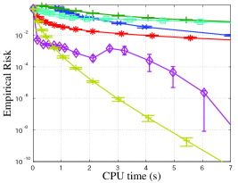
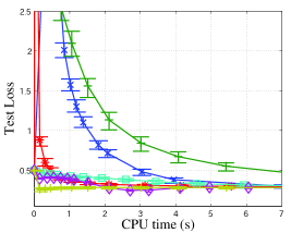
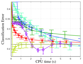
(a) $n=512$

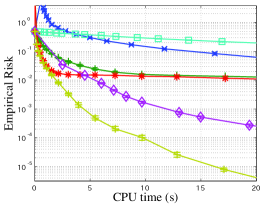
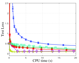
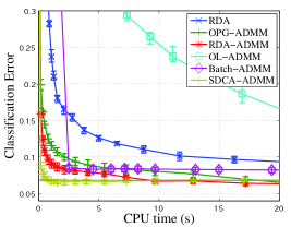
(b) $n=5120$

Figure 1: Artificial data: Excess empirical risk, exected loss on the test data and test classification error averaged over 10 independent iteration against CPU time in artificial data with (a) $n=512$ and (b) $n=5120$. The error bar indicates the standard deviation.

We observe that the excess empirical risk of our method, SDCA-ADMM, actually converges linearly while other stochastic methods don’t show linear convergence. Although Batch-ADMM also shows linear convergence and its convergence speed is comparable to SDCA-ADMM for small sample situation ($n=512$), SDCA-ADMM is much faster than Batch-ADMM when the number of samples is large ($n=5120$). As for the classification error, existing stochastic methods also show nice performances despite the poor convergence of the empirical risk. On the other hand, SDCA-ADMM rapidly converges to a stable state and shows comparable or better classification accuracy than existing methods.

6.2 Real Data

Here we execute numerical experiments on real data sets; ‘20 Newsgroups’ and ‘a9a’. ‘20 Newsgroups’ contains 100 dimensional 12,995 training samples and 3,247 test samples. ‘a9a’ contains 123 dimensional 32,561 training samples and 16,281 test samples. We constructed a similarity graph between features using graph Lasso and applied graph guided regularization as in Ouyang et al. (2013). That is, we applied graph Lasso to the training samples, and obtain a sparse inverse variance-covariance matrix $\hat{F}$. Based on the similarity matrix $\hat{F}$, we connect all index pairs $(i,j)$ with $\hat{F}_{i,j}\neq 0$ on edges. We denote by $E$ the set of edges. Then we impose the following graph guided regularization:

$$\textstyle\tilde{\psi}(w)=C_{1}\sum_{i=1}^{p}|w_{i}|+C_{2}\sum_{(i,j)\in E}|w_{i}-w_{j}|+0.01\times(C_{1}\sum_{i=1}^{p}|w_{i}|^{2}+C_{2}\sum_{(i,j)\in E}|w_{i}-w_{j}|^{2}).$$

Now let $F$ be $|E|\times p$ matrix where $F_{e,i}=1$ and $F_{e,j}=-1$, if $(i,j)=e\in E$, and $F_{e,i}=0$ otherwise. Then by letting $B^{\top}=[\mathrm{I}_{p};F]$ and $\psi(u)=C_{1}\sum_{i=1}^{p}|u_{i}|+C_{2}\sum_{i=p+1}^{|E|}|u_{i}|+0.01(C_{1}\sum_{i=1}^{p}|u_{i}|^{2}+C_{2}\sum_{i=p+1}^{|E|}|u_{i}|^{2})$ for $u\in\mathbb{R}^{p+|E|}$, we have $\tilde{\psi}(w)=\psi(B^{\top}w)$. Note that the proximal operation with respect to $\psi$ is just the soft-thresholding operation. In our experiments, we employed $C_{2}=C_{1}|E|/p$ and $C_{1}=0.01/\sqrt{n}$.

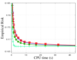
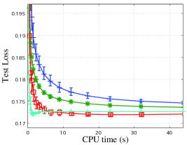
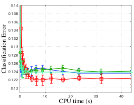
(a) 20news

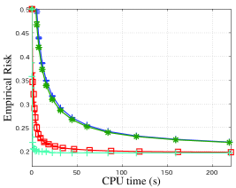
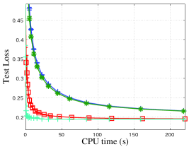
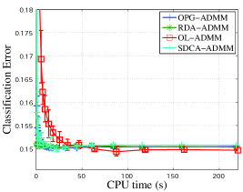
(b) a9a

Figure 2: Real data: Empirical risk, average loss on the test data and test classification error averaged over 5 independent iteration against CPU time in real data ((a) 20news, (b) a9a). The error bar indicates the standard deviation.

We computed the empirical risk on the training data, the averaged loss on the test data, and the test classification error (Figure 2). We observe that the empirical risk on the training data of SDCA-ADMM converges much faster than other methods. Although other methods also performs well on the test loss and the classification error, SDCA-ADMM still converges faster than existing methods with respect to the two quantities measured on the test data.

7 Conclusion

We proposed a new stochastic dual coordinate ascent technique with alternating direction multiplier method. The proposed method can be applied to wide range of regularization functions. Moreover, we proposed a mini-batch extension of our method. It is shown that, under some strong convexity conditions, our method converges exponentially. According to our analysis, the mini-batch method improves the convergence rate if the input features don’t have strong correlation between each other. The numerical experiments showed that our method actually converges exponentially, and the convergence is fast in terms of both empirical and expected risk.

Future work includes that the determination of $\eta_{Z,I}$. In Theorem 2, the exponential convergence is guaranteed if $\eta_{Z,I}>=(1+2\gamma n(1-1/K))\sigma_{\max}(Z_{I}^{\top}Z_{I})$. However, in our preliminary numerical experiments, an aggressive method like the one suggested in Takáč et al. (2013) performed effectively in some data sets. Developing more sophisticated determination of $\eta_{Z,I}$ (and $G$) would be a potentially promising future work.

Appendix A Appendix: Proof of Theorem 2

Here, we give the proof of Theorem 2. For notational simplicity, we rewrite the dual problem as follows:

$$\min_{x\in\mathcal{X},y\in\mathcal{Y}} ~{}~{}\sum_{i=1}^{n}g_{i}(x_{i})+\phi(y),$$ (17a)

$$\mathrm{s.t.} ~{}~{}Zx+By=0,$$ (17b)

where $Z\in\mathbb{R}^{p\times n}$, $B\in\mathbb{R}^{p\times d}$. This is equivalent to the dual optimization problem in the main text when $g_{i}=f_{i}^{*}$ and $\phi=n\psi^{*}(\cdot/n)$ (or equivalently $\phi^{*}=n\psi$). We write $g(x)=\sum_{i=1}^{n}g_{i}(x_{i})$.

Then we consider the following update rule:

$$y^{(t)} \leftarrow\mathop{\arg\min}_{y}\phi(y)-\langle w^{(t-1)},Zx^{(t-1)}+By\rangle+\frac{\rho}{2}\|Zx^{(t-1)}+By\|^{2}+\frac{1}{2}\|y-y^{(t-1)}\|_{Q}$$

$$x^{(t)}_{i} \leftarrow\mathop{\arg\min}_{x_{I}}\sum_{i\in I}g_{i}(x_{i})-\langle w^{(t-1)},Z_{I}x_{I}+By^{(t)}\rangle+\frac{\rho}{2}\|Z_{I}x_{I}+Z_{\backslash I}x^{(t-1)}_{\backslash I}+By^{(t)}\|^{2}+\frac{1}{2}\|x_{I}-x^{(t-1)}_{I}\|_{G_{ii}}$$

$$w^{(t)} =w^{(t-1)}-\gamma\rho\{n(Zx^{(t)}+By^{(t)})-(n-n/K)(Zx^{(t-1)}+By^{(t-1)})\}.$$

Assumption 1 can be interpreted as follows. There is an optimal solution $(x^{*},y^{*})$ and corresponding Lagrange multiplier $w^{*}$ such that

$$\nabla g(x^{*})=Z^{\top}w^{*},~{}~{}\nabla\phi(y^{*})\ni B^{\top}w^{*}.$$

Moreover, we suppose that each (dual) loss function $g_{i}$ is $v$-strongly convex and $\phi$ is $h$-smooth:

$$g_{i}(x_{i})-g_{i}(x_{i}^{*})\geq\langle\nabla g_{i}(x_{i}^{*}),x_{i}-x_{i}^{*}\rangle+\frac{v\|x_{i}-x_{i}^{*}\|^{2}}{2}.$$

We also assume that there exit $h$ and $v_{\phi}$ such that, for all $y,u$ and all $y^{*}\in\mathcal{Y}^{*}$, there exits $\widehat{y}^{*}\in\mathcal{Y}^{*}$ which depends on $y$ and we have

$$\phi(y)-\phi(y^{*})\geq\langle B^{\top}w^{*},y-y^{*}\rangle+\frac{v_{\phi}^{\prime}}{2}\|P_{\mathrm{Ker}(B)}(y-y^{*})\|^{2},$$

$$\phi^{*}(u)-\phi^{*}(B^{\top}w^{*})\geq\langle y^{*},u-B^{\top}w^{*}\rangle+\frac{h^{\prime}}{2}\|u-B^{\top}w^{*}\|^{2}.$$

Note that the primal and dual are flipped compared with the main text. Once can check that there is a correspondence between $v_{\psi},h$ in the main text and $v_{\phi}^{\prime}$ and $h^{\prime}$ such that $v_{\phi}^{\prime}=\frac{v_{\psi}}{n}$ and $h^{\prime}=nh$.

Define

$$F(x,y):=\sum_{i=1}^{n}g_{i}(x_{i})+\phi(y)-\langle w^{*},Zx+By\rangle~{}~{}~{}(=nF_{D}(x,y)).$$

By the definition of $w^{*}$, one can easily check that

$$F(x,y)-F(x^{*},y^{*})\geq\frac{nv}{2}\|x-x^{*}\|^{2}\geq 0.$$

We define

$$R^{\prime}(x,y,w)$$

$$= F(x,y)-F(x^{*},y^{*})+\frac{2}{\rho}\|w^{(t)}-w^{*}\|^{2}+\frac{\rho(1-\gamma)}{2}\|Zx+By\|^{2}+\frac{1}{2}\|x-x^{*}\|^{2}_{vI_{p}+H}+\frac{1}{2n}\|y-\mathcal{Y}^{*}\|^{2}_{Q}.$$

Here again we have that $R^{\prime}=nR_{D}$. Let $\hat{n}=n/K$, the expected cardinality of $|I|$, and let $\mathrm{Diag}_{\mathcal{I}}(S)$ be a block diagonal matrix whose $I_{k}\times I_{k}~{}(k=1,\dots,K)$ diagonal elements are non-zero and given by $(\mathrm{Diag}(S))_{I_{k},I_{k}}=S_{I_{k},I_{k}}$ ($k=1,\dots,K$).

Theorem 3.

Suppose that $\gamma=\frac{1}{4n}$, $\mathrm{Diag}_{\mathcal{I}}(G)\succ 2\gamma\rho(n-1)\mathrm{Diag}_{\mathcal{I}}(Z^{\top}Z)$ and $B^{\top}$ is injective. Then, under the assumptions, the objective function converges R-linearly:

$$R^{\prime}(x^{(t)},y^{(t)},w^{(t)})\leq\left(1-\frac{\mu}{K}\right)^{T}R(x^{(0)},y^{(0)},w^{(0)}),$$

$$\mathrm{E}[F(x^{(t)},y^{(t)})-F(x^{*},y^{*})]\leq\left(1-\frac{\mu}{K}\right)^{T}R(x^{(0)},y^{(0)},w^{(0)}),$$

where

$$\mu:=\min \Bigg{\{}\frac{1}{2}\left(\frac{v}{v+\sigma_{\max}(H)}\right),\frac{h^{\prime}\rho\sigma_{\min}(BB^{\top})}{2\max\{1,4h^{\prime}\rho,4h^{\prime}\sigma_{\max(Q)}\}},\frac{nv_{\phi}^{\prime}}{4\sigma_{\max(Q)}},\frac{nv\sigma_{\min}(BB^{\top})}{\sigma_{\max(Q)}(\rho\sigma_{\max}(Z^{\top}Z)+4v)}\Bigg{\}},$$

In particular, we have that

$$\mathrm{E}[\|w^{(t)}-w^{*}\|^{2}]\leq\frac{\rho}{2}\left(1-\frac{\mu}{K}\right)^{T}R(x^{(0)},y^{(0)},w^{(0)}).$$

Theorem 1 in the main text can be obtained using the relation $v_{\phi}^{\prime}=\frac{v_{\phi}}{n}$, $h^{\prime}=nh$, $F=nF_{D}$ and $R^{\prime}=nR_{D}$. The convergence of the primal objective is obtained by using the following fact: Since $g$ is strongly convex, we have that

$$g(x)-g(x^{*})\geq\langle\nabla g(x^{*}),x-x^{*}\rangle+\frac{v\|x-x^{*}\|^{2}}{2}~{}~{}(\forall x)$$

$$\Rightarrow g^{*}(u)\leq g^{*}(u^{*})+\langle\nabla g^{*}(u^{*}),u-u^{*}\rangle+\frac{\|u-u^{*}\|^{2}}{2v}~{}~{}(\forall v),$$

where $u^{*}\in\nabla g(x^{*})$. Using this, we have that,

$$\frac{1}{n}\sum_{i=1}^{n}f_{i}(z_{i}^{\top}w^{(t)})-\frac{1}{n}\sum_{i=1}^{n}f_{i}(z_{i}^{\top}w^{*}) \leq\left\langle Z\nabla\left(\frac{1}{n}\sum_{i=1}^{n}f_{i}\right)(u)\big{|}_{u=Z^{\top}w^{*}},w^{(t)}-w^{*}\right\rangle+\frac{\|Z^{\top}(w^{(t)}-w^{*})\|^{2}}{2nv}$$

$$=\left\langle-y^{*}/n,B^{\top}(w^{(t)}-w^{*})\right\rangle+\frac{\|Z^{\top}(w^{(t)}-w^{*})\|^{2}}{2nv},$$

where we used the relation $Zx^{*}+By^{*}=0$. Moreover, using the relation $\psi(B^{\top}w)\leq\psi(B^{\top}w^{*})+\langle y^{*}/n,B^{\top}(w-w^{*})\rangle+l_{1}\|w-w^{*}\|+l_{2}\|w-w^{*}\|^{2}$ and the Jensen’s inequality $\mathrm{E}[\|w^{(T)}-w^{*}\|]^{2}\leq\mathrm{E}[\|w^{(T)}-w^{*}\|^{2}]$, we obtain the assertion.

Proof of Theorem 3.

Step 1 (Deriving a basic inequality):

$$g(x^{(t)})-g(x^{(t-1)})+\phi(y^{(t)})-\phi(y^{(t-1)})$$

$$= \sum_{i\in I}g_{i}(x^{(t)}_{i})-\sum_{i\in I}g_{i}(x^{(t-1)}_{i})+\phi(y^{(t)})-\phi(y^{(t-1)})$$

$$= \sum_{i\in I}g_{i}(x^{(t)}_{i})-\langle w^{(t-1)},Zx^{(t)}+By^{(t)}\rangle+\frac{\rho}{2}\|Zx^{(t)}+By^{(t)}\|^{2}+\frac{1}{2}\|x^{(t)}_{I}-x^{(t-1)}_{I}\|_{G_{I,I}}^{2}$$

$$+\langle w^{(t-1)},Zx^{(t)}+By^{(t)}\rangle-\frac{\rho}{2}\|Zx^{(t)}+By^{(t)}\|^{2}-\frac{1}{2}\|x^{(t)}_{I}-x^{(t-1)}_{I}\|_{G_{I,I}}^{2}$$

$$-\sum_{i\in I}g_{i}(x^{(t-1)}_{i})+\phi(y^{(t)})-\phi(y^{(t-1)}).$$ (18)

Here we define that $\tilde{Z}_{I}=[Z_{\backslash I}Z_{I}]$ and $\tilde{x}:=\begin{bmatrix}x^{(t-1)}_{\backslash I}\\ x_{I}\end{bmatrix}$ for a given $x_{I}$, and

$$\tilde{g}_{I}(x_{I}):=\sum_{i\in I}g_{i}(x_{i})-\left\langle w^{(t-1)},\tilde{Z}_{I}\tilde{x}+By^{(t)}\right\rangle+\frac{\rho}{2}\|\tilde{Z}_{I}\tilde{x}+By^{(t)}\|^{2}+\frac{1}{2}\|x_{I}-x^{(t-1)}_{I}\|_{G_{I,I}}^{2}.$$

Then by the update rule of $x^{(t)}$, we have that

$$\tilde{g}_{I}(x^{(t)}_{I})\leq\tilde{g}_{I}(x^{*}_{I})-\frac{v}{2}\|x^{(t)}_{I}-x^{*}_{I}\|^{2}-\frac{\rho}{2}\|Z_{I}(x^{(t)}_{I}-x^{*}_{I})\|^{2}-\frac{1}{2}\|x^{(t)}_{I}-x^{*}_{I}\|_{G_{I,I}},$$

which implies

$$\sum_{i\in I}g_{i}(x^{(t)}_{i})-\left\langle w^{(t-1)},Zx^{(t)}+By^{(t)}\right\rangle+\frac{\rho}{2}\|Zx^{(+)}By^{(t)}\|^{2}+\frac{1}{2}\|x^{(t)}_{I}-x^{(t-1)}_{I}\|_{G_{I,I}}^{2}$$

$$\leq \sum_{i\in I}g_{i}(x^{*}_{i})-\left\langle w^{(t-1)},Z_{I}x^{*}_{I}+Z_{\backslash I}x^{*}_{\backslash I}+By^{(t)}\right\rangle+\frac{\rho}{2}\|Z_{I}x^{*}_{I}+Z_{\backslash I}x^{(t-1)}_{\backslash I}+By^{(t)}\|^{2}+\frac{1}{2}\|x^{*}_{I}-x^{(t-1)}_{I}\|_{G_{I,I}}^{2}$$

$$-\frac{v}{2}\|x^{(t)}_{I}-x^{*}_{I}\|^{2}-\frac{\rho}{2}\|Z_{I}(x^{(t)}_{I}-x^{*}_{I})\|^{2}-\frac{1}{2}\|x^{(t)}_{I}-x^{*}_{I}\|_{G_{I,I}}$$

$$= \sum_{i\in I}g_{i}(x^{*}_{i})-\left\langle w^{(t-1)},Z_{I}(x^{*}_{I}-x^{(t)}_{I})\right\rangle-\left\langle w^{(t-1)},Zx^{(t)}+By^{(t)}\right\rangle$$

$$+\frac{\rho}{2}\|Z_{I}x^{*}_{I}+Z_{\backslash I}x^{(t-1)}_{\backslash I}+By^{(t)}\|^{2}-\frac{\rho}{2}\|Zx^{(t)}+By^{(t)}\|^{2}+\frac{\rho}{2}\|Zx^{(t)}+By^{(t)}\|^{2}+\frac{1}{2}\|x^{*}_{I}-x^{(t-1)}_{I}\|_{G_{I,I}}^{2}$$

$$-\frac{v}{2}\|x^{(t)}_{I}-x^{*}_{I}\|^{2}-\frac{\rho}{2}\|Z_{I}(x^{(t)}_{I}-x^{*}_{I})\|^{2}-\frac{1}{2}\|x^{(t)}_{I}-x^{*}_{I}\|_{G_{I,I}}$$

$$= \sum_{i\in I}g_{i}(x^{*}_{i})-\left\langle w^{(t-1)},Z_{I}(x^{*}_{I}-x^{(t)}_{I})\right\rangle$$

$$-\frac{v}{2}\|x^{(t)}_{I}-x^{*}_{I}\|^{2}-\frac{\rho}{2}\|Z_{I}(x^{(t)}_{I}-x^{*}_{I})\|^{2}-\frac{1}{2}\|x^{(t)}_{I}-x^{*}_{I}\|_{G_{I,I}}$$

$$-\rho\langle Z_{\backslash I}x^{(t)}_{\backslash I}+By^{(t)},Z_{I}(x^{(t)}_{I}-x^{*}_{I})\rangle+\frac{\rho}{2}\|Z_{I}x^{*}_{I}\|^{2}-\frac{\rho}{2}\|Z_{I}x^{(t)}_{I}\|^{2}+\frac{1}{2}\|x^{*}_{I}-x^{(t-1)}_{I}\|_{G_{I,I}}^{2}$$

$$-\left\langle w^{(t-1)},Zx^{(t)}+By^{(t)}\right\rangle+\frac{\rho}{2}\|Zx^{(t-1)}+By^{(t)}\|^{2}.$$

Using this, the RHS of Eq. (18) can be further bounded by

$$\text{(RHS)}\leq \sum_{i\in I}g_{i}(x^{*}_{i})-\sum_{i\in I}g_{i}(x^{(t-1)}_{i})-\langle w^{(t-1)},Z_{I}(x^{*}_{I}-x^{(t)}_{I})\rangle$$

$$-\frac{v}{2}\|x^{(t)}_{I}-x^{*}_{I}\|^{2}-\frac{\rho}{2}\|Z_{I}(x^{(t)}_{I}-x^{*}_{I})\|^{2}-\frac{1}{2}\|x^{(t)}_{I}-x^{*}_{I}\|_{G_{I,I}}$$

$$-\rho\langle Z_{\backslash I}x^{(t)}_{\backslash I}+By^{(t)},Z_{I}(x^{(t)}_{I}-x^{*}_{I})\rangle+\frac{\rho}{2}\|Z_{I}x^{*}_{I}\|^{2}-\frac{\rho}{2}\|Z_{I}x^{(t)}_{I}\|^{2}$$

$$+\frac{1}{2}\|x^{*}_{I}-x^{(t-1)}_{I}\|_{G_{I,I}}^{2}-\frac{1}{2}\|x^{(t)}_{I}-x^{(t-1)}_{I}\|_{G_{I,I}}^{2}$$

$$+\phi(y^{(t)})-\phi(y^{(t-1)}).$$ (19)

Here, we bound the term

$$-\rho\langle Z_{\backslash i}x^{(t)}_{\backslash i}+By^{(t)},Z_{I}(x^{(t)}_{I}-x^{*}_{I})\rangle+\frac{\rho}{2}\|Z_{I}x^{*}_{I}\|^{2}-\frac{\rho}{2}\|Z_{I}x^{(t)}_{I}\|^{2}.$$

By Lemma 4, the expectation of this term is equivalent to

$$\mathrm{E}\left[-\frac{\rho}{n}\langle Zx^{(t-1)}+By^{(t)},Z(nx^{(t)}-(n-\hat{n})x^{(t-1)}-\hat{n}x^{*})\rangle\right]$$

$$+\frac{\rho}{2K}\|x^{(t-1)}-x^{*}\|^{2}_{\mathrm{Diag}_{\mathcal{I}}(Z^{\top}Z)}-\frac{\rho}{2}\mathrm{E}\left[\|x^{(t)}-x^{(t-1)}\|^{2}_{\mathrm{Diag}_{\mathcal{I}}(Z^{\top}Z)}\right].$$

Note that, for any block diagonal matrix $S$ which satisfies $S_{I_{k},I_{k^{\prime}}}=(S_{i,j})_{(i,j)\in I_{k}\times I_{k^{\prime}}}=O~{}(\forall k\neq k^{\prime})$, we have that

$$\mathrm{E}[\|x^{(t)}_{I}-x^{*}_{I}\|^{2}_{S_{I,I}}] =\mathrm{E}[\|x^{(t)}_{I}-x^{(t-1)}_{I}+x^{(t-1)}_{I}-x^{*}_{I}\|^{2}_{S_{I,I}}]$$

$$=\mathrm{E}[\|x^{(t)}_{I}-x^{(t-1)}_{I}\|^{2}_{S_{I,I}}]+\mathrm{E}[2\langle x^{(t)}_{I}-x^{(t-1)}_{I},x^{(t-1)}_{I}-x^{*}_{I}\rangle_{S_{I,I}}]+\mathrm{E}[\|x^{(t-1)}_{I}-x^{*}_{I}\|^{2}_{S_{I,I}}]$$

$$=\mathrm{E}[\|x^{(t)}-x^{(t-1)}\|^{2}_{S}]+\mathrm{E}[2\langle x^{(t)}-x^{(t-1)},x^{(t-1)}-x^{*}\rangle_{S}]+\frac{1}{K}\|x^{(t-1)}-x^{*}\|^{2}_{S}$$

$$=\mathrm{E}[\|x^{(t)}-x^{*}\|^{2}_{S}]-\mathrm{E}[\|x^{(t-1)}-x^{*}\|^{2}_{S}]+\frac{1}{K}\|x^{(t-1)}-x^{*}\|^{2}_{S}$$

$$=\mathrm{E}[\|x^{(t)}-x^{*}\|^{2}_{S}]-\left(1-\frac{1}{K}\right)\mathrm{E}[\|x^{(t-1)}-x^{*}\|^{2}_{S}],$$

where the expectation is taken with respect to the choice of $I\in\{I_{1},\dots,I_{K}\}$. Moreover, for a fixed vector $q$, we have that

$$\mathrm{E}[\langle q_{I},x^{(t)}_{I}-x^{*}_{I}\rangle]$$

$$= \mathrm{E}[\langle q_{I},x^{(t)}_{I}-x^{(t-1)}_{I}+x^{(t-1)}_{I}-x^{*}_{I}\rangle]=\mathrm{E}[\langle q,x^{(t)}-x^{(t-1)}\rangle]+\mathrm{E}[\langle q_{I},x^{(t-1)}_{I}-x^{*}_{I}\rangle]$$

$$= \mathrm{E}[\langle q,x^{(t)}-x^{(t-1)}\rangle]+\mathrm{E}\left[\sum_{k=1}^{K}1[I=I_{k}]\langle q_{I_{k}},x^{(t-1)}_{I_{k}}-x^{*}_{I_{k}}\rangle\right]$$

$$= \mathrm{E}[\langle q,x^{(t)}-x^{(t-1)}\rangle]+\frac{1}{K}\sum_{k=1}^{K}1[I=I_{k}]\langle q_{I_{k}},x^{(t-1)}_{I_{k}}-x^{*}_{I_{k}}\rangle=\mathrm{E}[\langle q,x^{(t)}-x^{(t-1)}\rangle]+\frac{1}{K}\langle q,x^{(t-1)}-x^{*}\rangle$$

$$= \mathrm{E}\left[\left\langle q,x^{(t)}-\left(1-\frac{1}{K}\right)x^{(t-1)}-\frac{1}{K}x^{*}\right\rangle\right].$$

Then, by taking expectation with respect to $I$ and multiplying both sides of the above inequality by $n$, we have that

$$n\mathrm{E}[g(x^{(t)})+\phi(y^{(t)})-g(x^{(t-1)})-\phi(y^{(t-1)})]$$

$$\leq g(x^{*})-g(x^{(t-1)})+\mathrm{E}[\langle w^{(t-1)},Z(nx^{(t)}-(n-\hat{n})x^{(t-1)}-\hat{n}x^{*})\rangle]$$

$$-\mathrm{E}\left[\frac{nv}{2}\|x^{(t)}-x^{*}\|^{2}+\frac{n\rho}{2}\|x^{(t)}-x^{*}\|_{\mathrm{Diag}_{\mathcal{I}}(Z^{\top}Z)}^{2}+\frac{n}{2}\|x^{(t)}-x^{*}\|_{\mathrm{Diag}_{\mathcal{I}}(G)}^{2}\right]$$

$$+\frac{(n-\hat{n})v}{2}\|x^{(t-1)}-x^{*}\|^{2}]+\frac{(n-\hat{n})\rho}{2}\|x^{(t-1)}-x^{*}\|_{\mathrm{Diag}_{\mathcal{I}}(Z^{\top}Z)}^{2}+\frac{n-\hat{n}}{2}\|x^{(t-1)}-x^{*}\|_{\mathrm{Diag}_{\mathcal{I}}(G)}^{2}$$

$$+\mathrm{E}\left[-\rho\langle Zx^{(t-1)}+By^{(t)},Z(nx^{(t)}-(n-\hat{n})x^{(t-1)}-\hat{n}x^{*})\rangle\right]$$

$$+\frac{\rho\hat{n}}{2}\|x^{(t-1)}-x^{*}\|^{2}_{\mathrm{Diag}_{\mathcal{I}}(Z^{\top}Z)}-\frac{n\rho}{2}\mathrm{E}\left[\|x^{(t)}-x^{(t-1)}\|^{2}_{\mathrm{Diag}_{\mathcal{I}}(Z^{\top}Z)}\right]$$

$$+\frac{\hat{n}}{2}\|x^{(t-1)}-x^{*}\|^{2}_{\mathrm{Diag}_{\mathcal{I}}(G)}-\frac{n}{2}\mathrm{E}[\|x^{(t)}-x^{(t-1)}\|^{2}_{\mathrm{Diag}_{\mathcal{I}}(G)}]$$

$$+n\phi(y^{(t)})-n\phi(y^{(t-1)}).$$ (20)

Here, note that the last two term $n\phi(y^{(t)})-n\phi(y^{(t-1)})$ is bounded as

$$n\phi(y^{(t)})-n\phi(y^{(t-1)})$$

$$= \hat{n}(\phi(y^{(t)})-\phi(y^{(t-1)}))+(n-\hat{n})(\phi(y^{(t)})-\phi(y^{(t-1)}))$$

$$\leq \hat{n}(\phi(y^{*})-\phi(y^{(t-1)}))+\left\langle\nabla\phi(y^{(t)}),(n-\hat{n})(y^{(t)}-y^{(t-1)})+\hat{n}(y^{(t)}-y^{*})\right\rangle$$

$$-\frac{\hat{n}h^{\prime}}{2}\|B^{\top}w^{*}-\nabla\phi(y^{(t)})\|^{2}.$$

for arbitrary $y^{*}\in\mathcal{Y}^{*}$ where we used Lemma 5 in the last line. Define

$$\tilde{w}^{(t)}:=w^{(t-1)}-\rho(Zx^{(t-1)}+By^{(t)}).$$

Note that $B^{\top}\tilde{w}^{(t)}-Q(y^{(t)}-y^{(t-1)})\in\nabla\phi(y^{(t)})$.

Next, adding $\mathrm{E}[n\langle w^{*},Z(x^{(t-1)}-x^{(t)})+B(y^{(t-1)}-y^{(t)})\rangle]$ to the both sides of Eq. (20), we have that

$$n\mathrm{E}[F(x^{(t)},y^{(t)})-F(x^{(t-1)},y^{(t-1)})]$$

$$\leq \hat{n}(F(x^{*},y^{*})-F(x^{(t-1)},y^{(t-1)}))$$

$$+\mathrm{E}[\langle w^{(t-1)}-w^{*},Z(nx^{(t)}-(n-\hat{n})x^{(t-1)}-\hat{n}x^{*})\rangle]$$

$$+\mathrm{E}[\langle\tilde{w}^{(t)}-w^{*},B(ny^{(t)}-(n-\hat{n})y^{(t-1)}-\hat{n}y^{*})\rangle]$$

$$-\langle Q(y^{(t)}-y^{(t-1)}),ny^{(t)}-(n-\hat{n})y^{(t-1)}-\hat{n}y^{*}\rangle$$

$$-\mathrm{E}\left[\frac{nv}{2}\|x^{(t)}-x^{*}\|^{2}+\frac{n}{2}\|x^{(t)}-x^{*}\|_{H}^{2}\right]$$

$$+\frac{(n-\hat{n})v}{2}\|x^{(t-1)}-x^{*}\|^{2}+\frac{n}{2}\|x^{(t-1)}-x^{*}\|_{H}^{2}$$

$$+\mathrm{E}\left[-\rho\langle Zx^{(t-1)}+By^{(t)},Z(nx^{(t)}-(n-\hat{n})x^{(t-1)}-\hat{n}x^{*})\rangle\right]$$

$$-\frac{n}{2}\mathrm{E}\left[\|x^{(t)}-x^{(t-1)}\|^{2}_{H}\right]-\frac{\hat{n}h^{\prime}}{2}\|B^{\top}w^{*}-\nabla\phi(y^{(t)})\|^{2}.$$ (21)

Step 2 (Rearranging cross terms between $(x^{(t)},y^{(t)},w^{(t)})$ and $(x^{(t-1)},y^{(t-1)},w^{(t-1)})$):

Now, we define $\hat{x}^{(t)}:=nx^{(t)}-(n-\hat{n})x^{(t-1)}$ and $\hat{y}^{(t)}:=ny^{(t)}-(n-\hat{n})y^{(t-1)}$. Then by the update rule of $w^{(t)}$, we have that $w^{(t)}=w^{(t-1)}-\gamma\rho(Z\hat{x}^{(t)}+B\hat{y}^{(t)})$. We evaluate the term $\mathrm{E}[\langle w^{(t-1)}-w^{*},Z(\hat{x}^{(t)}-\hat{n}x^{*})\rangle]+\mathrm{E}[\langle\tilde{w}^{(t)}-w^{*},B(\hat{y}^{(t)}-\hat{n}y^{*})\rangle]$:

$$\langle w^{(t-1)}-w^{*},Z(\hat{x}^{(t)}-\hat{n}x^{*})\rangle+\langle\tilde{w}^{(t)}-w^{*},B(\hat{y}^{(t)}-\hat{n}y^{*})\rangle$$

$$= \langle w^{(t-1)}-w^{*},Z(\hat{x}^{(t)}-\hat{n}x^{*})\rangle+\langle w^{(t-1)}-\rho(Zx^{(t-1)}+By^{(t)})-w^{*},B(\hat{y}^{(t)}-\hat{n}y^{*})\rangle$$

$$= \langle w^{(t)}+\gamma\rho(Z\hat{x}^{(t)}+B\hat{y}^{(t)})-w^{*},Z(\hat{x}^{(t)}-\hat{n}x^{*})\rangle$$

$$+\langle w^{(t)}+\gamma\rho(Z\hat{x}^{(t)}+B\hat{y}^{(t)})-\rho(Zx^{(t-1)}+By^{(t)})-w^{*},B(\hat{y}^{(t)}-\hat{n}y^{*})\rangle$$

$$= -\frac{1}{\gamma\rho}\langle w^{(t)}-w^{*},w^{(t)}-w^{(t-1)}\rangle$$

$$+\gamma\rho\|Z\hat{x}^{(t)}+B\hat{y}^{(t)}\|^{2}-\rho\langle Zx^{(t-1)}+By^{(t)},B(\hat{y}^{(t)}-\hat{n}y^{*})\rangle$$

$$= -\frac{1}{2\gamma\rho}\left(\|w^{(t)}-w^{*}\|^{2}+\|w^{(t)}-w^{(t-1)}\|^{2}-\|w^{(t-1)}-w^{*}\|^{2}\right)$$

$$+\gamma\rho\|Z\hat{x}^{(t)}+B\hat{y}^{(t)}\|^{2}-\rho\langle Zx^{(t-1)}+By^{(t)},B(\hat{y}^{(t)}-\hat{n}y^{*})\rangle$$

$$= \frac{1}{2\gamma\rho}\left(-\|w^{(t)}-w^{*}\|^{2}+\|w^{(t-1)}-w^{*}\|^{2}\right)+\frac{\gamma\rho}{2}\|Z\hat{x}^{(t)}+B\hat{y}^{(t)}\|^{2}$$

$$-\rho\langle Zx^{(t-1)}+By^{(t)},B(\hat{y}^{(t)}-\hat{n}y^{*})\rangle.$$

Therefore,

$$\langle w^{(t-1)}-w^{*},Z(\hat{x}^{(t)}-\hat{n}x^{*})+\langle\tilde{w}^{(t)}-w^{*},B(\hat{y}^{(t)}-\hat{n}y^{*})\rangle$$

$$-\rho\langle Zx^{(t-1)}+By^{(t)},Z(nx^{(t)}-(n-\hat{n})x^{(t-1)}-\hat{n}x^{*})\rangle$$

$$= \frac{1}{2\gamma\rho}\left(-\|w^{(t)}-w^{*}\|^{2}+\|w^{(t-1)}-w^{*}\|^{2}\right)+\frac{\gamma\rho}{2}\|Z\hat{x}^{(t)}+B\hat{y}^{(t)}\|^{2}$$

$$-\rho\langle Zx^{(t-1)}+By^{(t)},Z\hat{x}^{(t)}+B\hat{y}^{(t)}\rangle$$

$$= \frac{1}{2\gamma\rho}\left(-\|w^{(t)}-w^{*}\|^{2}+\|w^{(t-1)}-w^{*}\|^{2}\right)$$

$$+\frac{\gamma\rho}{2}n^{2}\|Zx^{(t)}+By^{(t)}\|^{2}+\frac{\gamma\rho}{2}(n-\hat{n})^{2}\|Zx^{(t-1)}+By^{(t-1)}\|^{2}$$

$$-\gamma\rho n(n-\hat{n})\langle Zx^{(t)}+By^{(t)},Zx^{(t-1)}+By^{(t-1)}\rangle$$

$$-\rho\langle Zx^{(t-1)}+By^{(t)},Z(nx^{(t)}-(n-\hat{n})x^{(t-1)})+B(ny^{(t)}-(n-\hat{n})y^{(t-1)})\rangle.$$

Next, we expand the non-squared term:

$$-\gamma\rho n(n-\hat{n})\langle Zx^{(t)}+By^{(t)},Zx^{(t-1)}+By^{(t-1)}\rangle$$

$$-\rho\langle Zx^{(t-1)}+By^{(t)},Z(nx^{(t)}-(n-\hat{n})x^{(t-1)})+B(ny^{(t)}-(n-\hat{n})y^{(t-1)})\rangle$$

$$= -\gamma\rho n(n-\hat{n})\langle Zx^{(t)}-Zx^{*},Zx^{(t-1)}-Zx^{*}\rangle$$

$$-\gamma\rho n(n-\hat{n})\langle By^{(t)}-By^{*},By^{(t-1)}-By^{*}\rangle$$

$$-\gamma\rho n(n-\hat{n})\langle Zx^{(t)}-Zx^{*},By^{(t-1)}-By^{*}\rangle$$

$$-\gamma\rho n(n-\hat{n})\langle By^{(t)}-By^{*},Zx^{(t-1)}-Zx^{*}\rangle$$

$$-n\rho\langle Zx^{(t-1)}-Zx^{*},Z(x^{(t)}-x^{*})\rangle+(n-\hat{n})\rho\|Zx^{(t-1)}-Zx^{*}\|^{2}$$

$$+(n-\hat{n})\rho\langle By^{(t)}-By^{*},B(y^{(t-1)}-y^{*})\rangle-n\rho\|By^{(t)}-By^{*}\|^{2}$$

$$-\rho\langle Zx^{(t-1)}-Zx^{*},B(ny^{(t)}-(n-\hat{n})y^{(t-1)}-\hat{n}y^{*})\rangle$$

$$-\rho\langle B(y^{(t)}-y^{*}),Z(nx^{(t)}-(n-\hat{n})x^{(t-1)}-\hat{n}x^{*})\rangle$$

$$= -(\gamma\rho n(n-\hat{n})+n\rho)\langle Zx^{(t)}-Zx^{*},Zx^{(t-1)}-Zx^{*}\rangle$$

$$-(\gamma\rho n(n-\hat{n})-(n-\hat{n})\rho)\langle By^{(t)}-By^{*},By^{(t-1)}-By^{*}\rangle$$

$$-\gamma\rho n(n-\hat{n})\langle Zx^{(t)}-Zx^{*},By^{(t-1)}-By^{*}\rangle$$

$$-(\gamma\rho n(n-\hat{n})+n\rho-(n-\hat{n})\rho)\langle By^{(t)}-By^{*},Zx^{(t-1)}-Zx^{*}\rangle$$

$$+(n-\hat{n})\rho\|Zx^{(t-1)}-Zx^{*}\|^{2}-n\rho\|By^{(t)}-By^{*}\|^{2}$$

$$-\rho(n-\hat{n})\langle Zx^{(t-1)}-Zx^{*},B(y^{*}-y^{(t-1)})\rangle$$

$$-\rho n\langle B(y^{(t)}-y^{*}),Z(x^{(t)}-x^{*})\rangle.$$ (22)

Using the relation

$$\langle Zx^{(t)}-Zx^{*},By^{(t-1)}-By^{*}\rangle=\langle Z(x^{(t)}-x^{*}),B(y^{(t)}-y^{*})\rangle+\langle Z(x^{(t)}-x^{*}),B(y^{(t-1)}-y^{(t)})\rangle,$$

$$\langle By^{(t)}-By^{*},Zx^{(t-1)}-Zx^{*}\rangle=\langle B(y^{(t)}-y^{(t-1)}),Z(x^{(t-1)}-x^{*})\rangle+\langle B(y^{(t-1)}-y^{*}),Z(x^{(t-1)}-x^{*})\rangle,$$

the RHS of Eq. (22) is equivalent to

$$-(\gamma\rho n(n-\hat{n})+n\rho)\langle Zx^{(t)}-Zx^{*},Zx^{(t-1)}-Zx^{*}\rangle$$

$$-(\gamma\rho n(n-\hat{n})-(n-\hat{n})\rho)\langle By^{(t)}-By^{*},By^{(t-1)}-By^{*}\rangle$$

$$+(n-\hat{n})\rho\|Zx^{(t-1)}-Zx^{*}\|^{2}-n\rho\|By^{(t)}-By^{*}\|^{2}$$

$$+\{-(\gamma\rho n(n-\hat{n})+\rho\hat{n})+\rho(n-\hat{n})\}\langle Zx^{(t-1)}-Zx^{*},B(y^{(t-1)}-y^{*})\rangle$$

$$-(\gamma\rho n(n-\hat{n})+\rho n)\langle B(y^{(t)}-y^{*}),Z(x^{(t)}-x^{*})\rangle$$

$$-\gamma\rho n(n-\hat{n})\langle Z(x^{(t)}-x^{*}),B(y^{(t-1)}-y^{(t)})\rangle$$

$$-(\gamma\rho n(n-\hat{n})+\rho\hat{n})\langle By^{(t)}-By^{(t-1)},Zx^{(t-1)}-Zx^{*}\rangle.$$

The last two terms are transformed to

$$-\gamma\rho n(n-\hat{n})\langle Z(x^{(t)}-x^{*}),B(y^{(t-1)}-y^{(t)})\rangle$$

$$-(\gamma\rho n(n-\hat{n})+\rho\hat{n})\langle By^{(t)}-By^{(t-1)},Zx^{(t-1)}-Zx^{*}\rangle$$

$$= \gamma\rho n(n-\hat{n})\langle Z(x^{(t)}-x^{(t-1)}),B(y^{(t)}-y^{(t-1)})\rangle$$

$$-\rho\hat{n}\langle By^{(t)}-By^{*},Zx^{(t-1)}-Zx^{*}\rangle+\rho\hat{n}\langle By^{(t-1)}-By^{*},Zx^{(t-1)}-Zx^{*}\rangle.$$

Thus, the RHS of Eq. (22) is further transformed to

$$-(\gamma\rho n(n-\hat{n})+n\rho)\langle Zx^{(t)}-Zx^{*},Zx^{(t-1)}-Zx^{*}\rangle$$

$$-(\gamma\rho n(n-\hat{n})-(n-\hat{n})\rho)\langle By^{(t)}-By^{*},By^{(t-1)}-By^{*}\rangle$$

$$+(n-\hat{n})\rho\|Zx^{(t-1)}-Zx^{*}\|^{2}-n\rho\|By^{(t)}-By^{*}\|^{2}$$

$$+\{-\gamma\rho n(n-\hat{n})+\rho(n-\hat{n})\}\langle Zx^{(t-1)}-Zx^{*},B(y^{(t-1)}-y^{*})\rangle$$

$$-(\gamma\rho n(n-\hat{n})+\rho n)\langle B(y^{(t)}-y^{*}),Z(x^{(t)}-x^{*})\rangle$$

$$+\gamma\rho n(n-\hat{n})\langle Z(x^{(t)}-x^{(t-1)}),B(y^{(t)}-y^{(t-1)})\rangle$$

$$-\rho\hat{n}\langle By^{(t)}-By^{*},Zx^{(t-1)}-Zx^{*}\rangle.$$

By Lemma 6 and $Zx^{*}=-By^{*}$, this is equivalent to

$$-\frac{1}{2}(\gamma\rho n(n-\hat{n})+n\rho)\{\|Zx^{(t)}-Zx^{*}\|^{2}+\|Zx^{(t-1)}-Zx^{*}\|^{2}-\|Zx^{(t)}-Zx^{(t-1)}\|^{2}\}$$

$$-\frac{1}{2}(\gamma\rho n(n-\hat{n})-(n-\hat{n})\rho)\{\|By^{(t)}-By^{*}\|^{2}+\|By^{(t-1)}-By^{*}\|^{2}-\|By^{(t)}-By^{(t-1)}\|^{2}\}$$

$$+(n-\hat{n})\rho\|Zx^{(t-1)}-Zx^{*}\|^{2}-n\rho\|By^{(t)}-By^{*}\|^{2}$$

$$-\frac{1}{2}\{-\gamma\rho n(n-\hat{n})+\rho(n-\hat{n})\}(\|Zx^{(t-1)}-Zx^{*}\|^{2}+\|B(y^{(t-1)}-y^{*})\|^{2}-\|Zx^{(t-1)}+By^{(t-1)}\|^{2})$$

$$+\frac{1}{2}(\gamma\rho n(n-\hat{n})+\rho n)(\|Zx^{(t)}-Zx^{*}\|^{2}+\|B(y^{(t)}-y^{*})\|^{2}-\|Zx^{(t)}+By^{(t)}\|^{2})$$

$$+\gamma\rho n(n-\hat{n})\langle Z(x^{(t)}-x^{(t-1)}),B(y^{(t)}-y^{(t-1)})\rangle$$

$$-\rho\hat{n}\langle By^{(t)}-By^{*},Zx^{(t-1)}-Zx^{*}\rangle$$

$$= -\frac{\rho\hat{n}}{2}\|Zx^{(t-1)}-Zx^{*}\|^{2}+\frac{1}{2}(\gamma\rho n(n-\hat{n})+n\rho)\|Zx^{(t)}-Zx^{(t-1)}\|^{2}$$

$$-\frac{\rho\hat{n}}{2}\|By^{(t)}-By^{*}\|^{2}+\frac{1}{2}(\gamma\rho n(n-\hat{n})-(n-\hat{n})\rho)\|By^{(t)}-By^{(t-1)}\|^{2}$$

$$-\frac{1}{2}\{\gamma\rho n(n-\hat{n})-\rho(n-\hat{n})\}\|Zx^{(t-1)}+By^{(t-1)}\|^{2}$$

$$-\frac{1}{2}\{\gamma\rho n(n-\hat{n})+\rho n\}\|Zx^{(t)}+By^{(t)}\|^{2}$$

$$+\gamma\rho n(n-\hat{n})\langle Z(x^{(t)}-x^{(t-1)}),B(y^{(t)}-y^{(t-1)})\rangle$$

$$-\hat{n}\rho\langle By^{(t)}-By^{*},Zx^{(t-1)}-Zx^{*}\rangle$$

$$= -\frac{\hat{n}\rho}{2}\|Zx^{(t-1)}+By^{(t)}\|^{2}$$

$$+\frac{1}{2}(\gamma\rho n(n-\hat{n})+n\rho)\|Zx^{(t)}-Zx^{(t-1)}\|^{2}$$

$$+\frac{1}{2}(\gamma\rho n(n-\hat{n})-(n-\hat{n})\rho)\|By^{(t)}-By^{(t-1)}\|^{2}$$

$$-\frac{1}{2}\{\gamma\rho n(n-\hat{n})-\rho(n-\hat{n})\}\|Zx^{(t-1)}+By^{(t-1)}\|^{2}$$

$$-\frac{1}{2}\{\gamma\rho n(n-\hat{n})+\rho n\}\|Zx^{(t)}+By^{(t)}\|^{2}$$

$$+\gamma\rho n(n-\hat{n})\langle Z(x^{(t)}-x^{(t-1)}),B(y^{(t)}-y^{(t-1)})\rangle.$$ (23)

Since

$$\gamma\rho n(n-\hat{n})\langle Z(x^{(t)}-x^{(t-1)}),B(y^{(t)}-y^{(t-1)})\rangle$$

$$\leq \frac{\gamma\rho n(n-\hat{n})}{2}\{\|Z(x^{(t)}-x^{(t-1)})\|^{2}+\|B(y^{(t)}-y^{(t-1)})\|^{2}\},$$

the RHS of Eq. (23) is bounded by

$$-\frac{\hat{n}\rho}{2}\|Zx^{(t-1)}+By^{(t)}\|^{2}$$

$$+\frac{1}{2}(2\gamma\rho n(n-\hat{n})+n\rho)\|Zx^{(t)}-Zx^{(t-1)}\|^{2}$$

$$+\frac{1}{2}(2\gamma\rho n(n-\hat{n})-(n-\hat{n})\rho)\|By^{(t)}-By^{(t-1)}\|^{2}$$

$$-\frac{1}{2}\{\gamma\rho n(n-\hat{n})-\rho(n-\hat{n})\}\|Zx^{(t-1)}+By^{(t-1)}\|^{2}-\frac{1}{2}\{\gamma\rho n(n-\hat{n})+\rho n\}\|Zx^{(t)}+By^{(t)}\|^{2}.$$

Combining this and Eq. (21), and noticing $\|Zx^{(t)}-Zx^{(t-1)}\|=\|Z_{I}(x^{(t)}_{I}-x^{(t-1)}_{I})\|=\|x^{(t)}-x^{(t-1)}\|_{\mathrm{Diag}_{\mathcal{I}}(Z^{\top}Z)}$, we obtain

$$n\mathrm{E}[F(x^{(t)},y^{(t)})-F(x^{(t-1)},y^{(t-1)})]$$

$$\leq \hat{n}(F(x^{*},y^{*})-F(x^{(t-1)},y^{(t-1)}))$$

$$+\frac{1}{2\gamma\rho}\left(-\|w^{(t)}-w^{*}\|^{2}+\|w^{(t-1)}-w^{*}\|^{2}\right)$$

$$-\frac{\hat{n}\rho}{2}\|Zx^{(t-1)}+By^{(t)}\|^{2}$$

$$+\frac{1}{2}\{\gamma\rho n^{2}-\gamma\rho n(n-\hat{n})-\rho n\}\|Zx^{(t)}+By^{(t)}\|^{2}$$

$$+\frac{1}{2}\{\gamma\rho(n-\hat{n})^{2}-\gamma\rho n(n-\hat{n})+\rho(n-\hat{n})\}\|Zx^{(t-1)}+By^{(t-1)}\|^{2}$$

$$-\mathrm{E}\left[\frac{nv}{2}\|x^{(t)}-x^{*}\|^{2}+\frac{n}{2}\|x^{(t)}-x^{*}\|_{H}^{2}\right]$$

$$+\frac{(n-\hat{n})v}{2}\|x^{(t-1)}-x^{*}\|^{2}+\frac{n}{2}\|x^{(t-1)}-x^{*}\|_{H}^{2}$$

$$+\gamma\rho n(n-\hat{n})\mathrm{E}\left[\|x^{(t)}-x^{(t-1)}\|^{2}_{\mathrm{Diag}_{\mathcal{I}}(Z^{\top}Z)}\right]-\frac{n}{2}\mathrm{E}[\|x^{(t)}-x^{(t-1)}\|^{2}_{\mathrm{Diag}_{\mathcal{I}}(G)}]$$

$$+(\gamma\rho n(n-\hat{n})-\frac{(n-\hat{n})\rho}{2})\|B(y^{(t)}-y^{(t-1)})\|^{2}$$

$$-\langle Q(y^{(t)}-y^{(t-1)}),ny^{(t)}-(n-\hat{n})y^{(t-1)}-\hat{n}y^{*}\rangle$$

$$-\frac{\hat{n}h^{\prime}}{2}\|B^{\top}w^{*}-\nabla\phi(y^{(t)})\|^{2}.$$

Since we have assumed $\mathrm{Diag}_{\mathcal{I}}(G)\succ 2\gamma\rho(n-\hat{n})\mathrm{Diag}_{\mathcal{I}}(Z^{\top}Z)$, it holds that

$$\gamma\rho n(n-\hat{n})\mathrm{E}\left[\|x^{(t)}-x^{(t-1)}\|^{2}_{\mathrm{Diag}_{\mathcal{I}}(Z^{\top}Z)}\right]-\frac{n}{2}\mathrm{E}[\|x^{(t)}-x^{(t-1)}\|^{2}_{\mathrm{Diag}_{\mathcal{I}}(G)}]\leq 0.$$

Moreover, we have that

$$-\langle Q(y^{(t)}-y^{(t-1)}),ny^{(t)}-(n-\hat{n})y^{(t-1)}-\hat{n}y^{*}\rangle$$

$$= -n\|y^{(t)}-y^{(t-1)}\|_{Q}^{2}+\frac{1}{2}\{\|y^{(t)}-y^{(t-1)}\|^{2}_{Q}+\|y^{(t-1)}-y^{*}\|^{2}_{Q}-\|y^{(t)}-y^{*}\|^{2}_{Q}\}$$

$$= -\left(n-\frac{\hat{n}}{2}\right)\|y^{(t)}-y^{(t-1)}\|_{Q}^{2}+\frac{\hat{n}}{2}\|y^{(t-1)}-y^{*}\|^{2}_{Q}-\frac{\hat{n}}{2}\|y^{(t)}-y^{*}\|^{2}_{Q}.$$

Finally, we achieve

$$n\mathrm{E}[F(x^{(t)},y^{(t)})-F(x^{(t-1)},y^{(t-1)})]$$

$$\leq \hat{n}(F(x^{*},y^{*})-F(x^{(t-1)},y^{(t-1)}))$$

$$+\frac{1}{2\gamma\rho}\left(-\|w^{(t)}-w^{*}\|^{2}+\|w^{(t-1)}-w^{*}\|^{2}\right)$$

$$-\frac{\rho n(1-\gamma)}{2}\|Zx^{(t)}+By^{(t)}\|^{2}+\frac{\rho(n-\hat{n})(1+\gamma)}{2}\|Zx^{(t-1)}+By^{(t-1)}\|^{2}$$

$$-\mathrm{E}\left[\frac{nv}{2}\|x^{(t)}-x^{*}\|^{2}+\frac{n}{2}\|x^{(t)}-x^{*}\|_{H}^{2}\right]$$

$$+\frac{(n-\hat{n})v}{2}\|x^{(t-1)}-x^{*}\|^{2}+\frac{n\rho}{2}\|x^{(t-1)}-x^{*}\|_{H}^{2}$$

$$+\gamma\rho n(n-\hat{n})\mathrm{E}\left[\|x^{(t)}-x^{(t-1)}\|^{2}_{\mathrm{Diag}_{\mathcal{I}}(Z^{\top}Z)}\right]-\frac{n}{2}\mathrm{E}[\|x^{(t)}-x^{(t-1)}\|^{2}_{\mathrm{Diag}_{\mathcal{I}}(G)}]$$

$$-\frac{\hat{n}\rho}{2}\|Zx^{(t-1)}+By^{(t)}\|^{2}$$

$$+(\gamma\rho n(n-\hat{n})-\frac{(n-\hat{n})\rho}{2})\|B(y^{(t)}-y^{(t-1)})\|^{2}$$

$$-\left(n-\frac{\hat{n}}{2}\right)\|y^{(t)}-y^{(t-1)}\|_{Q}^{2}+\frac{\hat{n}}{2}\|y^{(t-1)}-y^{*}\|^{2}_{Q}-\frac{\hat{n}}{2}\|y^{(t)}-y^{*}\|^{2}_{Q}$$

$$-\frac{\hat{n}h^{\prime}}{2}\|B^{\top}w^{*}-\nabla\phi(y^{(t)})\|^{2}.$$ (24)

Note that Eq. (24) holds for arbitrary $y^{*}\in\mathcal{Y}^{*}$.

Step 3: (Deriving the assertion)

(i) Now, since $\nabla\phi(y^{(t)})=B^{\top}w^{(t-1)}-\rho(Zx^{(t-1)}+By^{(t)})-Q(y^{(t)}-y^{(t-1)})$, it holds that

$$\|B^{\top}w^{*}-\nabla\phi(y^{(t)})\|^{2}=\|B^{\top}(w^{*}-w^{(t-1)})-\rho(Zx^{(t-1)}+By^{(t)})-Q(y^{(t)}-y^{(t-1)})\|^{2}.$$

Since $B^{\top}$ is injection, this gives that

$$-\frac{h^{\prime}}{2}\|B^{\top}w^{*}-\nabla\phi(y^{(t)})\|^{2}$$

$$\leq -h^{\prime}\sigma_{\min}(BB^{\top})\|w^{*}-w^{(t-1)}\|^{2}+2h^{\prime}\rho^{2}\|Zx^{(t-1)}+By^{(t)}\|^{2}+2h^{\prime}\|Q(y^{(t)}-y^{(t-1)})\|^{2}$$

$$\leq -h^{\prime}\sigma_{\min}(BB^{\top})\|w^{*}-w^{(t-1)}\|^{2}+2h^{\prime}\rho^{2}\|Zx^{(t-1)}+By^{(t)}\|^{2}+2h^{\prime}\sigma_{\max}(Q)\|y^{(t)}-y^{(t-1)}\|_{Q}^{2}.$$

Now, dividing both sides by $\max\{1,4h^{\prime}\rho,4h^{\prime}\sigma_{\max(Q)}\}~{}(\geq 1)$, we have

$$-\frac{h^{\prime}}{2}\|B^{\top}w^{*}-\nabla\phi(y^{(t)})\|^{2}$$

$$\leq -\frac{h^{\prime}\sigma_{\min}(BB^{\top})}{\max\{1,4h^{\prime}\rho,4h^{\prime}\sigma_{\max(Q)}\}}\|w^{*}-w^{(t-1)}\|^{2}+\frac{\rho}{2}\|Zx^{(t-1)}+By^{(t)}\|^{2}+\frac{1}{2}\|y^{(t)}-y^{(t-1)}\|_{Q}^{2}.$$ (25)

(ii) Next, it holds that, for some $\widehat{y}^{*}\in\mathcal{Y}^{*}$,

$$\frac{1}{2}\left(F(x^{*},y^{*})-F(x^{(t-1)},y^{(t-1)})\right) \leq-\frac{v_{\phi}^{\prime}}{4}\|P_{\mathrm{Ker}(B)}(y^{(t-1)}-\widehat{y}^{*})\|^{2}.$$ (26)

On the other hand, for arbitrary $a>0$, it follows that

$$-\frac{\rho}{8}\|Zx^{(t-1)}+By^{(t-1)}\|^{2}$$

$$\leq -\frac{1}{8}(1-a)\|Z(x^{(t-1)}-x^{*})\|^{2}-\frac{1}{8}(1-a^{-1})\|B(y^{(t-1)}-\widehat{y}^{*})\|^{2}.$$

Thus, setting $a=1+\frac{2v}{\rho\sigma_{\max}(Z^{\top}Z)}$, we have that

$$-\frac{\rho}{8}\|Zx^{(t-1)}+By^{(t-1)}\|^{2}$$

$$\leq \frac{\rho}{8}\frac{2v}{\rho\sigma_{\max}(Z^{\top}Z)}\sigma_{\max}(Z^{\top}Z)\|x^{(t-1)}-x^{*}\|^{2}$$

$$-\frac{\rho}{8}\frac{2v\rho}{\rho\sigma_{\max}(Z^{\top}Z)+4v}\sigma_{\min}(BB^{\top})\|P_{\mathrm{Ker}(B)}^{\perp}(y^{(t-1)}-\widehat{y}^{*})\|^{2}$$

$$= \frac{v}{4}\|x^{(t-1)}-x^{*}\|^{2}-\frac{v\rho\sigma_{\min}(BB^{\top})}{4(\rho\sigma_{\max}(Z^{\top}Z)+4v)}\|P_{\mathrm{Ker}(B)}^{\perp}(y^{(t-1)}-\widehat{y}^{*})\|^{2}.$$ (27)

Combining Eqs. (26), (27), we have that

$$\frac{\hat{n}}{2n}\left(F(x^{*},y^{*})-F(x^{(t-1)},y^{(t-1)})\right)-\frac{\hat{n}\rho}{8n}\|Zx^{(t-1)}+By^{(t-1)}\|^{2}$$

$$\leq \frac{\hat{n}v}{4n}\|x^{(t-1)}-x^{*}\|^{2}-\frac{\hat{n}}{n^{2}}\min\left\{nv_{\phi}^{\prime},\frac{n\rho v\sigma_{\min}(BB^{\top})}{\rho\sigma_{\max}(Z^{\top}Z)+4v}\right\}\frac{\|y^{(t-1)}-\widehat{y}^{*}\|_{Q}^{2}}{4\sigma_{\max(Q)}}$$

$$\leq \frac{\hat{n}v}{4n}\|x^{(t-1)}-x^{*}\|^{2}-\frac{\hat{n}}{n^{2}}\min\left\{nv_{\phi}^{\prime},\frac{n\rho v\sigma_{\min}(BB^{\top})}{\rho\sigma_{\max}(Z^{\top}Z)+4v}\right\}\frac{\|y^{(t-1)}-\mathcal{Y}^{*}\|_{Q}^{2}}{4\sigma_{\max(Q)}}.$$ (28)

(iii) Therefore, if $\gamma=\frac{1}{4n}$, applying Eq. (25) and Eq. (28) to Eq. (24), for

$$\nu=\frac{\hat{n}}{n}\min \Bigg{\{}\frac{1}{4}\left(\frac{v}{v+\sigma_{\max}(H)}\right),\frac{h^{\prime}\rho\sigma_{\min}(BB^{\top})}{2\max\{1,4h^{\prime}\rho,4h^{\prime}\sigma_{\max(Q)}\}},\frac{nv_{\phi}^{\prime}}{4\sigma_{\max(Q)}},\frac{nv\sigma_{\min}(BB^{\top})}{4\sigma_{\max(Q)}(\rho\sigma_{\max}(Z^{\top}Z)+4v)}\Bigg{\}},$$

we have that

$$\mathrm{E}\Big{[}F(x^{(t)},y^{(t)})-F(x^{*},y^{*})+\frac{1}{2n\gamma\rho}\|w^{(t)}-w^{*}\|^{2}$$

$$+\frac{\rho(1-\gamma)}{2}\|Zx^{(t)}+By^{(t)}\|^{2}+\frac{1}{2}\|x^{(t)}-x^{*}\|^{2}_{vI_{p}+H}+\frac{1}{2n}\|y^{(t)}-y^{*}\|^{2}_{Q}\Big{]}$$

$$\leq \left(1-\nu\right)\Bigg{\{}F(x^{(t-1)},y^{(t-1)})-F(x^{*},y^{*})+\frac{1}{2n\gamma\rho}\|w^{(t-1)}-w^{*}\|^{2}$$

$$+\frac{\rho(1-\gamma)}{2}\|Zx^{(t-1)}+By^{(t-1)}\|^{2}+\frac{1}{2}\|x^{(t-1)}-x^{*}\|^{2}_{vI_{p}+H}+\frac{1}{2n}\|y^{(t-1)}-y^{*}\|^{2}_{Q}\Bigg{\}}.$$

Setting $\mu:=n\nu/\hat{n}$, this gives the assertion.

∎

Lemma 4.

$$\mathrm{E}\left[-\rho\langle Z_{\backslash i}x^{(t)}_{\backslash i}+By^{(t)},Z_{I}(x^{(t)}_{I}-x^{*}_{I})\rangle+\frac{\rho}{2}\|Z_{I}x^{*}_{I}\|^{2}-\frac{\rho}{2}\|Z_{I}x^{(t)}_{I}\|^{2}\right]$$

$$\leq \mathrm{E}\left[-\frac{\rho}{n}\langle Zx^{(t-1)}+By^{(t)},Z(nx^{(t)}-(n-\hat{n})x^{(t-1)}-x^{*})\rangle\right]$$

$$+\frac{\rho}{2n}\|x^{(t-1)}-x^{*}\|^{2}_{\mathrm{Diag}_{\mathcal{I}}(Z^{\top}Z)}-\frac{\rho}{2}\mathrm{E}\left[\|x^{(t)}-x^{(t-1)}\|^{2}_{\mathrm{Diag}_{\mathcal{I}}(Z^{\top}Z)}\right].$$

Proof.

$$\rho\langle Z_{\backslash I}x^{(t-1)}_{\backslash I},Z_{I}(x^{*}_{I}-x^{(t)}_{I})\rangle+\rho\langle By^{(t)},Z_{I}(x^{*}_{I}-x^{(t)}_{I})\rangle+\frac{\rho}{2}\|Z_{I}x^{*}_{I}\|^{2}-\frac{\rho}{2}\|Z_{I}x^{(t)}_{I}\|^{2}$$

$$= \rho\langle Zx^{(t-1)},Z_{I}(x^{*}_{I}-x^{(t)}_{I})\rangle+\rho\langle By^{(t)},Z_{I}(x^{*}_{I}-x^{(t)}_{I})\rangle+\frac{\rho}{2}\|Z_{I}x^{*}_{I}\|^{2}-\frac{\rho}{2}\|Z_{I}x^{(t)}_{I}\|^{2}$$

$$-\rho\langle Z_{I}x^{(t-1)}_{i},Z_{I}(x^{*}_{I}-x^{(t)}_{I})\rangle$$

$$= \rho\langle Zx^{(t-1)},Z_{I}(x^{*}_{I}-x^{(t-1)}_{I}+x^{(t-1)}_{I}-x^{(t)}_{I})\rangle+\rho\langle By^{(t)},Z_{I}(x^{*}_{I}-x^{(t-1)}_{I}+x^{(t-1)}_{I}-x^{(t)}_{I})\rangle$$

$$+\frac{\rho}{2}\|Z_{I}x^{*}_{I}\|^{2}-\frac{\rho}{2}\|Z_{I}x^{(t)}_{I}\|^{2}-\rho\langle Z_{I}x^{(t-1)}_{I},Z_{I}(x^{*}_{I}-x^{(t)}_{I})\rangle$$

$$= \rho\langle Zx^{(t-1)}+By^{(t)},Z_{I}(x^{*}_{I}-x^{(t-1)}_{I})\rangle$$

$$+\frac{\rho}{2}\|Z_{I}(x^{(t-1)}_{I}-x^{*}_{I})\|^{2}-\frac{\rho}{2}\|Z_{I}(x^{(t)}_{I}-x^{(t-1)}_{I})\|^{2}$$

$$+\rho\langle Zx^{(t-1)}+By^{(t)},Z(x^{(t-1)}-x^{(t)})\rangle.$$

The expectation of the RHS is evaluated as

$$\frac{\rho}{n}\langle Zx^{(t-1)}+By^{(t)},Z(x^{*}-x^{(t-1)})\rangle+\frac{\rho}{2n}\|x^{(t-1)}-x^{*}\|_{\mathrm{Diag}_{\mathcal{I}}(Z^{\top}Z)}^{2}$$

$$-\frac{\rho}{2}\mathrm{E}[\|Z(x^{(t)}-x^{(t-1)})\|^{2}]+\rho\mathrm{E}[\langle Zx^{(t-1)}+By^{(t)},Z(x^{(t-1)}-x^{(t)})\rangle]$$

$$= -\frac{\rho}{n}\mathrm{E}[\langle Zx^{(t-1)}+By^{(t)},Z(nx^{(t)}-(n-\hat{n})x^{(t-1)}-x^{*})\rangle]$$

$$+\frac{\rho}{2n}\|x^{(t-1)}-x^{*}\|_{\mathrm{Diag}_{\mathcal{I}}(Z^{\top}Z)}^{2}-\frac{\rho}{2}\mathrm{E}[\|Z(x^{(t)}-x^{(t-1)})\|^{2}].$$

This gives the assertion. ∎

Lemma 5.

For all $y\in\mathbb{R}^{d}$ and $y^{*}\in\mathcal{Y}^{*}$, we have

$$\phi(y)-\phi(y^{*})\leq\langle\nabla\phi(y),y-y^{*}\rangle-\frac{h^{\prime}}{2}\|\nabla\phi(y)-\nabla\phi(y^{*})\|^{2}.$$

Proof.

By assumption, for all $y^{*}\in\mathcal{Y}^{*}$, we have that

$$\phi(y) =-\phi^{*}(\nabla\phi(y))+\langle y,\nabla\phi(y)\rangle$$

$$\leq-\phi^{*}(\nabla\phi(y^{*}))+\langle y^{*},\nabla\phi(y^{*})-\nabla\phi(y)\rangle-\frac{h^{\prime}}{2}\|\nabla\phi(y^{*})-\nabla\phi(y)\|^{2}+\langle y,\nabla\phi(y)\rangle$$

$$=\langle\nabla\phi(y^{*}),y^{*}\rangle+\phi(y^{*})+\langle y^{*},\nabla\phi(y^{*})-\nabla\phi(y)\rangle-\frac{h^{\prime}}{2}\|\nabla\phi(y^{*})-\nabla\phi(y)\|^{2}+\langle y,\nabla\phi(y)\rangle$$

$$=\langle\nabla\phi(y^{*}),y^{*}\rangle+\phi(y^{*})+\langle y^{*},\nabla\phi(y^{*})-\nabla\phi(y)\rangle-\frac{h^{\prime}}{2}\|\nabla\phi(y^{*})-\nabla\phi(y)\|^{2}+\langle y,\nabla\phi(y)\rangle$$

$$=\phi(y^{*})+\langle y-y^{*},\nabla\phi(y)\rangle-\frac{h^{\prime}}{2}\|\nabla\phi(y^{*})-\nabla\phi(y)\|^{2}.$$

∎

Appendix B Auxiliary Lemmas

Lemma 6.

For all symmetric matrix $H$, we have

$$(a-b)^{\top}H(c-b)=\frac{1}{2}\|a-b\|_{H}^{2}-\frac{1}{2}\|a-c\|_{H}^{2}+\frac{1}{2}\|c-b\|_{H}^{2}.$$ (29)

Proof.

$$(a-b)^{\top}H(c-b) =\left(a-\frac{c+b}{2}+\frac{c+b}{2}-b\right)^{\top}H(c-b)$$

$$=\left(\frac{a-c}{2}+\frac{a-b}{2}\right)^{\top}H(c-b)+\left(\frac{c-b}{2}\right)^{\top}H(c-b)$$

$$=\left(\frac{a-c}{2}+\frac{a-b}{2}\right)^{\top}H\{(a-b)-(a-c)\}+\left(\frac{c-b}{2}\right)^{\top}H(c-b)$$

$$=\frac{1}{2}\|a-b\|_{H}^{2}-\frac{1}{2}\|a-c\|_{H}^{2}+\frac{1}{2}\|c-b\|_{H}^{2}.$$

∎

References

- Boyd et al. (2010) S. Boyd, N. Parikh, E. Chu, B. Peleato, and J. Eckstein. Distributed optimization and statistical learning via the alternating direction method of multipliers. Foundations and Trends in Machine Learning, 3:1–122, 2010.
- Deng and Yin (2012) W. Deng and W. Yin. On the global and linear convergence of the generalized alternating direction method of multipliers. Technical report, Rice University CAAM TR12-14, 2012.
- Duchi and Singer (2009) J. Duchi and Y. Singer. Efficient online and batch learning using forward backward splitting. Journal of Machine Learning Research, 10:2873–2908, 2009.
- Gabay and Mercier (1976) D. Gabay and B. Mercier. A dual algorithm for the solution of nonlinear variational problems via finite-element approximations. Computers & Mathematics with Applications, 2:17–40, 1976.
- Hestenes (1969) M. Hestenes. Multiplier and gradient methods. Journal of Optimization Theory & Applications, 4:303–320, 1969.
- Jacob et al. (2009) L. Jacob, G. Obozinski, and J.-P. Vert. Group lasso with overlap and graph lasso. In Proceedings of the 26th International Conference on Machine Learning, 2009.
- Le Roux et al. (2013) N. Le Roux, M. Schmidt, and F. Bach. A stochastic gradient method with an exponential convergence rate for strongly-convex optimization with finite training sets. In Advances in Neural Information Processing Systems 25, 2013.
- Nemirovskii and Yudin (1983) A. Nemirovskii and D. Yudin. Problem complexity and method efficiency in optimization. John Wiley, New York, 1983.
- Ouyang et al. (2013) H. Ouyang, N. He, L. Q. Tran, and A. Gray. Stochastic alternating direction method of multipliers. In Proceedings of the 30th International Conference on Machine Learning, 2013.
- Powell (1969) M. Powell. A method for nonlinear constraints in minimization problems. In R. Fletcher, editor, Optimization, pages 283–298. Academic Press, London, New York, 1969.
- Qin and Goldfarb (2012) Z. Qin and D. Goldfarb. Structured sparsity via alternating direction methods. Journal of Machine Learning Research, 13:1435–1468, 2012.
- Rakotomamonjy (2013) A. Rakotomamonjy. Applying alternating direction method of multipliers for constrained dictionary learning. Neurocomputing, 106:126–136, 2013.
- Rockafellar (1970) R. T. Rockafellar. Convex Analysis. Princeton University Press, Princeton, 1970.
- Rockafellar (1976) R. T. Rockafellar. Augmented Lagrangians and applications of the proximal point algorithm in convex programming. Mathematics of Operations Research, 1:97–116, 1976.
- Shalev-Shwartz and Zhang (2013a) S. Shalev-Shwartz and T. Zhang. Stochastic dual coordinate ascent methods for regularized loss minimization. Journal of Machine Learning Research, 14:567–599, 2013a.
- Shalev-Shwartz and Zhang (2013b) S. Shalev-Shwartz and T. Zhang. Accelerated mini-batch stochastic dual coordinate ascent. In Advances in Neural Information Processing Systems 26, 2013b.
- Shalev-Shwartz and Zhang (2013c) S. Shalev-Shwartz and T. Zhang. Proximal stochastic dual coordinate ascent. Technical report, 2013c. arXiv:1211.2717.
- Signoretto et al. (2010) M. Signoretto, L. D. Lathauwer, and J. Suykens. Nuclear norms for tensors and their use for convex multilinear estimation. Technical Report 10-186, ESAT-SISTA, K.U.Leuven, 2010.
- Suzuki (2013) T. Suzuki. Dual averaging and proximal gradient descent for online alternating direction multiplier method. In Proceedings of the 30th International Conference on Machine Learning, volume 28, pages 392–400. JMLR Workshop and Conference Proceedings, 2013.
- Takáč et al. (2013) M. Takáč, A. Bijral, P. Richtárik, and N. Srebro. Mini-batch primal and dual methods for SVMs. In the 30th International Conference on Machine Learning, 2013.
- Tomioka et al. (2011) R. Tomioka, T. Suzuki, K. Hayashi, and H. Kashima. Statistical performance of convex tensor decomposition. In Advances in Neural Information Processing Systems 25, 2011.
- Wang and Banerjee (2012) H. Wang and A. Banerjee. Online alternating direction method. In Proceedings of the 29th International Conference on Machine Learning, 2012.
- Xiao (2009) L. Xiao. Dual averaging methods for regularized stochastic learning and online optimization. In Advances in Neural Information Processing Systems 23, 2009.
- Yuan et al. (2011) L. Yuan, J. Liu, and J. Ye. Efficient methods for overlapping group lasso. In Advances in Neural Information Processing Systems 24, 2011.