An Iterative Geometric Mean Decomposition Algorithm for MIMO Communications Systems
Abstract
This correspondence presents an iterative geometric mean decomposition (IGMD) algorithm for multiple-input-multiple-output (MIMO) wireless communications. In contrast to the existing GMD algorithms, the proposed IGMD does not require the explicit computation of the geometric mean of positive singular values of the channel matrix, and hence substantially reduces the required hardware complexity. The proposed IGMD has a regular structure and can be easily adapted to solve problems with different dimensions. We show that the proposed IGMD is guaranteed to converge to the perfect GMD under certain sufficient condition. Three different constructions of the proposed algorithm are proposed and compared through computer simulations. Numerical results show that the proposed algorithm quickly attains comparable performance to that of the true GMD within only a few iterations.
Index Terms:
Geometric mean decomposition (GMD), MIMO, QR, VBLAST, Tomlinson-Harashima precoding (THP)I Introduction
Multiple-input-multiple-output (MIMO) communications [1, 2] have continued to be one of the key technologies of the next generation wireless systems due to their potential of providing higher data rate and better reliability compared to the conventional single-input-single-output (SISO) systems. When the channel state information (CSI) is available at both the transmitter and receiver, it is well known that the closed-loop gain can be further acquired by jointly designing the precoder and the equalizer. Among these closed-loop transceiver design schemes, singular-value-decomposition (SVD)-based linear transceiver decomposes the MIMO channel into multiple parallel subchannels and is known to achieve the channel capacity if proper power allocation [3] is applied. However, due to the variation of the signal-to-noise-ratio (SNR) in each subchannel, the bit error rate (BER) performance is dominated by the subchannel with the worst SNR. Consequently, without sophisticated bit-allocation schemes, fundamental trade-off between the BER and capacity cannot be avoided in this type of design [4, 5].
In addition to the SVD-based linear design, geometric-mean-decomposition (GMD)-based nonlinear transceiver design has also been proposed [4, 6]. With the help of GMD [7, 6], the MIMO channel is decomposed into multiple subchannels with identical SNR, and hence the simple identical bit allocation can be used for all subchannels. It has also been shown that the GMD-based transceiver under the zero-forcing (ZF) constraint asymptotically achieves both the optimal BER and capacity simultaneously at sufficiently high SNR. Due to these nice properties, various extensions and generalizations of GMD-based transceivers have been reported in the literature [5, 8, 9, 10, 11, 12].
As the GMD is the core of many advanced MIMO transceiver designs, the associated implementation issues started to draw researchers’ attention [13, 14]. In [13], a scaled geometric mean decomposition algorithm was proposed in order to simplify the detection logic. In [14], the authors presented a constant throughput of GMD implementation which also supports hardware sharing between precoding and signal detection modules. In this correspondence, a new implementation issue of the GMD algorithm is addressed. We noticed that all the existing GMD algorithm requires the computation of the geometric mean of all the positive singular values of the matrix to be decomposed in the initialization step. This requires the capability of computing the th root of some positive real number , in which for all . For special cases where with being some positive integer, it is possible to decompose the computation of into successive geometric mean computations of two numbers,
where the square root operation can be carried out efficiently using CORDIC-based computing [15]. For , while finding can generally be achieved by using Newton’s type of th-root algorithm [16], the difficulty lies in the fact that a good initial guess is often required for the algorithm to converge. Another possible way of computing is to first transform into logarithmic domain and then convert it back after divided by . CORDIC-based algorithms can be used to implement algorithmic and exponential functions, but the inherent bounded input range often limits their applications unless extra pre- and post-processing steps are applied. An alternative method is to use lookup tables and/or a piecewise polynomial (including linear) algorithms to realize both the logarithmic and exponential functions. A mass of memory and extra computations are therefore required to ensure the accuracy for such high dynamic-range computations.
In this correspondence, we propose an iterative GMD (IGMD) algorithm based on the technique of successive approximation. The proposed algorithm has a regular structure and is applicable to matrices of any dimension. It does not require explicit computation of the th root, and hence eliminates the hardware difficulties mentioned above. The convergence proof of proposed iterative GMD algorithm is provided, and numerical results show the performance of the proposed algorithm converges to that of the GMD very quickly within a few iterations.
Notations: Throughout this paper, matrices and vectors are set in boldface, with uppercase letters for matrices and lower case letters for vectors. The superscripts T, H denote the transpose and conjugate transpose of a matrix, respectively. denotes the diagonal matrix with diagonal elements . and denote the th component and the submatrix formed by the consecutive th to th rows and th to th columns of , respectively.
II Proposed Iterative Geometric Mean Decomposition Algorithm
The proposed iterative GMD algorithm can be described as follows.
Initialization: Given the matrix of rank , The algorithm starts with some general orthogonal decomposition of
| (1) |
where and are both semi-unitary, and is upper-triangular. For general , , and , one can always choose the singular value decomposition for initialization. For special cases where is full column rank with , other orthogonal decompositions such as the QR decomposition [17] can also be used.
The algorithm then initializes by setting , , , and starts with iteration index .
Iteration: In each iteration, the algorithm performs stages of operations as the stage index ranges from to .
At stage , the algorithm first computes the singular value decomposition for the submatrix of
| (4) |
where the singular matrices and are both unitary, and is a diagonal matrix with singular values and . Without loss of generality, we assume . After the singular values are obtained, carefully designed planar rotations are then applied to obtain an upper triangular matrix with positive diagonal elements and , where is a continuous mapping from to with some desired property to be discussed in details shortly. In matrix notations, we then have
| (7) |
Note that the planar rotations and applied in (7) always exist as long as multiplicatively majorizes , or equivalently when holds [18, 19]. It is easy to verify that the matrices and can be constructed as
| (10) | ||||
| (13) |
where
| (14) |
Combining the relations in (4) and (7), we then obtain
| (17) |
where , and . Since and are both products of unitary matrices, they are unitary matrices as well.
After and are obtained, , and are then constructed from the identity matrix with the submatrix and replaced by and , respectively. The matrices , , and are then updated as
| (18) | ||||
| (19) | ||||
| (20) |
It is clear that remains upper-triangular, and and both remain unitary after (18)-(20) are performed at the end of each stage. If the stage index is smaller than , the algorithm set and performs the procedure (4)-(20). Otherwise, the algorithm set the iteration index and start a new iteration unless the prescribed number of iterations is attained.
For the convenience of the subsequent discussion, we denote , , as the updated , , respectively at the end of th stage in the th iteration. Then the following relations hold for the proposed iterative geometric mean decomposition algorithm:
| (21) | ||||
| (22) | ||||
| (23) |
for all . Here , , and are defined as , , and , respectively. The planary rotation matrices and clearly also depend on the iteration index , but the dependency is not denoted explicitly in (21)-(23) for simplicity as long as no confusion results.
In the following section, we show that one can design the mapping such that
| (24) |
for all . The Geometric Mean Decomposition is therefore obtained when the algorithm converges.
III Design of the mapping
For the ease of following discussions, we introduce several new notations. For given , we define a subset :
where . We also define continuous mappings , given by
| (33) |
If we denote the vector on the main diagonal of as , then the diagonal vectors of and can be related from (18) and (23) using the new notations
| (34) | ||||
| (35) |
where , is the -fold repeated composition of the mapping , and .
With the aforementioned notations, we now present the main results for the design.
Proposition 1
if the mapping satisfies the following property
| (36) |
for all , and the equality holds if and only if .
Proof Given , we let , and consider the function , . From the Arithmetic-Geometric inequality,
| (37) |
it is clear that attains its absolute minimum in at . From the definition of and (36), it is clear that
| (38) |
for all , and the equality holds if and only if . It follows readily that , which is a composite mapping of , satisfies
| (39) |
with the equality holds if and only if . Consequently, is a monotonically decreasing sequence in , and hence is guaranteed to converge to the greatest lower bound [20]. Furthermore, since is continuous, we have
| (40) |
which is attained when . As a result, we have , which completes the proof.
There exists potentially many functions that satisfy condition (36). The geometric mean clearly satisfies (36) as
| (41) |
always holds due to the AM-GM inequality, and equality holds if and only if . In addition to , the arithmetic mean is another choice that also satisfies (36). This can be observed by squaring both sides of the AM-GM inequality
| (42) |
As a result, , and the equality holds if and only if . Note that is simply the harmonic mean function while , it is clear that also satisfies (36) from the same relation we obtained in (42).
Based on , , and , we can then construct our iterative GMD algorithms: IGMD-AM, IGMD-GM, and IGMD-HM, respectively. Since these mappings are highly nonlinear, it is very challenging to compare the convergence speed of the proposed algorithm in these three constructions. In fact, the convergence behaviour not only depends on the topological property of the mapping but also depends on how the algorithms are initialized. From the implementation point of view, IGMD-AM and IGMD-HM may have some advantages over the IGMD-GM as only basic arithmetic operations are required in computing and rather than the square root operations required in computing .
IV Simulation Results
In this section, we present some simulation results of the proposed IGMD algorithm under three different constructions: IGMD-AM, IGMD-GM, and IGMD-HM. Throughout the simulation, we assume standard i.i.d. Rayleigh fading channel in which every element in the channel matrix is modelled as zero-mean circularly symmetric complex Gaussian random variable with unit variance. To highlight the applicability of the proposed algorithm in the challenging large case, we choose in the simulation. Each simulation point in the figure is averaged over channel realizations.
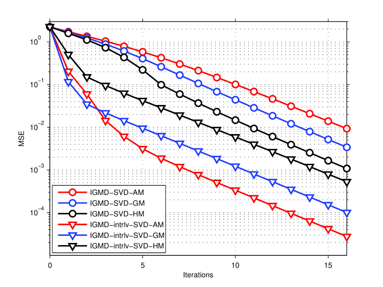
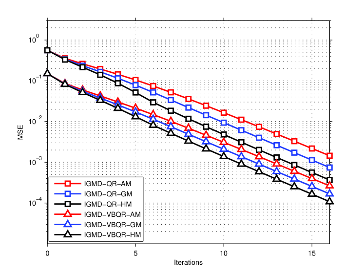
Fig. 1 and Fig. 2 show the mean-square-error (MSE) convergence behaviour of the diagonal elements of using SVD and QR as initializations, respectively. For SVD initialization, we propose an alternative interleaved-SVD (intrlv-SVD), defined as
| (43) |
where and to enable more efficient averaging in each stage. For QR initialization, the QR factorization with VBLAST ordering (VBQR) [21, 22] is also proposed to speed up convergence. As the diagonal elements of in VBQR generally has less spread than those in QR, VBQR initialization provides a smaller MSE when used in the initialization as shown in Fig. 2.
Due to the highly nonlinear nature of the corresponding mappings , , and , it is very difficult to analytically compare the convergence behaviour of the three IGMD constructions. Hence we resort to numerical simulations and leave the more challenging theoretical analysis to our future work. The simulation results in Fig. 1 and Fig. 2 show that the IGMD-HM has the fastest convergence rate, followed by the IGMD-GM, and the IGMD-AM when QR, VBQR, and SVD are used as initialization. On the other hand, when intrlv-SVD are used, the IGMD-AM has the fastest convergence rate, followed by the IGMD-GM, and finally the IGMD-HM.
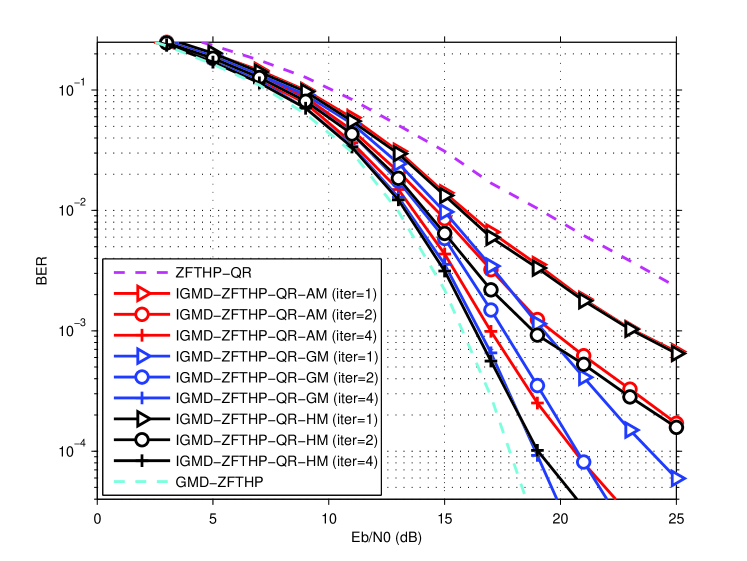
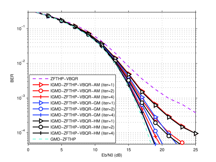
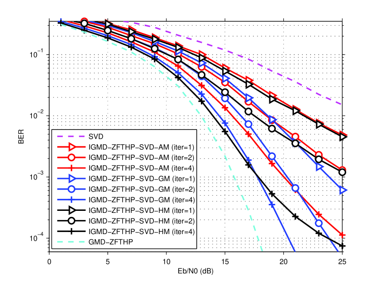
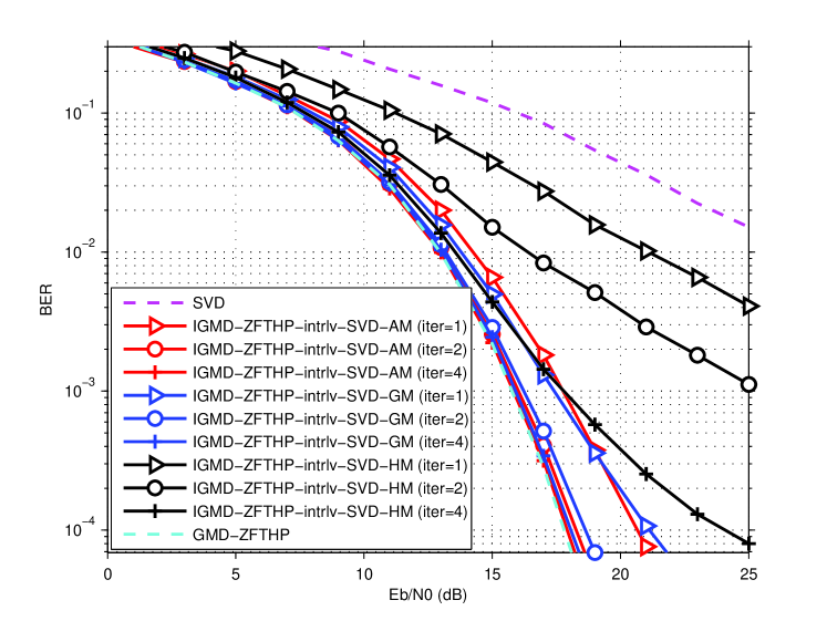
In the second simulation setting, we investigate the convergence behaviour of the proposed IGMD on the error rate performance of a GMD-based MIMO system. A GMD-based zero-forcing Tomlinson-Harashima precoded (ZFTHP) MIMO system [4] using -quadrature amplitude modulation is simulated. Fig. 3 and Fig. 4 show the error rate of the proposed IGMD using QR and VBQR, respectively. By comparing the BER of ZFTHP-QR in Fig. 3 and ZFTHP-VBQR in Fig. 4, it is clear that the VBQR provides a better initialization for the proposed IGMD, and results in faster convergence. At the st iteration, the error rate performance of IGMD-AM and IGMD-HM appears to be similar. However, for iteration number greater than , the IGMD-GM and IGMD-HM both outperform the IGMD-AM and perform very close to the optimal GMD after iterations.
Fig. 5 and Fig. 6 show the error rate of the proposed IGMD using regular SVD and interleaved SVD, respectively. In medium to low SNR region, the IGMD-HM shows comparable or even better performance than the IGMD-GM, while for sufficiently high SNR, the IGMD-GM performs the best, followed by the IGMD-HM, and the IGMD-AM. On the contrary, the proposed IGMD using interleaved SVD as initialization shows very different convergence behaviour. The IGMD-HM with interleaved SVD performs much worse compared to the IGMD-AM and IGMD-GM. For most SNR region of practical interests in this setting, the IGMD-AM is comparable to the IGMD-GM for iteration number greater than . From Fig. 4 and Fig 6, it is observed that the proposed IGMD-intrlv-SVD-GM and IGMD-intrlv-SVD-AM achieve even better error rate than the IGMD-VBQR-GM and IGMD-VBQR-HM after iterations.
V Conclusion
An iterative geometric mean decomposition algorithm for MIMO communications is proposed. The proposed algorithm has a regular structure and can be easily adapted to accommodate problems of different dimensions. Through iteratively updating the constituents matrices, the algorithm is able to converge to the true GMD without performing the th root computation. The convergence of the algorithm under certain sufficient condition is proved analytically and verified through computer simulations.
Acknowledgment
The authors would like to thank Prof. Chiu-Chu Melissa Liu for the helpful discussion.
References
- [1] E. Telatar, “Capacity of multi-antenna gaussian channels,” Europ. Trans. Telecommu., vol. 10, pp. 585–595, Nov.-Dec. 1999.
- [2] G. J. Foschini, “Layered space-time architecture for wireless communication in a fading environment when using multiple antennas,” Bell Labs Tech. Journal, vol. 1, pp. 41–59, 1996.
- [3] G. G. Raleigh and J. M. Cioffi, “Spatio-temporal coding for wireless communication,” IEEE Trans. Commun., vol. 46, no. 3, pp. 357–366, Mar. 1998.
- [4] Y. Jiang, J. Li, and W. Hager, “Joint transceiver design for mimo communications using geometric mean decomposition,” IEEE Trans. Signal Process., vol. 53, no. 10, pp. 3791–3803, Oct. 2005.
- [5] Y. Jiang, J. Li, and W. W. Hager, “Uniform channel decomposition for MIMO communications,” IEEE Trans. Signal Process., vol. 53, pp. 4283–4294, Nov. 2005.
- [6] J.-K. Zhang, A. Kavčić, and K. M. Wong, “Equal-diagonal QR decomposition and its application to precoder design for successive-cancellation detection,” IEEE Trans. Inf. Theory, vol. 51, no. 1, pp. 154–172, Jan. 2005.
- [7] Y. Jiang, W. Hager, and J. Li, “The geometric mean decomposition,” Linear Algebra and its Applications, vol. 396, pp. 373–384, Feb. 2005.
- [8] S. Lin, W. W. L. Ho, and Y.-C. Liang, “Block diagonal geometric mean decomposition (BD-GMD) for MIMO broadcast channels,” IEEE Trans. Wireless Commun., vol. 7, no. 7, p. 2778, Jul. 2008.
- [9] F. Liu, L. Jiang, and C. He, “Advanced joint transceiver design for block diagonal geometric mean decomposition based multiuser MIMO system,” IEEE Transactions Vehicular Technology, vol. 59, pp. 692–703, Feb. 2010.
- [10] C.-C. Weng and P. P. Vaidyanathan, “Block diagonal GMD for zero-padded MIMO frequency selective channels,” IEEE Trans. Signal Process., vol. 59, no. 2, pp. 713–727, Feb. 2011.
- [11] C.-H. Liu and P. P. Vaidyanathan, “Generalized geometric mean decomposition and DFE transceiver design—part i: design and complexity,” IEEE Trans. Signal Process., vol. 60, no. 6, pp. 3112–3123, Jun. 2012.
- [12] ——, “Generalized geometric mean decomposition and DFE transceiver design—part ii: performance analysis,” IEEE Trans. Signal Process., vol. 60, no. 6, pp. 3124–3133, Jun. 2012.
- [13] W. C. Kan and G. E. Sobelman, “MIMO transceiver design based on a modified geometric mean decomposition,” in Proc. IEEE Int. Symp. Circuits Syst., New Orleans, LA, May 2007, pp. 677–680.
- [14] W.-D. Chen and Y.-T. Hwang, “A constant throughput geometric mean decomposition scheme design for wireless MIMO precoding,” IEEE Trans. Veh. Tech., vol. 62, no. 5, pp. 2080–2090, Jun. 2013.
- [15] P. K. Meher, J. Vallas, T.-B. Juang, K. Sridharan, and K. Maharatna, “ years of CORDIC: algorithms, architectures, and applications,” IEEE Trans. Circuits Syst. I, Reg. Papers, vol. 56, pp. 1893–1907, Sep. 2009.
- [16] K. E. Atkinson, An introduction to numerical analysis, 2nd ed. New York: Wiley, 1989.
- [17] G. H. Golub and C. F. V. Loan, Matrix computations, 3rd ed. Baltimore and London: The Johns Hopkins University Press, 1996.
- [18] H. Weyl, “Inequalities between two kinds of eigenvalues of a linear transformation,” Proc. Nat. Acad. Sci. U.S.A., vol. 35, pp. 408–411, 1949.
- [19] A. W. Marshall and I. Olkin, Inequalities: Theory of Majorization and its Applications. New York: Academic, 1991.
- [20] W. Rudin, Principles of Mathematical Analysis, 3rd ed. McGraw-Hill, 1976.
- [21] P. W. Wolniansky, G. J. Foschini, G. D. Golden, and R. A. Valenzuela, “V-BLAST: an architecture for realizing very high data rates over the rich-scattering wireless channel,” in Proc. URSI International Symposium on Signals Systems and Electronics, 1998, pp. 295–300.
- [22] G. D. Golden, G. J. Foschini, R. A. Valenzuela, and P. W. Wolniansky, “Detection algorithm and initial laboratory results using V-BLAST space time communications architecture,” Electronic Letters, vol. 35, pp. 14–16, Jan. 1999.
