Gene-proximity models for Genome-Wide Association Studies

Abstract

Motivated by the important problem of detecting association between genetic markers and binary traits in genome-wide association studies, we present a novel Bayesian model that establishes a hierarchy between markers and genes by defining weights according to gene lengths and distances from genes to markers. The proposed hierarchical model uses these weights to define unique prior probabilities of association for markers based on their proximities to genes that are believed to be relevant to the trait of interest. We use an expectation-maximization algorithm in a filtering step to first reduce the dimensionality of the data and then sample from the posterior distribution of the model parameters to estimate posterior probabilities of association for the markers. We offer practical and meaningful guidelines for the selection of the model tuning parameters and propose a pipeline that exploits a singular value decomposition on the raw data to make our model run efficiently on large data sets. We demonstrate the performance of the model in simulation studies and conclude by discussing the results of a case study using a real-world dataset provided by the Wellcome Trust Case Control Consortium.

, , , t3Supported in part by JSPS KAKENHI grant 24300056. and t4Supported in part by NSF grant DMS-1107067.

1 Introduction

A genome-wide association study (GWAS) aims to determine the subset of genetic markers that is most relevant to a particular trait of interest. From a statistical perspective, this task is usually framed as a regression problem where the response variables are measurements of either qualitative traits, e.g., a binary value indicating the presence or absence of a disease, or quantitative traits, e.g., a person’s blood pressure, and the explanatory variables are the number of reference alleles present at each marker, or single nucleotide polymorphism (SNP), as well as other covariates of interest such as age or smoking status. Many linear models (Balding, 2006; Stephens and Balding, 2009) have been developed to detect associations between SNPs and traits, but they generally suffer from the “large $p$, small $n$” problem where the ratio of the number of predictors, $p$, to the sample size, $n$, is on the order of hundreds to thousands (West, 2003). Moreover, other issues such as collinearity in the covariates due to linkage disequilibrium [LD, (Pritchard and Przeworski, 2001)], rare variants, and population stratification result in inefficient estimation of model parameters and a loss in statistical power to detect significant associations (Wang et al., 2005).

A common strategy to overcome the large-$p$-small-$n$ problem in GWAS is to forgo analyzing the SNPs jointly and to model instead them independently. Although successful GWAS have employed this strategy (Burton et al., 2007), multiple hypothesis testing leads to an increase in the Type I error and the necessary correction for this may lead to an overly conservative threshold for statistical significance. Strategies such as grouping SNPs based on proximities to genes (Wu et al., 2010) or moving windows (Wu et al., 2011) have been proposed to allow for an increase in power by modeling SNPs jointly, but there is no universal agreement on how to define such windows or groupings. Similarly, other strategies include replacing a group of highly correlated SNPs with only one of its members (Ioannidis et al., 2009), and removing or collapsing rare variants within a window into a score statistic (Bansal et al., 2010), but again there is no agreement on how to choose which SNPs to retain or group. Recent approaches aim at gaining more power by pooling information across studies through meta-analysis (Evangelou and Ioannidis, 2013).

Although significant progress has been made on GWAS since 2000, it is still a relevant and challenging problem with goals such as modeling interactions between SNPs, genes, and environment effects that await beyond the obstacles already mentioned (Heard et al., 2010). In order to move towards a unifying framework for GWAS that allows for the large-$p$-small-$n$ problem and the SNP-specific issues to be addressed simultaneously in a principled manner, we propose a novel hierarchical Bayesian model that exploits spatial relationships on the genome to define SNP-specific prior distributions on regression parameters. More specifically, in our proposed setting we model markers jointly, but we explore a variable selection approach that uses marker proximity to relevant genomic regions, such as genes, to help identify associated SNPs. Our contributions are:

1. We focus on binary traits which are arguably more common to GWAS, e.g., case control studies, but more difficult to model due to lack of conjugacy. To circumvent the need for a Metropolis-Hastings step when sampling from the posterior distribution on model parameters, we use a recently proposed data augmentation strategy for logistic regression based on latent Pólya-Gamma random variables (Polson et al., 2013).

2. We perform variable selection by adopting a spike-and-slab prior (George and McCulloch, 1993; Ishwaran and Rao, 2005) and propose a principled way to control the separation between the spike and slab components using a Bayesian false discovery rate similar to (Whittemore, 2007).

3. We use a novel weighting scheme to establish a relationship between SNPs and genomic regions and allow for SNP-specific prior distributions on the model parameters such that the prior probability of association for each SNP is a function of its location on the chromosome relative to neighboring regions. Moreover, we allow for the “relevance” of a genomic region to contribute to the effect it has on its neighboring SNPs and consider “relevance” values calculated based on previous GWAS results in the literature, e.g. see (MalaCards, 2014).

4. Before sampling from the posterior space using Gibbs sampling, we use an expectation-maximization [EM, (Dempster et al., 1977)] algorithm in a filtering step to reduce the number of candidate markers in a manner akin to distilled sensing (Haupt et al., 2011). By investigating the update equations for the EM algorithm, we suggest meaningful values to tune the hyperprior parameters of our model and illustrate the induced relationship between SNPs and genomic regions.

5. We derive a more flexible centroid estimator (Carvalho and Lawrence, 2008) for SNP associations that is parameterized by a sensitivity-specificity trade-off. We discuss the relation between this parameter and the prior specification when obtaining estimates of model parameters.

We start by describing previous work and stating our contributions in Section 2. In Section 3 we define our Spatial Boost model and the novel relationship between SNPs and genes. In Section 4 we describe how to fit the model using a combination of a filtering step that exploits an EM filtering step and Gibbs sampling. We provide guidelines for the selection of model tuning parameters in Section 5. We then illustrate the performance of the model on simulated data using real SNPs in Section 6 and apply the model to a real-world GWAS data set provided by the Wellcome Trust Case Control Consortium (WTCCC) in Section 7. Finally, we conclude with a discussion on future extensions to this work in Section 8.

2 Previous and Related Work

A common solution to large-$p$-small-$n$ problems is to use penalized regression models such as ridge regression (Hoerl and Kennard, 1970), LASSO (Tibshirani, 1996), or elastic net (Zou and Hastie, 2005). These solutions can be shown to be equivalent, from a Bayesian perspective, to maximum a posteriori (MAP) estimators under appropriate prior specifications. For instance, for LASSO, the $L_{1}$ penalty can be translated into a Laplace prior. However, since LASSO produces biased estimates of the model parameters and tends to select only one parameter in a group of correlated parameters (Zou and Hastie, 2005), it is not suitable for GWAS.

Techniques like group LASSO, fused LASSO (Tibshirani and Saunders, 2005), or sparse group LASSO (Friedman et al., 2010) further attempt to account for the structure of genes and markers or linkage disequilibrium by assigning SNPs to groups based on criteria such as gene membership and then placing additional penalties on the $L_{1}$ norm of the vector of coefficients for each group, or on the $L_{1}$ norm of the difference in coefficients of consecutive SNPs. However, it is difficult to define gene membership universally since genes have varying lengths and may overlap with each other; moreover, the penalty on the $L_{1}$ norm of the difference in consecutive SNPs neglects any information contained in the genomic distance between them.

It may be possible to develop additional, effective penalty terms within models, such as $L_{1}$ and $L_{2}$, to address the issues present in GWAS data in a penalized regression framework, but because genotypes are more correlated for markers that are close in genomic space due to linkage disequilibrium, the most effective penalties would need to capture the relevance of a particular SNP as a function of its location on the genome. Moreover, since it is typically easier to study the biological function of genes, we are particularly interested in SNPs that lie close to genes (Jorgenson and Witte, 2006); as a result, the most desirable penalties would likely be SNP-specific. We accomplish this by exploiting biological knowledge about the structure of the genome to set SNP-specific prior distributions on the model parameters in a hierarchical Bayesian model.

Researchers have considered hierarchical Bayesian models for variable selection in GWAS and other large scale problems (e.g. (Guan and Stephens, 2011; Zhou et al., 2013)). Some recent models exploit Bayesian methods in particular to allow for data-driven SNP-specific prior distributions (Habier et al., 2011) which depend on a random variable that describes the proportion of SNPs to be selected. These approaches have adopted a continuous spike-and-slab prior distribution (George and McCulloch, 1993; Ishwaran and Rao, 2005) on the model parameters, set an inverse-gamma prior distribution on the variance of the spike component of the prior, and control the difference in the variance of the spike and slab components of the prior using a tuning parameter.

To incorporate external information in a hierarchical Bayesian model, researchers analyzing a different kind of data, gene expression levels, have recently considered relating a linear combination of a set of predictor-level covariates that quantify the relationships between the genes to their prior probabilities of association through a probit link function (Peng et al., 2013). This formulation leads to a second-stage probit regression on the probability that any gene is associated with a trait of interest using a set of predictor-level covariates that could be, for instance, indicator variables of molecular pathway membership. In our model, we propose a special case of this formulation tailored for GWAS data where: (i) we use the logit link instead of the probit link, (ii) the predictor-level covariates are spatial weights that quantify a SNP’s position on the genome relative to neighboring genes, and (iii) the coefficients of each of the predictor-level covariates are numerical scores that quantify the relevance of a particular gene to the trait of interest.

Fitting a penalized model to a large data set (e.g. $p\geq 100,\!000$) is computationally intense and thus so is the process of selecting an optimal value for any tuning parameters. Side-stepping this problem, some researchers have had success in applying a suite of penalty terms (e.g. LASSO, Adaptive LASSO, NEG, MCP, LOG) to a pre-screened subset of markers (Hoffman et al., 2013) and investigating the concordance of significant markers across each of the final models. Although a pre-screening of markers from a marginal regression would ideally retain almost all of the relevant variables, penalized models such as LASSO could likely be improved by using a larger number of SNPs than those which pass an initial screening step (e.g. a genome-wide significance threshold) (Kooperberg et al., 2010).

3 Spatial Boost Model

We perform Bayesian variable selection by analyzing binary traits and using the structure of the genome to dynamically define the prior probabilities of association for the SNPs. Our data are the binary responses $\mathbf{y}\in{\{0,1\}}^{n}$ for $n$ individuals and genotypes ${\mathbf{x}}_{i}\in{\{0,1,2\}}^{p}$ for $p$ markers per individual, where $x_{ij}$ codes the number of minor alleles in the $i$-th individual for the $j$-th marker. For the likelihood of the data, we consider the logistic regression:

$$y_{i}{\,|\,}\mathbf{x}_{i},\beta\stackrel{{\scriptstyle\text{\tiny ind}}}{{\sim}}\text{\sf Bern}\big{(}{\rm logit}^{-1}(\beta_{0}+\mathbf{x}_{i}^{\top}\beta)\big{)},\quad\text{for~{}}i=1,\ldots,n.$$ (1)

We note that GWA studies are usually retrospective, i.e. cases and controls are selected irrespectively of their history or genotypes; however, as McCullagh and Nelder (1989) point out, coefficient estimates for $\beta$ are not affected by the sampling design under a logistic regression. Thus, from now on, to alleviate the notation we extend $\mathbf{x}_{i}$ to incorporate the intercept, $\mathbf{x}_{i}=(x_{i0}=1,x_{i1},\ldots,x_{ip})$, and also set $\beta=(\beta_{0},\beta_{1},\ldots,\beta_{p})$.

We use latent variables $\theta\in{\{0,1\}}^{p}$ and a continuous spike-and-slab prior distribution for the model parameters with the positive constant $\kappa>1$ denoting the separation between the variance of the spike and the slab components:

$$\beta_{j}{\,|\,}\theta_{j},\sigma^{2}\stackrel{{\scriptstyle\text{\tiny ind}}}{{\sim}}\text{\sf N}\big{(}0,\sigma^{2}[\theta_{j}\kappa+(1-\theta_{j})]\big{)},\quad\text{for~{}}j=1,\ldots,p.$$ (2)

For the intercept, we set $\beta_{0}\sim N(0,\sigma^{2}\kappa)$ or, equivalently, we define $\theta_{0}=1$ and include $j=0$ in (2). In the original spike-and-slab prior distribution, the slab component is a normal distribution centered at zero with a large variance or even a diffuse uniform distribution and the spike component is a degenerate distribution at zero (Mitchell and Beauchamp, 1988). This setup results in exact variable selection through the use of the $\theta_{j}$’s, since $\theta_{j}=0$ would imply that the $j$-th SNP’s coefficient is exactly equal to zero. Here we use the continuous version of the spike-and-slab distribution (George and McCulloch, 1993; Ishwaran and Rao, 2005) that became more popular by avoiding the spike discontinuities at zero and thus allowing for a relaxed form of variable selection that lends itself easily to an EM algorithm (see Section 4.1).

For the variance $\sigma^{2}$ of the spike component in (2) we adopt an inverse Gamma prior distribution, $\sigma^{2}\sim\text{\sf IG}(\nu,\lambda)$. We expect $\sigma^{2}$ to be reasonably small with high probability in order to enforce the desired regularization that distinguishes selected markers from non-associated markers. Thus, we recommend choosing $\nu$ and $\lambda$ so that the prior expected value of $\sigma^{2}$ is small.

In the prior distribution for $\theta_{j}$, we incorporate information from relevant genomic regions. The most common instance of such regions are genes, and so we focus on these regions in what follows. Thus, given a list of $G$ genes with gene relevances (see Section 3.2 for some choices of definitions), $\mathbf{r}=[r_{1},r_{2},\ldots,r_{G}]$, and weights, $\mathbf{w}_{j}(\phi)=[w_{j,1},w_{j,2},\ldots,w_{j,G}]$, the prior on $\theta_{j}$ is

$$\theta_{j}\stackrel{{\scriptstyle\text{\tiny ind}}}{{\sim}}\text{\sf Bern}\big{(}{\rm logit}^{-1}(\xi_{0}+\xi_{1}{\mathbf{w}_{j}(\phi)}^{\top}\mathbf{r})\big{)},\quad\text{for~{}}j=1,\ldots,p.$$ (3)

The weights $\mathbf{w}_{j}$ are defined using the structure of the SNPs and genes and aim to account for gene lengths and their proximity to markers as a function of a spatial parameter $\phi$, as we see in more detail next.

Figure 1: Gene weight example: for the $j$-th SNP at position $s_{j}=1,\!000$ and two surrounding genes $a$ and $b$ spanning $(980,995)$ and $(1020,1030)$ we obtain, if setting $\phi=10$, weights of $w_{j,a}=0.29$ and $w_{j,b}=0.02$, respectively.

3.1 Gene Weights

To control how much a gene can contribute to the prior probability of association for a SNP based on the gene’s length and distance to that SNP we introduce a range parameter $\phi>0$. Consider a gene $g$ that spans genomic positions $g_{l}$ to $g_{r}$, and the $j$-th marker at genomic position $s_{j}$; the gene weight $w_{j,g}$ is then

$$w_{j,g}=\int_{g_{l}}^{g_{r}}\dfrac{1}{\sqrt{2\pi\phi^{2}}}\text{exp}\Bigg{\{}-\dfrac{{(x-s_{j})}^{2}}{2\phi^{2}}\Bigg{\}}\,\mathrm{d}x.$$

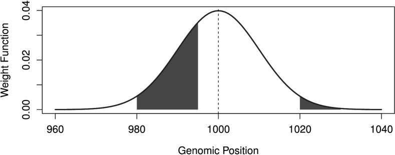
Generating gene weights for a particular SNP is equivalent to centering a Gaussian curve at that SNP’s position on the genome with standard deviation equal to $\phi$ and computing the area under that curve between the start and end points of each gene. Figure 1 shows an example. As $\phi\to 0$, the weight that each gene contributes to a particular SNP becomes an indicator function for whether or not it covers that SNP; as $\phi\to\infty$, the weights decay to zero. Intermediate values of $\phi$ allow then for a variety of weights in $[0,1]$ that encode spatial information about gene lengths and gene proximities to SNPs. In Section 5.1 we discuss a method to select $\phi$.

According to (3), it might be possible for multiple, possibly overlapping, genes that are proximal to SNP $j$ to boost $\theta_{j}$. To avoid this effect, we take two precautions. First, we break genes into non-overlapping genomic blocks and define the relevance of a block as the mean gene relevance of all genes that cover the block. Second, we normalize the gene weight contributions to $\theta_{j}$ in (3), ${\mathbf{w}_{j}(\phi)}^{\top}\mathbf{r}$, such that $\max_{j}{\mathbf{w}_{j}(\phi)}^{\top}\mathbf{r}=1$. This way, it is possible to compare estimates of $\xi_{1}$ across different gene weight and relevance schemes.

3.2 Gene Relevances

We allow for the further strengthening or diminishing of particular gene weights using gene relevances $\mathbf{r}$. If we set $\mathbf{r}=\mathbf{1}_{G}$ and allow for all genes to be uniformly relevant, then we have a “non-informative” case. Alternatively, if we have some reason to believe that certain genes are more relevant to a particular trait than others, for instance on the basis of previous research or prior knowledge from an expert, then we can encode these beliefs through $\mathbf{r}$. In particular, we recommend using either text-mining techniques, e.g. (Al-Mubaid and Singh, 2010), to quantify the relevance of a gene to a particular disease based on citation counts in the literature, or relevance scores compiled from search hits and citation linking the trait of interest to genes, e.g. (MalaCards, 2014).

4 Model Fitting and Inference

The ultimate goal of our model is to perform inference on the posterior probability of association for SNPs. However, these probabilities are not available in closed form, and so we must resort to Markov chain Monte Carlo techniques such as Gibbs sampling to draw samples from the posterior distributions of the model parameters and use them to estimate ${\mathbb{P}}(\theta_{j}=1{\,|\,}\mathbf{y})$. Unfortunately, these techniques can be slow to iterate and converge, especially when the number of model parameters is large (Cowles and Carlin, 1996). Thus, to make our model more computationally feasible, we propose first filtering out markers to reduce the size of the original dataset in a strategy similar to distilled sensing (Haupt et al., 2011), and then applying a Gibbs sampler to only the remaining SNPs.

To this end, we design an EM algorithm based on the hierarchical model above that uses all SNP data simultaneously to quickly find an approximate mode of the posterior distribution on $\beta$ and $\sigma^{2}$ while regarding $\theta$ as missing data. Then, for the filtering step, we iterate between (1) removing a fraction of the markers that have the lowest conditional probabilities of association and (2) refitting using the EM procedure until the predictions of the filtered model degrade. In our analyses we filtered $25\%$ of the markers at each iteration to arrive at estimates $\beta^{*}$ and stopped if $\max_{i}|y_{i}-{\rm logit}^{-1}(\mathbf{x}_{i}^{\top}\beta^{*})|>0.5$. Next, we discuss the EM algorithm and the Gibbs sampler, and offer guidelines for selecting the other parameters of the model in Section 5.

4.1 EM algorithm

We treat $\theta$ as a latent parameter and build an EM algorithm accordingly. If $\ell(\mathbf{y},\theta,\beta,\sigma^{2})=\log{\mathbb{P}}(\mathbf{y},\theta,\beta,\sigma^{2})$ then for the M-steps on $\beta$ and $\sigma^{2}$ we maximize the expected log joint $Q(\beta,\sigma^{2};\beta^{(t)},{(\sigma^{2})}^{(t)})={\mathbb{E}}_{\theta{\,|\,}\mathbf{y},X;\beta^{(t)},{(\sigma^{2})}^{(t)}}[\ell(\mathbf{y},\theta,\beta,\sigma^{2})]$. The log joint distribution $\ell$, up to a normalizing constant, is

$$\ell(\mathbf{y},\theta,\beta,\sigma^{2})=\sum_{i=1}^{n}y_{i}\mathbf{x}_{i}^{\top}\beta-\log(1+\exp\{\mathbf{x}_{i}^{\top}\beta\})\\ -\dfrac{p+1}{2}\log\sigma^{2}-\dfrac{1}{2\sigma^{2}}\sum_{j=0}^{p}\beta_{j}^{2}\Bigg{(}\dfrac{\theta_{j}}{\kappa}+1-\theta_{j}\Bigg{)}-(\nu+1)\log\sigma^{2}-\dfrac{\lambda}{\sigma^{2}},$$ (4)

and so, at the $t$-th iteration of the procedure, for the E-step we just need $\langle\theta_{j}\rangle^{(t)}\doteq{\mathbb{E}}_{\theta{\,|\,}\mathbf{y};\beta^{(t)},{(\sigma^{2})}^{(t)}}[\theta_{j}]$. But since

$$\langle\theta_{j}\rangle={\mathbb{P}}(\theta_{j}=1{\,|\,}\mathbf{y},\beta,\sigma^{2})=\dfrac{{\mathbb{P}}(\theta_{j}=1,\beta_{j}{\,|\,}\sigma^{2})}{{\mathbb{P}}(\theta_{j}=0,\beta_{j}{\,|\,}\sigma^{2})+{\mathbb{P}}(\theta_{j}=1,\beta_{j}{\,|\,}\sigma^{2})},$$

then

$${\rm logit}\langle\theta_{j}\rangle=\log\dfrac{{\mathbb{P}}(\theta_{j}=1,\beta_{j}{\,|\,}\sigma^{2})}{{\mathbb{P}}(\theta_{j}=0,\beta_{j}{\,|\,}\sigma^{2})}=-\dfrac{1}{2}\log\kappa-\dfrac{\beta_{j}^{2}}{2\sigma^{2}}\Bigg{(}\dfrac{1}{\kappa}-1\Bigg{)}+\xi_{0}+\xi_{1}\mathbf{w}_{j}^{\top}\mathbf{r}$$ (5)

for $j=1,\ldots,p$ and $\langle\theta_{0}\rangle\doteq 1$.

To update $\beta$ and $\sigma^{2}$ we employ conditional maximization steps (Meng and Rubin, 1993), similar to cyclic gradient descent. From (4) we see that the update for $\sigma^{2}$ follows immediately from the mode of an inverse gamma distribution conditional on $\beta^{(t)}$:

$${(\sigma^{2})}^{(t+1)}=\frac{\dfrac{1}{2}\displaystyle\sum_{j=0}^{p}{(\beta_{j}^{(t)})}^{2}\Bigg{(}\dfrac{\langle\theta_{j}\rangle^{(t)}}{\kappa}+1-\langle\theta_{j}\rangle^{(t)}\Bigg{)}+\lambda}{\dfrac{p+1}{2}+\nu+1}.$$ (6)

The terms in (4) that depend on $\beta$ come from the log likelihood of $\mathbf{y}$ and from the expected prior on $\beta$, $\beta\sim N(0,\Sigma^{(t)})$, where

$$\Sigma^{(t)}=\text{Diag}\Bigg{(}\dfrac{\sigma^{2}}{\langle\theta_{j}\rangle^{(t)}/\kappa+1-\langle\theta_{j}\rangle^{(t)}}\Bigg{)}.$$

Since updating $\beta$ is equivalent here to fitting a ridge regularized logistic regression, we exploit the usual iteratively reweighted least squares (IRLS) algorithm (MacCullagh and Nelder, 1989). Setting $\mu^{(t)}$ as the vector of expected responses with $\mu^{(t)}_{i}={\rm logit}^{-1}(\mathbf{x}_{i}^{\top}\beta^{(t)})$ and $W^{(t)}=\text{Diag}(\mu^{(t)}_{i}(1-\mu^{(t)}_{i}))$ as the variance weights, the update for $\beta$ is then

$$\beta^{(t+1)}={(X^{\top}W^{(t)}X+{(\Sigma^{(t)})}^{-1})}^{-1}\big{(}X^{\top}W^{(t)}X\beta^{(t)}+X^{\top}(\mathbf{y}-\mu^{(t)})\big{)},$$ (7)

where we substitute ${(\sigma^{2})}^{(t)}$ for $\sigma^{2}$ in the definition of $\Sigma^{(t)}$.

Rank truncation of design matrix

Computing and storing the inverse of the $(p+1)$-by-$(p+1)$ matrix $X^{\top}W^{(t)}X+{(\Sigma^{(t)})}^{-1}$ in (7) is expensive since $p$ is large. To alleviate this problem, we replace $X$ with a rank truncated version based on its singular value decomposition $X=UDV^{\top}$. More specifically, we take the top $l$ singular values and their respective left and right singular vectors, and so, if $D=\text{Diag}(d_{i})$ and $\mathbf{u}_{i}$ and $\mathbf{v}_{i}$ are the $i$-th left and right singular vectors respectively,

$$X=UDV^{\top}=\sum_{i=1}^{n}d_{i}\mathbf{u}_{i}\mathbf{v}_{i}^{\top}\approx\sum_{i=1}^{l}d_{i}\mathbf{u}_{i}\mathbf{v}_{i}^{\top}=U_{(l)}D_{(l)}V_{(l)}^{\top},$$

where $D_{(l)}$ is the $l$-th order diagonal matrix with the top $l$ singular values and $U_{(l)}$ ($n$-by-$l$) and $V_{(l)}$ ($(p+1)$-by-$l$) contain the respective left and right singular vectors. We select $l$ by controlling the mean squared error: $l$ should be large enough such that $\|X-U_{(l)}D_{(l)}V_{(l)}^{\top}\|_{F}/(n(p+1))<0.01$.

Since $X^{\top}W^{(t)}X\approx V_{(l)}D_{(l)}U_{(l)}^{\top}W^{(t)}U_{(l)}D_{(l)}V_{(l)}^{\top}$, we profit from the rank truncation by defining the (upper) Cholesky factor $C_{w}$ of $D_{(l)}U_{(l)}^{\top}W^{(t)}U_{(l)}D_{(l)}$ and $S=C_{w}V_{(l)}^{\top}$ so that

$$\begin{split}{(X^{\top}W^{(t)}X+{(\Sigma^{(t)})}^{-1})}^{-1}&\approx{(S^{\top}S+{(\Sigma^{(t)})}^{-1})}^{-1}\\ &=\Sigma^{(t)}-\Sigma^{(t)}S^{\top}{(I_{l}+S\Sigma^{(t)}S^{\top})}^{-1}S\Sigma^{(t)}\end{split}$$ (8)

by the Kailath variant of the Woodbury identity (Petersen and Pedersen, 2008). Now we just need to store and compute the inverse of the $l$-th order square matrix $I_{l}+S\Sigma^{(t)}S^{\top}$ to obtain the updated $\beta^{(t+1)}$ in (7).

4.2 Gibbs sampler

After obtaining results from the EM filtering procedure, we proceed to analyze the filtered dataset by sampling from the joint posterior ${\mathbb{P}}(\theta,\beta,\sigma^{2}{\,|\,}\mathbf{y})$ using Gibbs sampling. We iterate sampling from the conditional distributions

$$[\sigma^{2}{\,|\,}\theta,\beta,\mathbf{y}],\quad[\theta{\,|\,}\beta,\sigma^{2},\mathbf{y}],\quad\text{and}\quad[\beta{\,|\,}\theta,\sigma^{2},\mathbf{y}]$$

until assessed convergence.

We start by taking advantage of the conjugate prior for $\sigma^{2}$ and draw each new sample from

$$\sigma^{2}{\,|\,}\theta,\beta,\mathbf{y}\sim\text{\sf IG}\Bigg{(}\nu+\dfrac{p+1}{2},\,\lambda+\dfrac{1}{2}\sum_{j=0}^{p}\beta_{j}^{2}\Big{(}\dfrac{\theta_{j}}{\kappa}+1-\theta_{j}\Big{)}\Bigg{)}.$$

Sampling $\theta$ is also straightforward: since the $\theta_{j}$ are independent given $\beta_{j}$,

$$\theta_{j}{\,|\,}\beta,\sigma^{2},\mathbf{y}\stackrel{{\scriptstyle\text{\tiny ind}}}{{\sim}}\text{\sf Bern}(\langle\theta_{j}\rangle),\quad\text{for~{}}j=1,\ldots,p,$$

with $\langle\theta_{j}\rangle$ as in (5). Sampling $\beta$, however, is more challenging since there is no closed-form distribution based on a logistic regression, but we use a data augmentation scheme proposed by Polson et al. (2013). This method has been noted to perform well when the model has a complex prior structure and the data have a group structure and so we believe it is appropriate for the Spatial Boost model.

Thus, to sample $\beta$ conditional on $\theta$, $\sigma^{2}$, and $\mathbf{y}$ we first sample latent variables $\omega$ from a Pólya-Gamma distribution,

$$\omega_{i}{\,|\,}\beta\sim\text{\sf PG}(1,\mathbf{x}_{i}^{\top}\beta),\quad i=1,\ldots,n,$$

and then, setting $\Omega=\text{Diag}(\omega_{i})$, $\Sigma=\text{Diag}(\sigma^{2}(\theta_{j}\kappa+1-\theta_{j}))$, and $V_{\beta}=X^{\top}\Omega X+\Sigma^{-1}$, sample

$$\beta{\,|\,}\omega,\theta,\sigma^{2},\mathbf{y}\sim N(V_{\beta}^{-1}X^{\top}(\mathbf{y}-0.5\cdot\mathbf{1}_{n}),\,V_{\beta}^{-1}).$$

We note that the same rank truncation used in the EM algorithm from the previous section works here, and we gain more computational efficiency by using an identity similar to (8) when computing and storing $V_{\beta}^{-1}$.

4.3 Centroid estimation

To conduct inference on $\theta$ we follow statistical decision theory (Berger, 1985) and define an estimator based on a generalized Hamming loss function $H(\theta,\widetilde{\theta})=\sum_{j=1}^{p}h(\theta_{j},\widetilde{\theta}_{j})$,

$$\widehat{\theta}_{C}=\mathop{\rm arg\,min}\limits_{\widetilde{\theta}\in{\{0,1\}}^{p}}{\mathbb{E}}_{\theta{\,|\,}\mathbf{y}}\big{[}H(\theta,\widetilde{\theta})\big{]}=\mathop{\rm arg\,min}\limits_{\widetilde{\theta}\in{\{0,1\}}^{p}}{\mathbb{E}}_{\theta{\,|\,}\mathbf{y}}\Bigg{[}\sum_{j=1}^{p}h(\theta_{j},\widetilde{\theta}_{j})\Bigg{]}.$$ (9)

We assume that $h$ has symmetric error penalties, $h(0,1)=h(1,0)$ and that $h(1,0)>\max\{h(0,0),h(1,1)\}$, that is, the loss for a false positive or negative is higher than for a true positive and true negative. In this case, we can define a gain function $g$ by subtracting each entry in $h$ from $h(1,0)$ and dividing by $h(1,0)-h(0,0)$:

$$g(\theta_{j},\widetilde{\theta}_{j})=\begin{cases}1,&\theta_{j}=\widetilde{\theta}_{j}=0,\\ 0,&\theta_{j}\neq\widetilde{\theta}_{j},\\ \gamma\doteq\dfrac{h(1,0)-h(1,1)}{h(1,0)-h(0,0)},&\theta_{j}=\widetilde{\theta}_{j}=1.\\ \end{cases}$$

Gain $\gamma>0$ represents a sensitivity-specificity trade-off; if $h(0,0)=h(1,1)$, that is, if true positives and negatives have the same relevance, then $\gamma=1$.

Let us define the marginal posteriors $\pi_{j}\doteq{\mathbb{P}}(\theta_{j}=1{\,|\,}\mathbf{y})$. The above estimator is then equivalent to

$$\widehat{\theta}_{C}=\mathop{\rm arg\,max}\limits_{\widetilde{\theta}\in{\{0,1\}}^{p}}{\mathbb{E}}_{\theta{\,|\,}\mathbf{y}}\Bigg{[}\sum_{j=1}^{p}g(\theta_{j},\widetilde{\theta}_{j})\Bigg{]}\\ =\mathop{\rm arg\,max}\limits_{\widetilde{\theta}\in{\{0,1\}}^{p}}\sum_{j=1}^{p}(1-\widetilde{\theta}_{j})(1-\pi_{j})+\gamma\widetilde{\theta}_{j}\theta_{j}=\mathop{\rm arg\,max}\limits_{\widetilde{\theta}\in{\{0,1\}}^{p}}\sum_{j=1}^{p}\Bigg{(}\pi_{j}-\dfrac{1}{1+\gamma}\Bigg{)}\widetilde{\theta}_{j},$$

which can be obtained position-wise,

$${(\widehat{\theta}_{C})}_{j}=I\Bigg{(}\pi_{j}-\dfrac{1}{1+\gamma}\geq 0\Bigg{)}.$$ (10)

The estimator in (9) is known as the centroid estimator; in contrast to maximum a posteriori (MAP) estimators that simply identify the highest peak in a posterior distribution, centroid estimators can be shown to be closer to the mean than to a mode of the posterior space, and so offer a better summary of the posterior distribution (Carvalho and Lawrence, 2008). Related formulations of centroid estimation for binary spaces in (10) have been proposed in many bioinformatics applications in the context of maximum expected accuracy (Hamada and Asai, 2012). Moreover, if $\gamma=1$ then $\widehat{\theta}_{C}$ is simply a consensus estimator and coincides with the median probability model estimator of Barbieri and Berger (2004).

Finally, we note that the centroid estimator can be readily obtained from MCMC samples $\theta^{(1)},\ldots,\theta^{(N)}$ since we just need to estimate the marginal posterior probabilities $\widehat{\pi}_{j}=\sum_{s=1}^{N}\theta^{(s)}_{j}/N$ and apply them to (10).

5 Guidelines for Selecting Prior Parameters

Since genome-wide association is a large-$p$-small-$n$ problem, we rely on adequate priors to guide the inference and overcome ill-posedness. In this section we provide guidelines for selecting hyperpriors $\kappa$ in the slab variance of $\beta$, and $\phi$, $\xi_{0}$, and $\xi_{1}$ in the prior for $\theta$.

5.1 Selecting $\phi$

Biologically, some locations within a chromosome may be more prone to recombination events and consequently to relatively higher linkage disequilibrium. LD can be characterized as correlation in the genotypes, and since we analyze the entire genome, high correlation in markers within a chromosome often results in poor coefficient estimates for the logistic regression model in 1. To account for potentially varying spatial relationships across the genome, we exploit the typical correlation pattern in GWAS data sets to suggest a value for $\phi$ that properly encodes the spatial relationship between markers and genes in a particular region as a function of genomic distance. To this end, we propose the following procedure to select $\phi$:

1. Divide each chromosome into regions such that the distance between the SNPs in adjacent regions is at least the average length of a human gene, or $30,\!000$ base pairs (Technology Department Carnegie Library of Pittsburgh, 2002). The resulting regions will be, on average, at least a gene’s distance apart from each other and may possibly exhibit different patterns of correlation.

2. Merge together any adjacent regions that cover the same gene. Although the value of $\phi$ depends on each region, we want the meaning of the weights assigned from a particular gene to SNPs in the Spatial Boost model to be consistent across regions. As a practical example, by applying the first two steps of the pre-processing procedure on chromosome 1, we obtain 1,299 windows of varying sizes ranging from 1 to 300 markers.

3. Iterate over each region and select a value of $\phi$ that best fits the magnitude of the genotype correlation between any given pair of SNPs as a function of the distance between them. We propose using the normal curve given in the definition of the gene weights to first fit the magnitudes, and then using the mean squared error between the magnitudes in the sample correlation matrix of a region and the magnitudes in the fitted correlation matrix as a metric to decide the optimal value of $\phi$. In particular, given two SNPs located at positions $s_{i}$ and $s_{j}$, we relate the magnitude of the correlation between SNPs $i$ and $j$ to the area

   $$|\rho_{i,j}|(\phi)=2\Phi\Bigg{(}-\dfrac{|s_{i}-s_{j}|}{\phi}\Bigg{)},$$

   where $\Phi$ is the standard normal cumulative function.

   

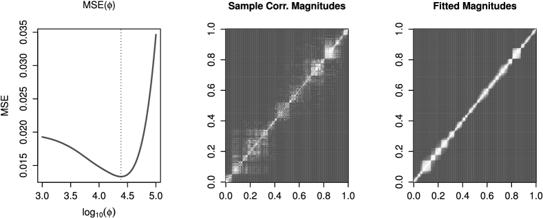
   Figure 2: Example of selection of $\phi$: when using the proposed values of $|\rho_{i,j}|$ to fit the sample correlation magnitudes, we obtain an optimal choice of $\phi=13,\!530$ for a random window.

   Figure 2 shows an example of application to chromosome 1 based on data from the case study discussed in Section 6. We note that the mean squared error criterion places more importance on fitting relatively larger magnitudes close to the diagonal of the image matrix, and so there is little harm in choosing a moderate value for $\phi$ that best fits the magnitudes of dense groups of correlated SNPs in close proximity.

5.2 Selecting $\xi_{0}$ and $\xi_{1}$

According to the centroid estimator in (10), the $j$-th SNP is identified as associated if $\pi_{j}\geq{(1+\gamma)}^{-1}$. Following a similar criterion, but with respect to the conditional posteriors, we have ${\mathbb{P}}(\theta_{j}=1{\,|\,}\mathbf{y},\beta,\sigma^{2})=\langle\theta_{j}\rangle\geq{(1+\gamma)}^{-1}$, and so, using (5),

$${\rm logit}\langle\theta_{j}\rangle=-\dfrac{1}{2}\log\kappa+\xi_{0}+\xi_{1}\mathbf{w}_{j}^{\top}\mathbf{r}+\dfrac{\beta_{j}^{2}}{2\sigma^{2}}\Bigg{(}1-\dfrac{1}{\kappa}\Bigg{)}\geq-\log\gamma.$$

After some rearrangements, we see that, in terms of $\beta_{j}$, this criterion is equivalent to $\beta_{j}^{2}\geq\sigma^{2}s_{j}^{2}$ with

$$s_{j}^{2}\doteq\dfrac{2\kappa}{\kappa-1}\Bigg{(}\dfrac{1}{2}\log\kappa-\xi_{0}-\xi_{1}\mathbf{w}_{j}^{\top}\mathbf{r}-\log\gamma\Bigg{)},$$ (11)

that is, we select the $j$-th marker if $\beta_{j}$ is more than $s_{j}$ “spike” standard deviations $\sigma$ away from zero.

This interpretation based on the EM formulation leads to a meaningful criterion for defining $\xi_{0}$ and $\xi_{1}$: we just require that $\min_{j=1,\ldots,p}s_{j}^{2}\geq s^{2}$, that is, that the smallest number of standard deviations is at least $s>0$. Since $\max_{j=1,\ldots,p}\mathbf{w}_{j}^{\top}\mathbf{r}=1$,

$$\min_{j=1,\ldots,p}s_{j}^{2}=\dfrac{2\kappa}{\kappa-1}\Bigg{(}\dfrac{1}{2}\log\kappa-\xi_{0}-\xi_{1}-\log\gamma\Bigg{)}\geq s^{2},$$

and so,

$$\xi_{1}\leq\dfrac{1}{2}\log\kappa-\xi_{0}-\log\gamma-\dfrac{s^{2}}{2}\Bigg{(}1-\dfrac{1}{\kappa}\Bigg{)}.$$ (12)

For a more stringent criterion, we can take the minimum over $\kappa$ in the right-hand side of (12) by setting $\kappa=s^{2}$. When setting $\xi_{1}$ it is also important to keep in mind that $\xi_{1}$ is the largest allowable gene boost, or better, increase in the log-odds of a marker being associated to the trait.

Since $\xi_{0}$ is related to the prior probability of a SNP being associated, we can take $\xi_{0}$ to be simply the logit of the fraction of markers that we expect to be associated a priori. However, for consistency, since we want $\xi_{1}\geq 0$, we also require that the right hand side of (12) be non-negative, and so

$$\xi_{0}+\log\gamma\leq\dfrac{1}{2}\log\kappa-\dfrac{s^{2}}{2}\Bigg{(}1-\dfrac{1}{\kappa}\Bigg{)}.$$ (13)

Equation (13) constraints $\xi_{0}$ and $\gamma$ jointly, but we note that the two parameters have different uses: $\xi_{0}$ captures our prior belief on the probability of association and is thus part of the model specification, while $\gamma$ defines the sensitivity-specificity trade-off that is used to identify associated markers, and is thus related to model inference.

As an example, if $\gamma=1$ and we set $s=4$, then the bound in (12) with $\kappa=s^{2}$ is $\log(s^{2})/2-s^{2}(1-1/s^{2})/2=-6.11$. If we expect $1$ in $10,\!000$ markers to be associated, we have $\xi_{0}={\rm logit}(10^{-4})=-9.21<-6.11$ and the bound (13) is respected. The upper bound for $\xi_{1}$ in (12) is thus $3.10$.

5.3 Selecting $\kappa$

We propose using a metric similar to the Bayesian false discovery rate [BFDR, (Whittemore, 2007)] to select $\kappa$. The BFDR of an estimator is computed by taking the expected value of the false discovery proportion under the marginal posterior distribution of $\theta$:

$$\text{BFDR}(\widehat{\theta})={\mathbb{E}}_{\theta{\,|\,}\mathbf{y}}\Bigg{[}\frac{\sum_{j=1}^{p}\widehat{\theta}_{j}(1-\theta_{j})}{\sum_{j=1}^{p}\widehat{\theta}_{j}}\Bigg{]}=\frac{\sum_{j=1}^{p}\widehat{\theta}_{j}(1-\pi_{j})}{\sum_{j=1}^{p}\widehat{\theta}_{j}}.$$

Since, as in the previous section, we cannot obtain estimates of ${\mathbb{P}}(\theta_{j}=1{\,|\,}\mathbf{y})$ just by running our EM algorithm, we consider instead an alternative metric that uses the conditional posterior probabilities of association given the fitted parameters, $\langle\theta_{j}\rangle={\mathbb{P}}(\theta_{j}=1{\,|\,}\mathbf{y},\widehat{\beta}_{EM},\widehat{\sigma}^{2}_{EM})$. We call this new metric EMBFDR:

$$\text{EMBFDR}(\widehat{\theta})=\frac{\sum_{j=1}^{p}\widehat{\theta}_{j}(1-\langle\theta_{j}\rangle)}{\sum_{j=1}^{p}\widehat{\theta}_{j}}.$$

Moreover, by the definition of the centroid estimator in (10), we can parameterize the centroid EMBFDR using $\gamma$:

$$\text{EMBFDR}(\widehat{\theta}_{C}(\gamma))=\text{EMBFDR}(\gamma)=\frac{\sum_{j=1}^{p}I[\langle\theta_{j}\rangle\geq{(1+\gamma)}^{-1}](1-\langle\theta_{j}\rangle)}{\sum_{j=1}^{p}I[\langle\theta_{j}\rangle\geq{(1+\gamma)}^{-1}]}.$$

Figure 3: When analyzing a data set generated for a simulation study as described in Section 6, we inspect the behavior of the BFDR as a function of $\gamma$ for various values of $\kappa$ and see that a choice of $\kappa=1,000$ would be appropriate to achieve a BFDR no greater than 0.05 when using a threshold of ${(1+\gamma)}^{-1}=0.1$.

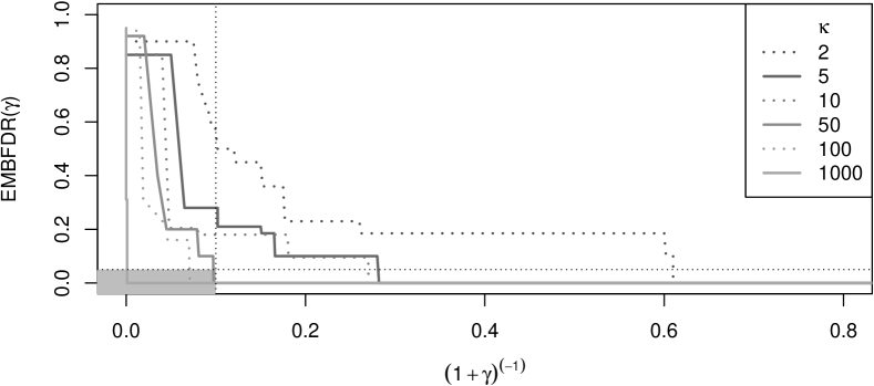
We can now analyze a particular data set using a range of values for $\kappa$ and subsequently make plots of the EMBFDR metric as a function of the threshold ${(1+\gamma)}^{-1}$ or as a function of the proportion of SNPs retained after the EM filter step. Thus, by setting an upper bound for a desired value of the EMBFDR we can investigate these plots and determine an appropriate choice of $\kappa$ and an appropriate range of values of $\gamma$. In Figure 3 we illustrate an application of this criterion. We note that the EMBFDR has broader application to Bayesian variable selection models and can be a useful metric to guide the selection of tuning parameters, in particular the spike-and-slab variance separation parameter $\kappa$.

5.4 Visualizing the relationship between SNPs and genes

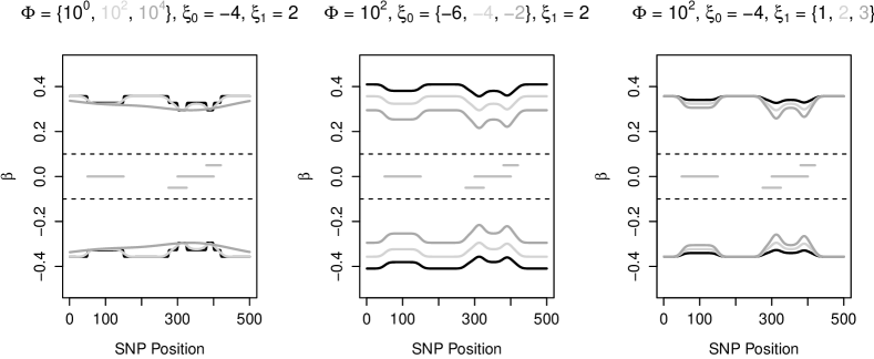
For a given configuration of $\kappa$, $\gamma$, and $\sigma^{2}$, we can plot the bounds $\pm\sigma s_{j}$ on $\beta_{j}$ and inspect the effect of parameters $\phi$, $\xi_{0}$, and $\xi_{1}$. SNPs that are close to relevant genes have thresholds that are relatively lower in magnitude; they need a relatively smaller (in magnitude) coefficient to be selected for the final model. With everything else held fixed, as $\phi\to\infty$ the boost received from the relevant genes will decrease to zero and our model will coincide with a basic version of Bayesian variable selection where $\theta_{j}\stackrel{{\scriptstyle\text{\tiny iid}}}{{\sim}}\text{\sf Bern}({\rm logit}^{-1}(\xi_{0}))$. We demonstrate this visualization on a mock chromosome in Figure 4.

Figure 4: We illustrate the effect of varying $\phi$, $\xi_{0}$ and $\xi_{1}$ on the thresholds on the posterior effect sizes, $\beta_{j}$, in a simple window containing a single gene in isolation, and a group of three overlapping genes. On the left, we vary $\phi$ and control the smoothness of the thresholds. In the middle, we vary $\xi_{0}$ and control the magnitude of the thresholds, or in other words the number of standard deviations ($\sigma$) away from zero at which they are placed. On the right, we vary $\xi_{1}$ and control the sharpness of the difference in the thresholds between differently weighted regions of the window. For this illustration, we set $\sigma^{2}=0.01$, $\kappa=100$, and $\gamma=1$. We mark the distance $\sigma$ away from the origin with black dashed lines.

6 Empirical Studies

We conduct two simulation studies. First, we compare the performance of our method to other well-known methods including single SNP tests, LASSO, fused LASSO, group LASSO, the penalized unified multiple-locus association (PUMA) suite of Hoffman et al. (2013), and the Bayesian sparse linear mixed model (BSLMM) of Zhou et al. (2013). Then we assess the robustness of our method to misspecifications of the range parameter, $\phi$, and gene relevances. We describe each study in detail below, but we first explain how the data is simulated in each scenario.

6.1 Simulation Study Details

To provide a fair comparison across methods and to realistically assess the robustness of our method to misspecifications, we designed our simulation study based on real-life genotypical data and current gene and marker annotations. Specifically, to keep a representative LD structure we sample whole-chromosome individual genotypes by subsampling individual data provided by the 1000 Genomes Project Consortium et al. (2012); gene weights are computed based on gene lengths and positions in the hg19 reference, while marker positions are taken from actual SNP array designs in the WTCCC studies. We consider two studies: a “non-informative” setup where the gene relevances are uniformly set to one and $\phi=10^{8}$, so that marker relevance scores ${\mathbf{w}_{j}(\phi)}^{\top}\mathbf{r}$ are small and close to uniform, and a mild boost effect of $\xi_{1}=1$; and an “informative” study with gene relevances taken as search hit scores from MalaCards (2014) and $\phi=10^{4}$, a frequent value when adopting the procedure in Section 5.1, and a stronger boost effect, $\xi_{1}=5$. These two studies are extreme with respect to marker relevance scores—a function of gene relevances and genomic range—and spatial boost effects and aim at assessing how robust are our model and recommended guidelines. For instance, when fitting all scenarios we take an informative approach by considering the same gene relevances and genomic range from the “informative” scenario, but adopt a conservative approach by setting $\xi_{1}=1$ as in the “non-informative” scenario.

For both studies we simulated two scenarios for the number of markers $p$: the “small” scenario comprised chromosome 19 with $p=4,\!199$ markers, and the “large” scenario containing all $p=28,\!932$ markers in chromosome 2. Chromosomes 19 and 2 are the smallest and largest in terms of number of markers, respectively. We kept the ratio of $p$ to the number of individuals $n$ at $50$, representative of real-life studies, so $n=85$ in the small scenario and $n=580$ in the large scenario. In all simulations we fix the number of causal markers $m=10$ and set the baseline log-odds $\xi_{0}=\lfloor{\rm logit}(m/p)\rfloor$. For each simulation batch, we first sample uniformly at random $n$ individuals from the 1000 Genomes dataset, taking their whole chromosome genotypes according to the small or large scenario, and filter out markers with sampled MAF $<0.05$, deemed as rare variants, or $>0.50$. Next, we sample $m$ causal markers following (3), with marker relevance scores and $\xi_{1}$ taken according to a non-informative or informative scenario. Effect sizes $\beta_{j}$ are then sampled to reflect the challenging nature of GWAS: $\beta_{j}{\,|\,}\theta_{j}\sim\theta_{j}N(0,0.25)+(1-\theta_{j})N(0,0.01)$, that is, small effect sizes for causal markers and relatively large coefficients for noisier non-causal effects. Finally, for each replicate within a batch we sample phenotypes according to (1).

In each simulation scenario and dataset below we fit the model as follows: we adopt informative gene relevances from MalaCards and $\phi=10,\!000$, start with conservative values for the baseline log-odds $\xi_{0}={\rm logit}(100/p)$ and the gene boost effect $\xi_{1}=1$, and run the EM filtering process until either the predictive performance starts degrading or at most $10$ markers remain. We measure predictive performance using a metric similar to posterior predictive loss (PPL; Gelfand and Ghosh, 1998): if, at the $t$-th EM iteration, $\widehat{y}^{(t)}_{i}={\mathbb{E}}[y_{i,\text{rep}}{\,|\,}\widehat{\beta}^{(t)}_{\text{EM}},\mathbf{y}]$ is the $i$-th predicted response, the PPL measure under squared error loss is approximated by

$$\text{PPL}(t)=\sum_{i=1}^{n}{(y_{i}-\widehat{y}_{i})}^{2}+\sum_{i=1}^{n}\text{Var}[y_{i,\mbox{\tiny rep}}{\,|\,}\widehat{\beta}^{(t)}_{EM},\mathbf{y}]=\sum_{i=1}^{n}{(y_{i}-\widehat{y}_{i})}^{2}+\widehat{y}_{i}(1-\widehat{y}_{i}).$$

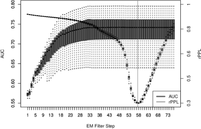
The right panel in Figure 5 shows an example of how the relative PPL (rPPL) typically varies as the EM filter advances. We define the rPPL at the $t$-th EM iteration as the ratio between PPL$(t)$ and the PPL of the null model, that is, the model with only the intercept and no marker genotypes as predictors. At the end of the filtering stage we run the Gibbs sampler with $\xi_{0}={\rm logit}(m/\widetilde{p})$, where $\widetilde{p}$ is the number of markers retained at the end of the EM filter. Parameter $\kappa$ is actually elicited at each EM filtering iteration using EMBFDR.

6.2 Comparison Simulation Study

In this study, we generated 10 batches of simulated data, each containing 5 replicates, for a total of 50 simulated data sets for each cross configuration of small and large scenarios by non-informative and informative studies. After simulating the data, we fit our model and compared its performance in terms of area under the receiver operating characteristic (ROC) curve (AUC) to the usual single SNP tests, LASSO, fused LASSO, group LASSO, PUMA, and BSLMM methods. We used the penalized package in R to fit the LASSO and fused LASSO models; we used ten-fold cross-validation to determine the optimal values for the penalty terms. Similarly, we used the gglasso package in R to fit the group LASSO model where we defined the groups such that any two adjacent SNPs belonged to the same group if they were within $10,\!000$ base pairs of each other; we used ten-fold cross validation to determine the optimal value for the penalty term. Finally, we used the authors’ respective software packages to fit the PUMA and BSLMM models.

To calculate the AUC for any one of these methods, we took a final ranking of SNPs based on an appropriate criterion (see more about this below), determined the points on the ROC curve using our knowledge of the true positives and the false positives from the simulated data, and then calculated the area under this curve. For our model, we used either the ranking (in descending order) of $\mathbb{E}[\theta_{j}{\,|\,}\widehat{\beta}_{\text{EM}},\widehat{\sigma}^{2}_{\text{EM}},y]$ for a particular EM filtering step or $\widehat{\mathbb{P}}(\theta_{j}=1{\,|\,}y)$ using the samples obtained by the Gibbs sampler; for the single SNP tests we used the ranking (in ascending order) of the p-values for each marker’s test; for LASSO, fused LASSO and group LASSO we used the ranking (in descending order) of the magnitude of the effect sizes of the SNPs in the final model; for the other penalized regression models given by the PUMA program, we used the provided software to compute p-values for each SNP’s significance in the final model and used the ranking (in ascending order) of these p-values; for BSLMM we used the ranking (in descending order) of the final estimated posterior probabilities of inclusion for each SNP in the final model.

The left panel in Figure 5 shows examples of ROC curves from a random simulation replicate. Since the interest in GWA studies is focused on low false positive rates, we also evaluate the performance of the methods with respect to relative AUC (rAUC) at some false positive rate $f$, defined simply as the normalized AUC up to FPR $f$, that is, rAUC$(f)$ = AUC$(f)/f$. According to this criterion, the solid ROC curve in Figure 5 has a clearer advantage over the dashed curve at a 10% FPR. The right panel illustrates how the AUC changes with rPPL and as the EM filtering iterations increase.

Figure 5: Left: examples of ROC curves for our method (solid line for EM results, crosses for Gibbs sampling results) and single SNP tests (dashed line); vertical gray line marks a false positive rate of 10%. Right: relation between AUC and relative PPL (rPPL) as the EM filter progresses, boxplots over replicates within a simulation batch; in this case the EM filter would stop at iteration 58, right before rPPL starts increasing.

We summarize the results in Figure 6. With respect to AUC (top four panels), our methods perform better on average than the other methods in the informative scenario, but only comparably in the non-informative scenario. Note that all models have a modest performance due to the challenging nature of the simulation (but our model has improved performance under less stringent scenarios; see LABEL:suppA for more details). Most of the gain in our methods comes at the beginning of the ROC curves, i.e. at low false positive rates, as exemplified in Figure 5. This becomes more evident if we compare relative AUC in the bottom four panels. We note that the gains are present even in the “null” models with $\xi_{1}=0$, so they stem from the joint modeling of markers. Additional gains in rAUC are more apparent in the informative scenario (bottom row).

Figure 6: Results from the comparison simulation study. Top four panels show AUC, while bottom four panels show relative AUC. Within each block of four panels: left panels show results under non-informative scenario (top) and informative scenario (bottom) for small study, while right panels show respective AUC or rAUC results for the large study. The boxplots in each panel are, left to right: single SNP (SS) tests; spatial boost “null” (no boost) model at the first (EM₀) and last (EM_∞) iteration of the EM filter and after Gibbs sampling phase; spatial boost “informative” model at first and last EM filtering iterations and after Gibbs sampling phase; LASSO (L); fused LASSO (L_f); grouped LASSO (L_g); PUMA with penalties NEG, LOG, MCP, and adaptive LASSO (L_a); and BSLMM (B).

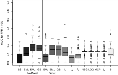
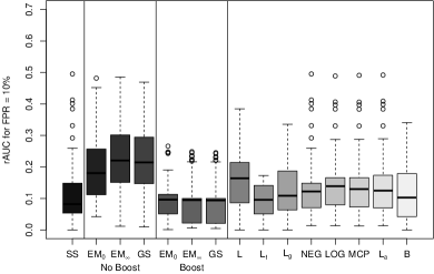
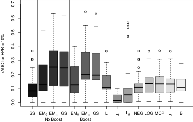
The seemingly bad performance of our model in the non-informative scenario indicates that the model can be sensitive to poor marker relevance scores, arising either from meaningless gene relevances or a non-representative genomic range $\phi$. This is not surprising given that the inference relies on good prior information in the large-$p$-small-$n$ regimen; however, as the informative scenario suggests, the model is more robust to misspecification of $\xi_{1}$, which can be seen as the overall prior strength of relevance scores. The null model, for instance, often offers the best performances in both AUC and relative AUC, which recommends conservative, low values for $\xi_{1}$ in initial analyses. Moreover, the EM filtering procedure contributes to further gains in performance even in non-informative scenarios, that is, with misspecified relevance scores. These gains are even more pronounced with larger causal effect sizes relative to non-causal effects, as we show in LABEL:suppA; that is, we observe that the EM filter becomes more robust to these misspecifications, especially on large scenarios and under low false positive rates, as shown here.

6.3 Relevance Robustness Simulation Study

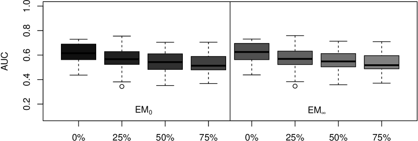
To investigate how robust our model is to misspecifications of gene relevances and genomic range, we focus on their joint effect in defining marker relevance scores and again consider the small (chromosome 19) and large (chromosome 2) scenarios under the informative study, where the gene relevances are more varied. We randomly select one batch from the comparison study to be the reference in each scenario, with its replicates serving as ground truth. We then vary three sampling percentages $\pi\in\{25\%,50\%,75\%\}$, and, for each $\pi$, we randomly select $\lfloor\pi p\rfloor$ markers uniformly from each reference replicate and sample their relevance scores from the empirical distribution of relevance scores in each scenario. This simulation is replicated 50 times.

Hyper-prior parameters $\xi_{0}$, $\xi_{1}$, and $\kappa$ were elicited as in Section 6.1. For each simulated replication we then fit our model and assess performance using the AUC, as in the previous study. Figure 7 illustrates the distribution of relevance scores for the markers in chromosomes 19 and 2 and how the performance of the model varies at each sample percentage. The AUC at initial EM iterations degrades with higher percentages for both scenarios, as expected; however, small scenario replicates continue to show a similar pattern at their last EM iterations, as opposed to large scenario replicates that show better and stable results across all percentages. We attribute this discrepancy in robustness to the distribution of relevance scores. As the left panel in Figure 7 shows, the large scenario has a bimodal distribution and low mean score and so a few markers are relevant; in contrast, the small scenario score distribution has more spread and higher mean and so many markers can be relevant and influence negatively the fit by calling more false positives. We thus recommend to analyze the resulting distribution of marker relevance scores when eliciting gene relevances and $\phi$.

Figure 7: Results from the simulation study to assess robustness to marker relevance scores. Left panel shows the distribution of marker relevance score from small and large scenarios, chromosomes 19 and 2, respectively. Right panels show AUC results for first (EM₀) and last (EM_∞) filtering iterations across simulation percentages for small (top) and large (bottom) scenarios. Null percentages correspond to reference replicates.

7 Case Study

Using data provided by the WTCCC, we analyzed the entire genome (342,502 SNPs total) from a case group of 1,999 individuals with rheumatoid arthritis (RA) and a control group of 1,504 individuals from the 1958 National Blood Bank dataset. For now we addressed the issues of LD, rare variants, and population stratification by analyzing only the SNPs in Hardy-Weinberg Equilibrium (Wigginton et al., 2005) with minor allele frequency greater than 5%. There are 15 SNPs that achieve genome-wide significance when using a Bonferroni multiple testing procedure on the results from a single SNP analysis. Table 1 in LABEL:suppA provides a summary of these results for comparison to those obtained when using the spatial boost model.

When fitting the spatial boost model, we broke each chromosome into blocks and selected an optimal value of $\phi$ for each block using our proposed method metric, $|\rho_{i,j}|(\phi)$. We used the EMBFDR to select a choice for $\kappa$ from the set $\{10^{2},10^{3},10^{4},10^{5},10^{6}\}$ at each step of our model fitting pipeline so that the BFDR was no greater than 0.05 while retaining no larger than 5% of the total number of SNPs. With a generous minimum standard deviation $s=1$ we have that trivially $\xi_{0}<0$ from (13), but we set $\xi_{0}=-8$ to encode a prior belief that around 100 markers would be associated to the trait on average a priori. The bound on $\xi_{1}$ is then $\xi_{1}\leq 8$, but we consider log odds-ratio boost effects of $\xi_{1}\in\{1,4,8\}$. A value of $\xi_{1}=1$ is more representative of low power GWA studies; however, the larger boost effects offer more weight to our prior information. For comparison, we also fit a model without any gene boost by setting $\xi_{1}=0$ (the “null” model), and also fit two models for each possible value of $\xi_{1}$ trying both a non-informative gene relevance vector and a vector based on text-mining scores obtained from MalaCards (2014).

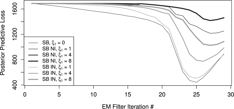
To accelerate the EM algorithm, we rank-truncate $X$ using $l=3,\!259$ singular vectors; the mean squared error between $X$ and this approximation is less than 1%. We apply the EM filtering 29 times and use PPL to decide when to start the Gibbs sampler. As Figure 8 shows, in all of our fitted models, the PPL decreases slowly and uniformly for the first twenty or so iterations, and then suddenly decreases more sharply for the next five iterations until it reaches a minimum and then begins increasing uniformly until the final iteration, similarly to the behavior depicted in Figure 5. For comparison to the 15 SNPs that achieve genome-wide significance in the single marker tests, Tables 2-15 in LABEL:suppA list, for each spatial boost model, the top 15 SNPs at the optimal EM filtering step, i.e. the step with the smallest PPL, and the top 15 SNPs based on the posterior samples from our Gibbs sampler when using only the corresponding set of retained markers.

Figure 8: Although we run the EM filter until the number of retained markers $<$ 100 (iteration #29), the PPL metric often tells us to keep between 200 to 250 markers (iterations #25–26).

We observe the most overlap with the results of the single SNP tests in our null model where $\xi_{1}=0$ and in our models that use informative priors based on relevance scores from MalaCards. Although there is concordance between these models in terms of the top 15 SNPs, it is noteworthy that we select only a fraction of these markers after running either the EM algorithm or the Gibbs sampler. Based on the results from our simulation study where we observe superior performances for the spatial boost model at low false positive rates, we believe that an advantage of our method is this ability to highlight a smaller set of candidate markers for future investigation.

Indeed, after running our complete analysis, we observe that the usual threshold of $0.5$ on $\widehat{\mathbb{P}}(\theta_{j}=1|y)$ would result in only the null spatial boost model ($\xi_{1}=0$), the low gene boost non-informative model ($\xi_{1}=1$), and the informative models selecting SNPs for inclusion in their respective final models. The SNPs that occur the most frequently in these final models are the first four top hits from the single SNP tests: rs4718582, rs10262109, rs6679677, and rs664893. The SNP with the highest minor allele frequency in this set is rs6679677; this marker has appeared in several top rankings in the GWAS literature (e.g. (Burton et al., 2007)) and is in high LD with another SNP in gene PTPN22 which has been linked to RA (Michou et al., 2007).

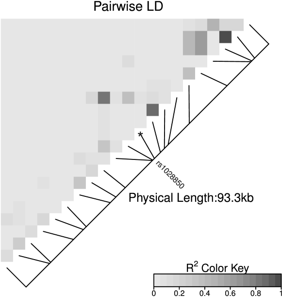
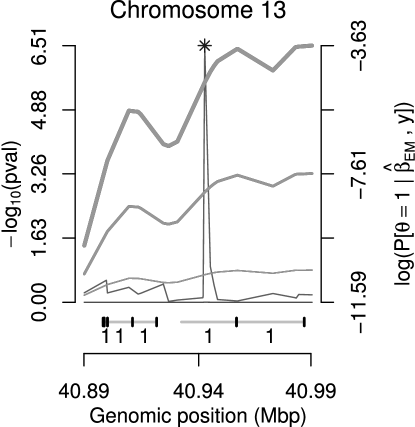
If we consider only the final models obtained after running the EM filter, we see another interesting SNP picked up across the null and informative models: rs1028850. In Figure 9, we show a closer look at the region around this marker and compare the trace of the Manhattan plot with the traces of each spatial boost model’s $\mathbb{E}[\theta_{j}|\widehat{\beta}_{EM},\widehat{\sigma}^{2}_{\text{EM}},y]$ values at the first iteration of the EM filter. To the best of our knowledge this marker has not yet been identified as being associated to RA; moreover, it is located inside a non-protein coding RNA gene, LINC00598, and is close to another gene that has been linked to RA, FOXO1 (Grabiec et al., 2014).

As we increase the strength of the gene boost term with a non-informative relevance vector, the relatively strong prior likely leads to a mis-prioritization of all SNPs that happen to be located in regions rich in genes. In the supplementary tables (2-15) of LABEL:suppA we list the lengths of the genes that contain each SNP and we see that indeed the non-informative gene boost models tend to retain SNPs that are near large genes that can offer a generous boost. Perhaps due to prioritizing the SNPs incorrectly in these models, we do not actually select any markers at either the optimal EM filtering step or after running the Gibbs sampler. However, some of the highest ranking SNPs for these models, rs1982126 and rs6969220, are located in gene PTPRN2 which is interestingly a paralog of PTPN22.

Figure 9: Although rs1028850 has a relative peak in the Manhattan plot (SS), it does not achieve genome-wide significance. The spatial boost (SB) model initially prioritizes markers that are closer to the center of regions rich in genes, but selects rs1028850 for inclusion in the final model by the end of the EM filter (not shown) under several configurations.

8 Conclusions

We have presented a novel hierarchical Bayesian model for GWAS that exploits the structure of the genome to define SNP-specific prior distributions for the model parameters based on proximities to relevant genes. While it is possible that other “functional” regions are also very relevant—e.g. regulatory and highly conserved regions—and that mutations in SNPs influence regions of the genome much farther away—either upstream, downstream, or, through a complex interaction of molecular pathways, even on different chromosomes entirely—we believe that incorporating information about the genes in the immediate surroundings of a SNP is a reasonable place to start.

By incorporating prior information on relevant genomic regions, we focus on well annotated parts of the genome and were able to identify, in real data, markers that were previously identified in large studies and highlight at least one novel SNP that has not been found by other models. Clearly, validation via other studies of the importance of this marker for RA should be investigated. In addition, as shown in a simulation study, while logistic regression under large-$p$-small-$n$ regimen is challenging, the spatial boost model often outperforms simpler models that either analyze SNPs independently or employ a uniform penalty term on the $L_{1}$ norm of their coefficients.

Our main point is that we regard a fully joint analysis of all markers as essential to overcome genotype correlations and rare variants. This approach, however, entails many difficulties. From a statistical point of view, the problem is severely ill-posed so we rely on informative, meaningful priors to guide the inference. From a computational perspective, we also have the daunting task of fitting a large scale logistic regression, but we make it feasible by reducing the dimension of both data—intrinsically through rank truncation—and parameters—through EM filtering. Moreover, from a practical point of view, we provide guidelines for selecting hyper-priors, reducing dimensionality, and implement the proposed approach using parallelized routines.

From the simulation studies in Section 6 we can further draw two conclusions. First, as reported by other methods such as PUMA, filtering is important; our EM filtering procedure seems to focus on effectively selecting true positives at low false positive rates. This feature of our method is encouraging, since practitioners are often interested in achieving higher sensitivity by focusing on lower false positive rates. Second, because we depend on good informative priors to guide the selection of associated markers, we rely on a judicious choice of hyper-prior parameters, in particular of the range parameter $\phi$ and how it boosts markers within neighboring genes that are deemed relevant. It is also important to elicit gene relevances from well curated databases, e.g. MalaCards, and to calibrate prior strength according to how significant these scores are.

We have shown that our model performs better than most variable selection methods, but that it can suffer in case of severe model misspecification. As a way to flag misspecification we suggest to check monotonicity in a measure of model fit such as PPL as we filter markers using EM. In addition, refining the EM filtering by using a lower threshold ($<.25$) at each iteration can help increase performance, especially at lower false positive rates.

When applying the spatial boost model to a real data set, we were able to confidently isolate at least one marker that has previously been linked to the trait as well as find another novel interesting marker that may be related to the trait. This shows that although we can better explore associations jointly while accounting for gene effects, the spatial boost model still might lack power to detect associations between diseases and SNPs due to the high correlation induced by linkage disequilibrium. In the future we plan to increase the power even further by extending the model to include a data pre-processing step that attempts to formally correct for the collinearity between SNPs.

References

- 1000 Genomes Project Consortium et al. (2012) 1000 Genomes Project Consortium et al. (2012). An integrated map of genetic variation from 1,092 human genomes. Nature 491(7422), 56–65.
- Al-Mubaid and Singh (2010) Al-Mubaid, H. and R. K. Singh (2010). A text-mining technique for extracting gene-disease associations from the biomedical literature. International journal of bioinformatics research and applications 6(3), 270–286.
- Balding (2006) Balding, D. J. (2006). A tutorial on statistical methods for population association studies. Nature Reviews Genetics 7(10), 781–791.
- Bansal et al. (2010) Bansal, V., O. Libiger, A. Torkamani, and N. J. Schork (2010). Statistical analysis strategies for association studies involving rare variants. Nature Reviews Genetics 11(11), 773–785.
- Barbieri and Berger (2004) Barbieri, M. and J. Berger (2004). Optimal predictive model selection. The Annals of Statistics 32(3), 870–897.
- Berger (1985) Berger, J. (1985). Statistical decision theory and Bayesian analysis. Springer.
- Burton et al. (2007) Burton, P. R., D. G. Clayton, L. R. Cardon, N. Craddock, P. Deloukas, A. Duncanson, D. P. Kwiatkowski, M. I. McCarthy, W. H. Ouwehand, N. J. Samani, et al. (2007). Genome-wide association study of 14,000 cases of seven common diseases and 3,000 shared controls. Nature 447(7145), 661–678.
- Carvalho and Lawrence (2008) Carvalho, L. and C. Lawrence (2008). Centroid estimation in discrete high-dimensional spaces with applications in biology. Proceedings of the National Academy of Sciences 105(9), 3209–3214.
- Cowles and Carlin (1996) Cowles, M. K. and B. P. Carlin (1996). Markov chain monte carlo convergence diagnostics: a comparative review. Journal of the American Statistical Association 91(434), 883–904.
- Dempster et al. (1977) Dempster, A. P., N. M. Laird, and D. B. Rubin (1977). Maximum likelihood from incomplete data via the EM algorithm. Journal of the Royal Statistical Society. Series B (Methodological) 39(1), 1–38.
- Evangelou and Ioannidis (2013) Evangelou, E. and J. P. Ioannidis (2013). Meta-analysis methods for genome-wide association studies and beyond. Nature Reviews Genetics 14(6), 379–389.
- Friedman et al. (2010) Friedman, J., T. Hastie, and R. Tibshirani (2010, Jan). A note on the group lasso and a sparse group lasso. Technical Report arXiv:1001.0736, Stanford University.
- Gelfand and Ghosh (1998) Gelfand, A. E. and S. K. Ghosh (1998). Model choice: A minimum posterior predictive loss approach. Biometrika 85(1), 1–11.
- George and McCulloch (1993) George, E. I. and R. E. McCulloch (1993). Variable selection via gibbs sampling. Journal of the American Statistical Association 88(423), 881–889.
- Grabiec et al. (2014) Grabiec, A. M., C. Angiolilli, L. M. Hartkamp, L. G. van Baarsen, P. P. Tak, and K. A. Reedquist (2014). JNK-dependent downregulation of FoxO1 is required to promote the survival of fibroblast-like synoviocytes in rheumatoid arthritis. Annals of the Rheumatic Diseases 74(9), annrheumdis–2013.
- Guan and Stephens (2011) Guan, Y. and M. Stephens (2011). Bayesian variable selection regression for genome-wide association studies and other large-scale problems. The Annals of Applied Statistics 5(3), 1780–1815.
- Habier et al. (2011) Habier, D., R. Fernando, K. Kizilkaya, and D. Garric (2011). Extension of the Bayesian alphabet for genomic selection. BMC bioinformatics 12, 186.
- Hamada and Asai (2012) Hamada, M. and K. Asai (2012). A classification of bioinformatics algorithms from the viewpoint of maximizing expected accuracy (MEA). Journal of Computational Biology 19(5), 532–549.
- Haupt et al. (2011) Haupt, J., R. M. Castro, and R. Nowak (2011). Distilled sensing: Adaptive sampling for sparse detection and estimation. Information Theory, IEEE Transactions on 57(9), 6222–6235.
- Heard et al. (2010) Heard, E., S. Tishkoff, J. A. Todd, M. Vidal, G. P. Wagner, J. Wang, D. Weigel, and R. Young (2010). Ten years of genetics and genomics: what have we achieved and where are we heading? Nature Reviews Genetics 11(10), 723–733.
- Hoerl and Kennard (1970) Hoerl, A. and R. Kennard (1970). Ridge regression - applications to nonorthogonal problems. Technometrics 12, 69–82.
- Hoffman et al. (2013) Hoffman, G. E., B. A. Logsdon, and J. G. Mezey (2013). Puma: a unified framework for penalized multiple regression analysis of gwas data. PLoS computational biology 9(6), e1003101.
- Ioannidis et al. (2009) Ioannidis, J. P., G. Thomas, and M. J. Daly (2009). Validating, augmenting and refining genome-wide association signals. Nature Reviews Genetics 10(5), 318–329.
- Ishwaran and Rao (2005) Ishwaran, H. and J. S. Rao (2005). Spike and slab variable selection: Frequentist and Bayesian strategies. Annals of Statistics 33(2), 730–773.
- Jorgenson and Witte (2006) Jorgenson, E. and J. S. Witte (2006). A gene-centric approach to genome-wide association studies. Nature Reviews Genetics 7(11), 885–891.
- Kooperberg et al. (2010) Kooperberg, C., M. LeBlanc, and V. Obenchain (2010). Risk prediction using genome-wide association studies. Genetic epidemiology 34(7), 643–652.
- MacCullagh and Nelder (1989) MacCullagh, P. and J. A. Nelder (1989). Generalized linear models, Volume 37. CRC press.
- MalaCards (2014) MalaCards (2014). Genes related to rheumatoid arthritis. http://www.malacards.org/card/rheumatoid_arthritis. [Online, accessed 2014-10-01].
- McCullagh and Nelder (1989) McCullagh, P. and J. A. Nelder (1989). Generalized Linear Models. London England Chapman and Hall 1983.
- Meng and Rubin (1993) Meng, X.-L. and D. B. Rubin (1993). Maximum likelihood estimation via the ECM algorithm: A general framework. Biometrika 80(2), 267–278.
- Michou et al. (2007) Michou, L., S. Lasbleiz, A.-C. Rat, P. Migliorini, A. Balsa, R. Westhovens, P. Barrera, H. Alves, C. Pierlot, E. Glikmans, et al. (2007). Linkage proof for ptpn22, a rheumatoid arthritis susceptibility gene and a human autoimmunity gene. Proceedings of the National Academy of Sciences 104(5), 1649–1654.
- Mitchell and Beauchamp (1988) Mitchell, T. J. and J. J. Beauchamp (1988). Bayesian variable selection in linear regression. Journal of the American Statistical Association 83(404), 1023–1032.
- Peng et al. (2013) Peng, B., D. Zhu, B. P. Ander, X. Zhang, F. Xue, F. R. Sharp, and X. Yang (2013). An integrative framework for bayesian variable selection with informative priors for identifying genes and pathways. PloS one 8(7), e67672.
- Petersen and Pedersen (2008) Petersen, K. B. and M. S. Pedersen (2008). The matrix cookbook.
- Polson et al. (2013) Polson, N., J. Scott, and J. Windle (2013). Bayesian inference for logistic models using Pólya-Gamma latent variables. Journal of the American Statistical Association 108(504), 1339–1349.
- Pritchard and Przeworski (2001) Pritchard, J. and M. Przeworski (2001). Linkage disequilibrium in humans: Models and data. American Journal of Human Genetics 69, 1–14.
- Stephens and Balding (2009) Stephens, M. and D. J. Balding (2009). Bayesian statistical methods for genetic association studies. Nature Reviews Genetics 10(10), 681–690.
- Technology Department Carnegie Library of Pittsburgh (2002) Technology Department Carnegie Library of Pittsburgh (2002). The Handy Science Answer Book. Visible Ink Press.
- Tibshirani (1996) Tibshirani, R. (1996). Regression shrinkage and selection via the lasso. Journal of the Royal Statistical Society 58, 267–288.
- Tibshirani and Saunders (2005) Tibshirani, R. and M. Saunders (2005). Sparsity and smoothness via the fused lasso. Journal of the Royal Statistical Society 67, 91–108.
- Wang et al. (2005) Wang, W. Y., B. J. Barratt, D. G. Clayton, and J. A. Todd (2005). Genome-wide association studies: theoretical and practical concerns. Nature Reviews Genetics 6(2), 109–118.
- West (2003) West, M. (2003). Bayesian factor regression models in the “large p, small n” paradigm. Bayesian Statistics 7(2003), 723–732.
- Whittemore (2007) Whittemore, A. S. (2007). A bayesian false discovery rate for multiple testing. Journal of Applied Statistics 34(1), 1–9.
- Wigginton et al. (2005) Wigginton, J. E., D. J. Cutler, and G. R. Abecasis (2005). A note on exact tests of hardy-weinberg equilibrium. The American Journal of Human Genetics 76(5), 887–893.
- Wu et al. (2010) Wu, M. C., P. Kraft, M. P. Epstein, D. M. Taylor, S. J. Chanock, D. J. Hunter, and X. Lin (2010). Powerful snp-set analysis for case-control genome-wide association studies. The American Journal of Human Genetics 86(6), 929–942.
- Wu et al. (2011) Wu, M. C., S. Lee, T. Cai, Y. Li, M. Boehnke, and X. Lin (2011). Rare-variant association testing for sequencing data with the sequence kernel association test. The American Journal of Human Genetics 89(1), 82–93.
- Zhou et al. (2013) Zhou, X., P. Carbonetto, and M. Stephens (2013). Polygenic modeling with bayesian sparse linear mixed models. PLoS genetics 9(2), e1003264.
- Zou and Hastie (2005) Zou, H. and T. Hastie (2005). Regularization and variable selection via the elastic net. Journal of the Royal Statistical Society 67, 301–320.