Structured functional regression models
for high-dimensional spatial spectroscopy data

Abstract

Modeling and analysis of spectroscopy data is an active area of research with applications to chemistry and biology. This paper focuses on analyzing Raman spectra obtained from a bone fracture healing experiment, although the functional regression model for predicting a scalar response from high-dimensional tensors can be applied to any spectroscopy data. The regression model is built on a sparse functional representation of the spectra, and accommodates multiple spatial dimensions. We apply our models to the task of predicting bone-mineral-density (BMD), an important indicator of fracture healing, from Raman spectra, in both the in vivo and ex vivo settings of the bone fracture healing experiment. To illustrate the general applicability of the method, we also use it to predict lipoprotein concentrations from spectra obtained by nuclear magnetic resonance (NMR) spectroscopy.

1 Introduction

Spectroscopy is a type of chemical analysis that infers the composition of a specimen by using information revealed when it interacts with radiated energy. Spectroscopic imaging extends the utility of traditional spectroscopy by using spectra obtained for multiple spatial locations within a specimen to map the spatial distributions of its chemical constituents. Since some forms of spectroscopy can be carried out non-invasively and without exposing research subjects to hazards such as ionizing radiation or chemical tracers, potential uses of spectroscopy in medical imaging and diagnostic testing are being actively explored.

Raman spectroscopy is a type of spectroscopy that is based on inelastic light scattering [5]. Like other more familiar forms of spectroscopy such as infrared (IR) and nuclear magnetic resonance (NMR/SMR) spectroscopy, Raman spectroscopy produces a spectrum that expresses the intensity of Raman scattering at each wavelength. This spectrum encodes the chemical structure of the specimen. Raman spectroscopy uses laser light as an energy source and is relatively inexpensive compared to MR spectroscopy. However, the signal strength for Raman spectroscopy is low, and for human or animal subjects images can only be acquired at the depth to which the laser light can penetrate the body. Raman imaging can be used to image through thin layers of skin and connective tissue. For example, Raman maps of bone composition in the human wrist area, or in limbs of small animals, can be obtained non-invasively using transcutaneous Raman imaging [9].

Both Raman and MR spectra exhibit a linearity property that allows the chemical composition of a complex mixture of pure components to be resolved. The measured spectrum of a sample composed of multiple chemical constituents is approximately equal to the weighted pointwise sum of the pure component spectra, weighted by the abundance of each component within the specimen. An extensive literature in statistics and chemometrics [3, 18, 8, 12, 17] has focused on techniques for resolving the pure component spectra, and for quantifying the abundance of each constituent within a specimen. Much of this work focuses on analyzing collections of individual spectra, rather than on spatial maps.

Many promising applications of spectroscopy involve assesment of biological specimens for diagnostic purposes. Raman maps of bone composition obtained at the wrist may provide a useful imaging biomarker for early detection of bone diseases such as osteoarthritis, or to non-invasively monitor bone healing following a fracture [14, 9]. In another context, NMR spectroscopy has been used to quantify the lipoprotein fractions in plasma samples [4]. These can both be viewed as prediction problems, in which the information to be used for prediction is either a single spectrum or a collection of spectra. This prediction problem can be approached by applying regression techniques to relate the clinical outcomes to the raw spectra, using a training set of labeled data. Alternatively, a more mechanistic approach can be used in which chemical signatures known to be related to the variable of interest, such as mineral components in the spectrum of a healing fracture, are used to predict the outcome. This approach is often guided by external information in the form of libraries of pure bone and tissue spectra, obtained ex vivo from similar specimens. For recent advances in this line of work, we refer to [7].

The motivation for the models to be discussed in this paper is a more challenging task of estimating bone composition from Raman data collected around a larger body part, e.g., around the leg of a rat. The difficulty in this case is that the non-negligible amount of tissue surrounding the bone contributes components to the spectrum. Due to this mixing of signals from bone and tissue, and the weakness of the Raman signal, it is not yet known whether bone composition can be accurately predicted from such in vivo Raman readings, and we are not aware of existing successful attempts to predict an objective measure of bone composition solely from in vivo Raman data.

In this study, we focus on predicting bone-mineral-density (BMD) obtained by micro-CT scans as a “gold standard” for bone composition and fracture healing (see more on the study set-up in Section 2. The BMD is an important predictor of fracture healing, and micro-CT scans are a very accurage way to estimate the BMD, but they are expensive and involve higher doses of radiation.

We propose a regularized regression approach for using spectroscopic images for prediction. Framing the analysis in a predictive context, rather than as separate feature extraction and modeling stages, leads to the discovery of image features that are specifically targetted to the predictive task. However this leads to a very high dimensional regression (e.g. the Raman imaging study discussed below has $544\times 10\times 5$ features and 37 independent samples), so some form of regularization is essential. We propose the use of several regularizers that respect both the functional forms of individual spectra, and the way in which the multiple observed spectra for each subject are related.

The paper is organized as follows. In Section 2, we outline the setup for a fracture healing experiment, in which spatial in vivo Raman data were obtained from a collection of rats, with the aim of predicting progression of healing. Since our models are mainly motivated by the data from this experiment, we will discuss the setup and the nature of the data in some detail. However, the models are general and can be applied in other spectroscopy settings. As a further example, we also consider the ex vivo Raman microscopy data from the same fracture healing experiment. The ex vivo data have higher signal-to-noise than the in vivo data and are expected to provide much more accurate estimates of the BMD, however, they lack the rich spatial structure of the in vivo data, and also of course obtaining ex vivo data requires sacrificing the animals and is of no use as a diagnostic tool. Another type of spectroscopy where our models can be beneficial is NMR, and we briefly demonstrate their application to a NMR experiment.

Section 3 is devoted to the discussion of our models. We first propose, in Section 3.1, a representation of the data which takes into account its functional nature. The representation, based on a functional version of the Lasso [15], simultaneously achieves denoising and compression. Our main regression model, discussed in Section 3.2, builds on the functional representation and takes into account the tensor aspect of the data. In Section 4, we report some empirical results regarding application of the models to the three datasets described in Section 2. The paper concludes, in Section 5 with a discussion of present shortcomings and possible extensions of this work.

2 Experimental data

2.1 In vivo Raman data

The models in this paper are primarily motivated by the Raman data from a bone fracture healing experiment. The study was conducted on $30$ rats. Each rat underwent a surgical procedure to induce a small defect in one of its tibias, removing a thin slice of bone and fixing the bone to a metal plate so that it can heal back. The rats were then monitored for an eight-week period, at two-week intervals, starting from week 2. Six rats were sampled at all the four time points, while the rest were only sampled at a single time point (either at week 2, 4, 6 or 8) and then sacrificed to collect ex vivo Raman and micro-CT data. We have discarded week 2 data, due to equipment calibration issues that were resolved later. In total, $n=37$ usable rat-week samples are available for the analysis.

In order to collect the Raman spectra, a ring-shaped apparatus was devised, a schematic of which is illustrated in Figure 1. The ring has $d=10$ holes around its circumference, such that either an illumination or a detection fiber can be inserted into each hole. The illumination (source) fiber emits laser light, and the detection fibers capture the resulting scattered light. At any given time, only one illumination fiber is used, and the remaining holes contain detection fibers.

Figure 1: A schematic of the ring-shaped apparatus used for obtaining the in vivo Raman data from across the leg of a rat.

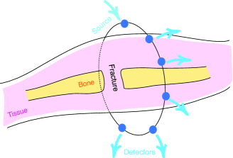
To obtain each Raman measurement, the ring is placed around the leg of the rat, aligned with the defect, the source is placed in some position, the scattered light is collected, and the process is repeated by moving the source to a different position. In total, the source assumes $p=5$ positions around the periphery of the ring.

The spectra produced at each of the detector positions are waveforms expressing the intensity of incident scattered light for wavenumbers approximately in the range from $954\text{\,}\mathrm{c}\mathrm{m}^{-1}$ to $1800\text{\,}\mathrm{c}\mathrm{m}^{-1}$. We have truncated the upper end of the spectrum around $1700\text{\,}\mathrm{c}\mathrm{m}^{-1}$ point, since there is thought to be little relevant information beyond that point. The total number of wavenumbers, after truncation, is $N=544$.

Figure 2: Ring view of in vivo Raman tensor for each of the $p=5$ source positions. Each cylinder represents all the spectra collected for a particular source. The dimension that goes into the page represents the wavenumber. The dots around the ring correspond (roughly) to detector positions (one of which is also a source position in each case.)

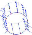
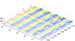
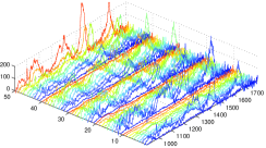
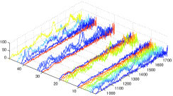
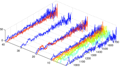
To summarize, the data for each rat obtained on a single measurement occasion can be viewed as a $544\times 10\times 5$ array, with the first dimension corresponding to wavenumbers, the second to the receiver position, and the third to the source position. Figure 2 visualizes these data by placing each detector waveform at the corresponding position around the ring. Note that as the source rotates, the location of the highest amplitude detector rotates too. In general, the closer the detector is to the source, the larger is the amplitude of its waveform. Figure 3 is another visualization of a single measurement, where the source and detector dimensions are stacked to obtain a $544\times 50$ matrix. The four different plots in Figure 3 show the same measurement at different scales. In each plot, the spectra whose amplitude exceeds the scale are omitted from the plot.

Figure 3 clearly shows the need for normalization. Different source-detector combinations produce spectra of highly different amplitudes, which cannot be explained by the relative source/detector positions. Also, though not visible in the figure, there is variability betweeen different measurement times. That is, on different occasions, the same source-detector combination might exhibit different gains (leading to a different overall amplitude each time). It is clear that one needs some form of normalization to combine spectra of such variable scale. Normalization is addressed in our model by assigning a coefficient to each source and each detector, so that a proper normalization is learned from the data. We also employ some simple a priori normalization before applying the model as a form of pre-processing. At the experimental level, normalization can be addressed by embedding some form of reference in the sample, to be used later for calibration. This is often done by using, for example, a polymer fiber which produces a strong Raman signal for the polymer itself. The drawback is some interference with Raman signal of interest from bone and tissue, and this method was not used in our study.

Another issue seen especially in Figure 3 is the presence of some weak waveforms (cf. the bottom right plot) that do not exhibit the overall pattern of a Raman spectrum. These might be due to the detector being out of position (not properly touching the tissue) or the source-detector positions being far apart, leading to a low signal-to-noise ratio. It is desirable to have an automatic procedure for discarding these noise spectra. Our model addresses this issue, to some extent, by picking the relevant source-detector combinations. This is another consequence of assigning a coefficient to each source and detector, and estimating them based on the data. A third issue illustrated by Figure 3, is the noisy nature of Raman data, which is especially evident at lower scales, suggesting that some form of denoising might be helpful. This will be automatically handled by our functional representation, to be discussed in Section 3.1

Our main goal for the Raman data from this experiment is to test its ability to predict well-established biomarkers of fracture healing which can be obtained by the more costly micro-CT approach. The mirco-CT data is obtained ex vivo, and it can produce measures such as bone mineral content (BMC), bone mineral density (BMD), tissue mineral content (TMC), and tissue mineral density (TMD). Although the micro-CT data can produce a high-resolution spatial map of these quantities inside the specimen, we only had access to an average value for each rat within the region of interest. The different markers are highly correlated and we have elected to consider only the BMD sequence. Thus, our response is a sequence of $n=37$ scalar BMD measurements. In Section 3.2, we will discuss our regression model relating the Raman tensor to the BMD response.

Figure 3: Flattened view of the in vivo Raman tensor. The same data is shown on four different scales of $y$-axis. In each plot, the spectra with peak amplitudes exceeding the scale are not shown.

2.2 Ex vivo Raman data

The ex vivo Raman dataset corresponds to the same experiment described in Section 2.1. The data are Raman spectral maps of cross sections of bone obtained ex vivo after the rats are sacrificed. A cross-section of pure bone (separated from tissue) is placed under a microscope fitted with excitation laser and detection devices to collect Raman spectra, at precise locations inside the cross-section.

The specific locations at which the Raman spectra were collected differed by rat, based on bone morphology. The number of measurement locations varied from 3 to 7 (with up to 3 sub-locations for each). We averaged the spectra within rats to obtain a single average spectrum per rat. Since the BMD is also an average value, this can be viewed as a prediction of spatially averaged BMD from spatially averaged Raman spectra. In total, there were 23 rats measured at $806$ wavenumbers.

2.3 NMR data

To further explore the effectiveness of our approach, we also considered a dataset of 2D diffusion-edited H NMR spectra. This dataset is extensively studied in [4]. It is also used by [19] to illustrate their matrix regression approach, discussed below in Remark 1 in Section 3.2). The dataset contains NMR spectra and lipoprotein concentrations for $25$ human subjects. The concentrations of cholesterol and triglyceride were obtained by ultracentrifugation, for various fractions and subfractions in terms of lipoprotein density. The primary fractions of interest are very low, low, intermediate, and high density lipoproteins, abbreviated as VLDL, LDL, IDL and HDL. A total of $32$ concentration levels are reported, from which we have used the $4$th variable ‘CH_V2’, following [19], which stands for Very low-density CHolesterol, subfraction 2). For this variable, the concentrations were missing for $5$ subjects; hence, we take the response vector to be the $n=20$ (scalar) recorded concentration levels, and discard the spectra corresponding to missing responses.

Figure 4: A typical example of a NMR spectrum. The spectral dimension runs to $1600$.

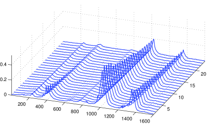
The NMR spectra are measured as intensity for each chemical shift (in the range 2.5–0.6ppm); see [4] for details. For each subject, a 2-D spectrum of dimensions $24\times 1600$ is produced, where the second dimension is the spectral one. The first dimension corresponds to 24 steps of gradient pulse strength. Figure 4 illustrates a typical example. Note that in this plot (and elsewhere) the spectral range is indexed sequentially from $1$; it does not show the true value chemical shift, since we did not have access to the exact value. In terms of dimension, this dataset lies between the in vivo and ex vivo fracture healing Raman datasets. It has both a spatial and a spectral dimension, making it a good fit for our modeling approach. Since the spectra are smooth along the spectral dimension, we have sub-sampled them at a rate $1/3$ as a preprocessing step to reduce the dimension of each spectrum to $534\times 24$.

3 Models and methods

In this section, we present our models for spectroscopy data, in general notation, but tailored to the in vivo Raman dataset of Section 2.1. We consider data that have one continuous (functional) dimension and several discrete (spatial) dimensions. In order to describe the model, we consider the case where there are two discrete dimensions and a single continuous one, although the results can be easily generalized. To be specific, the data is a collection

$$\big{\{}X_{ij}^{k}(\cdot):\,(i,j,k)\in[d]\times[p]\times[n]\big{\}}$$

of functions, recorded at spatial positions $(i,j)$. Here, we are using the notation $[p]:=\{1,\dots,p\}$ and similarly for $[d]$ and $[n]$. Index $k$ is used to enumerate the statistical samples. In other words,

$$\{X_{ij}^{1}(\cdot),\ (i,j)\in[d]\times[p]\},\;\{X_{ij}^{2}(\cdot),\ (i,j)\in[d]\times[p]\},\;\dots,\{X_{ij}^{n}(\cdot),\ (i,j)\in[d]\times[p]\}$$

are assumed to be i.i.d. samples in an experiment. We will use $t$ to denote the continuous index, and assume that each function $t\mapsto X_{ij}^{k}(t)$ is observed over some interval $T\subset\mathbb{R}$. Moreover, we refer to the continuous domain (i.e, $T$) as the spectral domain and to its elements (i.e., $t\in T$) as wavenumbers, based on our main application to in vivo Raman spectra, though the model is general. Similarly, we may refer to indices $i$ and $j$ as source and detector positions, respectively.

We consider two analysis goals involving this type of data. The first is that of finding an efficient (i.e., compact) and informative representation of the data. The second is that of using the relatively high-dimensional dataset $\{X_{ij}^{k}(t)\}$ as covariates in a regression problem to predict a response vector $\{y^{k}\}$. These goals are related, since obtaining a compact representation of the data greatly facilitates the regression analysis.

3.1 Functional representation

In order to obtain a compact representation of the data, we take each function $X_{ij}^{k}(\cdot)$ to lie in a reproducing kernel Hilbert space (RKHS) [1], generated by some kernel function $\mathbb{K}:T\times T\to\mathbb{R}_{+}$. Usually, the functions $\{X_{ij}^{k}(\cdot)\}$ are only observed at a discrete set of points $\mathcal{T}:=\{t_{1},t_{2},\dots,t_{N}\}$. We additionally assume that each $X_{ij}^{k}(\cdot)$ can be well approximated by a finite linear combination of the kernel functions anchored at points of $\mathcal{T}$. That is,

$$X_{ij}^{k}(t)\approx\sum_{v=1}^{N}x_{ijv}^{k}\;\mathbb{K}(t,t_{v}),\quad t\in T.$$ (1)

This assumption simplifies the subsequent derivations and is motivated (and somewhat justified) by the representer theorem [13]. The kernel function $\mathbb{K}$ can be taken to be any valid kernel (positive semi-definite, symmetric bivariate function), though our main focus will be on the Lorentzian

$$\mathbb{K}(t,s):=\frac{1}{1+(\frac{t-s}{W})^{2}},$$

where $W$ is a bandwidth parameter. Empirically, this kernel provides a good model for pure spectra, and is also justified by physical considerations [10]. Another restriction that we impose is for the coefficients $\{x_{ijv}^{k}\}$ to be nonnegative. This is also in accordance with the physics of how spectra are formed as a weighted linear combination of spectra of pure chemical components, without any cancellations.

Let us fix $(i,j,k)$ for the rest of this section. Based on (1), the idea is to turn the collection $\{X_{ij}^{k}(t)\}_{t\in T}$ into the set of coefficients $\{x_{ijv}^{k}\}_{v\in[N]}$, which is easier to work with. To achieve a compact representation, we impose a sparsity constraint on the vector $x_{ij\raisebox{-1.35623pt}{\scalebox{1.5}{$\cdot$}}}^{k}:=\{x_{ijv}^{k}\}_{v\in[N]}$. In other words, we seek a representation of the form (1) with as few nonzero coefficients as possible. This can be done by solving the $\ell_{1}$-regularized least-squares problem

$$\operatorname*{argmin}_{z\,\in\,\mathbb{R}^{N}_{+}}\Big{\{}\frac{1}{2}\sum_{u=1}^{N}\Big{[}X_{ij}^{k}(t_{u})-\sum_{v=1}^{N}z_{v}\;\mathbb{K}(t_{u},t_{v})\Big{]}^{2}+\lambda_{\mathcal{H}}\sum_{u,v=1}^{N}z_{u}z_{v}\mathbb{K}(t_{u},t_{v})+\lambda_{1}\sum_{v=1}^{N}|z_{v}|\Big{\}}.$$ (2)

Here, $\mathbb{R}^{N}_{+}$ is the set of $N$-vectors with nonnegative components. We note that the term $\sum_{u,v}z_{u}z_{v}\mathbb{K}(t_{u},t_{v})$ is the RKHS norm of the function $\sum_{v}z_{v}\mathbb{K}(\cdot,t_{v})$. When the RKHS norm measures smoothness of the function, regularizing by this term leads to smoother solutions.

Let $K$ be the $N\times N$ matrix with entries $\mathbb{K}(t_{u},t_{v})$, and let $\|z\|_{p}:=\big{(}\sum_{v=1}^{N}|z_{v}|^{p}\big{)}^{1/p}$ denote the $\ell_{p}$ norm of $z=(z_{1},z_{2},\dots,z_{N})$. Moreover, let $\bm{X}_{ij}^{k}:=\big{(}X_{ij}^{k}(t_{u})\big{)}_{u\in[N]}$ so that $\bm{X}_{ij}^{k}$ is an $N$-vector. Then, (2) can be rewritten in the compact form

$$\operatorname*{argmin}_{z\,\in\,\mathbb{R}^{N}_{+}}\Big{\{}\frac{1}{2}\|\bm{X}_{ij}^{k}-Kz\|_{2}^{2}+\lambda_{\mathcal{H}}\,z^{T}Kz+\lambda_{1}\|z\|_{1}\Big{\}}.$$ (3)

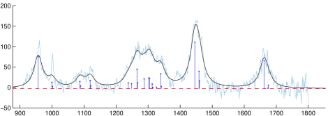
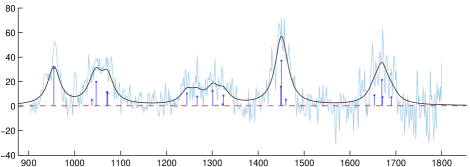
Note that this is a standard convex problem which can be solved efficiently. Figure 5 shows examples of fitted Raman spectra.

Figure 5: Examples of fitting model (1) to Raman spectra. The fitted spectra are shown in black; the estimated non-zero coefficients $\{x_{ijv}^{k}\}$ are shown as vertical lines, with height representing their magnitude.

3.2 Regression model

In this section we devise a model to predict a (one-dimensional) response vector $\{y^{k}\}$ based on the observed tensor covariates $\{X_{ij}^{k}(t)\}$. Perhaps the simplest model is to assume that a rank-one multilinear map relates the covariates to the response, that is, we consider the following regression model,

$$y^{k}=\sum_{ij}\int_{T}\alpha_{i}\beta_{j}w(t)\,X_{ij}^{k}(t)\,dt+\varepsilon^{k}$$ (4)

for $k=1,\dots,n$, where $\{\varepsilon^{k}\}$ are i.i.d. noise variables. In accordance with (1), we simplify the model further by assuming the following representation for $w$,

$$w(t):=\sum_{u=1}^{N}\gamma_{u}\mathbb{K}(t,t_{u}),\quad t\in T.$$ (5)

Combining with representation (1) for $\{X_{ij}^{k}(t)\}$ and ignoring its approximation error, we arrive at the model

$$y^{k}=\sum_{ijuv}\alpha_{i}\beta_{j}\gamma_{u}\,G_{uv}\,x_{ijv}^{k}+\varepsilon^{k}$$

where $G_{uv}:=\int_{T}\mathbb{K}(t,t_{u})\mathbb{K}(t,t_{v})\,dt$. Note that this is the $L^{2}(T)$ inner product of the functions $\mathbb{K}(\cdot,t_{u})$ and $\mathbb{K}(\cdot,t_{v})$. Let $G:=(G_{uv})\in\mathbb{R}^{N\times N}$, and note that this is a Gram matrix. The model can be written more compactly by defining

$$\widetilde{x}_{iju}^{k}:=\sum_{v=1}^{N}G_{uv}\,x_{ijv}^{k},\quad\text{so that}\quad y^{k}=\sum_{iju}\alpha_{i}\beta_{j}\gamma_{u}\,\widetilde{x}_{iju}^{k}+\varepsilon^{k},$$ (6)

where the summation is over $(i,j,u)\in[p]\times[d]\times[N]$. Note that the advantage of this rank-one model is that it contains $p+d+N$ variables, which in high dimensions is far less than that of a full linear model with $pdN$ variables.

In order to fit model (6), we again solve a regularized least-squares problem. Since $(i,j)$ represent spatial dimensions in our setting, we do not expect much sparsity in $\alpha=(\alpha_{i})$ and $\beta=(\beta_{j})$. Hence we use an $\ell_{2}$ norm regularizer for these two. On the other hand, we expect considerable sparsity in the spectral domain variable $\gamma=(\gamma_{u})$, hence we regularize by its $\ell_{1}$ norm.

The final element of our proposed regularizer is a penalty which tends to bring the coefficients assigned to nearby wavenumbers closer together. This is justified if proximity in the spectral domain signifies similarity, as suspected to be the case for Raman spectra. This type of regularizer also provides a practical advantage which is discussed in Section 3.3. As a measure of similarity between wavenumbers, we can use the Gram matrix $G$. It is then natural to use a weighted fused Lasso penalty [16, 2] of the form $\sum_{uv}G_{uv}|\gamma_{u}-\gamma_{v}|$.

Putting the pieces together, we solve the following

$$\begin{split}(\widehat{\alpha},\widehat{\beta},\widehat{\gamma})&=\operatorname*{argmin}_{\begin{subarray}{c}(\alpha,\,\beta,\,\gamma):\;\\ \alpha\,\geq\,0,\;\beta\,\geq\,0\end{subarray}}\Big{\{}\frac{1}{2n}\sum_{k=1}^{n}\Big{(}y^{k}-\sum_{iju}\alpha_{i}\beta_{j}\gamma_{u}\,\widetilde{x}_{iju}^{k}\Big{)}^{2}+\frac{\rho_{\alpha}}{\sqrt{p}}\,\|\alpha\|_{2}+\frac{\rho_{\beta}}{\sqrt{d}}\,\|\beta\|_{2}\\ &\qquad\qquad\qquad\qquad\qquad\qquad\qquad+\,\frac{\rho_{\gamma}}{N}\,\|\gamma\|_{1}+\frac{\rho_{G}}{N^{2}}\,\sum_{u,v=1}^{N}G_{uv}|\gamma_{u}-\gamma_{v}|\Big{\}}\end{split}$$ (7)

for some positive numbers $\rho_{\alpha},\rho_{\beta},\rho_{\gamma}$ and $\rho_{G}$. Conditions $\alpha\geq 0$ and $\beta\geq 0$ are interpreted element-wise. They are imposed to remove the sign-ambiguity which is otherwise present in the model. Note also that there is a general scale ambiguity in model (6), but not in (7) due to the presence of the regularizers. (By scale ambiguity, we mean that $(\alpha,\beta,\gamma)$ and $(c_{1}\alpha,c_{2}\beta,c_{2}\gamma)$ determine the same multilinear map as long as $c_{1}c_{2}c_{3}=1$ holds.)

Remark 1.

Enforcing an exact rank-one constraint on the regression function has been recently proposed in [19] in the context of regression with matrix covariates. Their model is similar to (4), without the functional dimension, i.e., $y^{k}=\sum_{ij}\alpha_{i}\beta_{j}X_{ij}^{k}+\varepsilon^{k}$. They enforce sparsity on both sets of coefficients $(\alpha)$ and $(\beta)$, using a multiplicative $\ell_{1}$ penalty. Our model provides an extension (with variation) to the tensor case with mixed functional and discrete dimensions. For us, the coefficients $(\alpha)$ and $(\beta)$ have physical (spatial) interpretations and are not necessarily sparse.

Remark 2.

Enforcing a low-rank assumption on the regression function, but not necessarily an exact one, has been studied extensively in recent years. The preferred approach to the problem is via nuclear norm penalization. We refer to [6, 11] for more details. Empirically, we found that imposing a rank-one assumption directly enhances the interpretation by considerably reducing the dimensionality. The drawback is the non-convexity of the resulting problem (see below) and lack of theoretical guarantees.

3.3 Practical considerations

Let us consider some practical issues regarding the models discussed earlier.

• The cost function in (7) is not (jointly) convex in $(\alpha,\beta,\gamma)$, but it is separately convex in each of these variables. A standard way to optimize such functions is by alternating minimization, fixing two variables at a time and minimizing over the other.

  

  

  Figure 6: Example of the scores obtained based on (8) for a sample of Raman data. The bottom plot shows the $40$ wavenmubers with the highest scores.

• In practice, we observe $\{X_{ij}^{k}(\cdot)\}$ at more points than we want to keep in the model. More specifically, we observe the functions at a set of points $\mathcal{T}^{\prime}\supset\mathcal{T}$, and we discard some of the points to obtain the $\mathcal{T}$ which is used in fitting the model. This is to avoid over-fitting. One approach to choose which points to keep is to assign a score to each point in $\mathcal{T}^{\prime}=\{t^{\prime}_{1},t^{\prime}_{2}\dots,t^{\prime}_{N^{\prime}}\}$, based on their weighted frequency of appearing in the dataset. For example, we can assign the following score to $t^{\prime}_{v}$,

  $$s_{v}:=\frac{1}{pdn}\sum_{ijk}x_{ijv}^{k},\quad v\in[N^{\prime}]$$ (8)

  where $\{x_{ijv}^{k}\}$ are the coefficients in expansion (1) of Section 3.2, and the sum runs for $(i,j,k)\in[p]\times[d]\times[n]$. We can then keep wavenumbers corresponding to the $N$ largest scores. Figure 6 shows the scores obtained for the example Raman data and the wavenumbers corresponding to $N=40$ largest scores. (Here $N^{\prime}=544$.)

• An advantage of the weighted fused Lasso penalty used in (7), in connection with the previous point, is that we do not need to worry about the order of the wavenumbers kept in $\mathcal{T}$. The Gram matrix $G$ automatically tries to match the coefficients of nearby wavenumbers regardless of how they are ordered in $\mathcal{T}$.

• It is possible to replace $\ell_{2}$ norm regularizations for $\alpha$ and $\beta$, with constraints $\sum_{i}\alpha_{i}=\sum_{i}\beta_{i}=1$. This gives $\alpha$ and $\beta$ the natural interpretation of being probability vectors. We have not used this version here, since it tends to have a similar effect as an $\ell_{1}$ regularization (note that $\alpha,\beta\geq 0$), that is, it produces sparse solutions. It is more suitable in situations in which only few of the spatial positions are suspected to be influential, which is not the case for data considered here.

• In practice, we choose the regularization parameters in both (3) and (7) by cross-validation (CV). The scaling of regularization parameters in (7) by $1/\sqrt{p}$, $1/\sqrt{d}$, etc. is to keep the corresponding parameters in the same range, and have little effect in practice if CV is used.

• Although the model (4) is designed to pick the correct normalization constants for each source-detector combination, through $(\alpha)$ and $(\beta)$, in practice some form of crude scaling is useful prior to fitting the model, to keep all the waveforms on a reasonable scale. We consider two simple approaches, each of which can be applied to either $\{x_{ijv}^{k}\}$ or $\{\widetilde{x}_{iju}^{k}\}$. These are specific to the in vivo Raman application, for which $(i,j)$ refers to source-detector position. Other approaches might be suitable in different applications.

  The first approach is to normalize, e.g., $\{\widetilde{x}_{iju}^{k}\}$ so that the maximum amplitude among all the data for a particular source-detector combination is $1$. That is, we work with the normalized sequence $\{\widetilde{x}_{iju}^{k}/(\max_{k,u}\widetilde{x}_{iju}^{k})\}$. The other approach is to normalize so that the total energy (in the sense of $\ell^{2}$-norm) corresponding to each source position is unit, in each application of the measuring device (i.e., for each $k$). More specifically, we look at the rescaled sequence $\big{\{}x_{ijv}^{k}/\sqrt{\sum_{jv}(x_{ijv}^{k})^{2}}\big{\}}$. A more elaborate version of this normalization could take into account the kernels anchored at each wavenumber and use the continuous $L^{2}$ norm.

  Empirically, the two approaches outlined above produce comparable results. For definiteness, the results reported in the Section 4 are based on the maximum amplitude normalization (unless otherwise stated).

4 Empirical results

4.1 In vivo Raman

We start by applying the models of Section 3 to the in vivo Raman data. Here, the models are applicable verbatim. To obtain the results, we have centered the BMD sequence $\{y^{k}\}$ and normalized so that its maximum absolute value is equal to $1$, that is, $\frac{1}{n}\sum_{k}y_{k}=0$ and $\max_{k}|y_{k}|=1$. The modified Raman tensor $\{\widetilde{x}_{iju}^{k}\}$ is normalized according to the first approach discussed in Section 3.3, so as to have the maximum amplitude of $1$ for every source-detector pair.

Figure 7: Normalized BMD estimation. The plots show examples of estimated versus observed normalized BMD for the training (blue) and prediction (red) sets. The six plots correspond to six random splittings of the data into training and prediction sets.

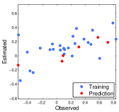
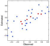
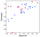
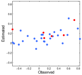
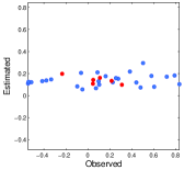
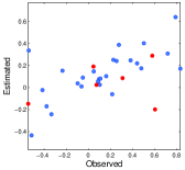
Figure 7 shows some examples of predictive performance of the regression model (6). In each case, the sample is split randomly into a training set and a test set, the latter containing 2 rats from each of weeks 4, 6 and 8. We have also discarded 5 rats from the sample as outliers, based on their average prediction error across all the partitions – for those five, the average prediction errors were significantly higher than the rest. We refer to each such partition of the data as a cross-validation or CV batch. Thus, each CV batch contains 26 training and 6 test rats. A total of $50$ CV batches were considered. For each batch, we have chosen the regularization parameters to minimize the prediction error on the test set. We will call this the adaptive (or oracle) choice for the parameters. This gives the best performance we could hope that the model achieves in each case. It can be seen the results are mixed, even with this optimal choice of the parameters, with some partitions of the data allowing for a good prediction and some not.

Adaptive Regularization

Fixed Regularization

Figure 8: Relative prediction performance. The plots show the mean absolute deviation error, in normalized BMD estimation, for the training (blue) and prediction (red) sets of our proposed regression model (6), versus the error of prediction by the mean. Also shown (green) is the error of the simpler ratio regression approach. The two panels correspond to the adaptive versus fixed choice of regularization parameters in regression model (6).

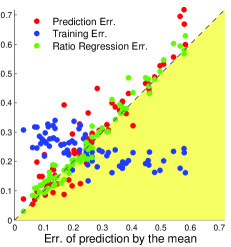
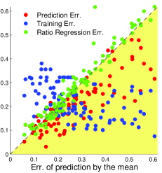
The left panel of Figure 8 illustrates the same setting, but from the perspective of prediction errors. We have used the median absolute deviation (MAD) as our measure of performance (which will be the default throughout). The $x$-axis on this plot shows the error of the prediction by the mean, by which we mean the error of the estimator that outputs the mean of the training set (which is $\approx 0$) disregarding the Raman data. We will use the error of this constant estimator as a baseline. The $y$-axis shows the training error, and the test error of our model, together with the test error of a simpler approach which we have called ratio regression, to be described shortly. Each point in this plot corresponds to a CV batch. Each point below the diagonal line shows a partition of the data that can be predicted better by the model than the baseline. With the adaptive choice of the regularizer, this holds for almost all the batches.

The ratio regression approach predicts the BMD by regressing against a simple spectral feature, namely the ratio of two peaks of interest, at wavenumbers $954\text{\,}\mathrm{c}\mathrm{m}^{-1}$ and $1450\text{\,}\mathrm{c}\mathrm{m}^{-1}$, which are known to correspond to mineral (calcuim) and matrix (collagen), respectively. The higher the ratio, the higher is the likelihood of the bone being present in the specimen, as suspected by the chemists. The average of these two peaks (across all source-detector positions) is computed for each rat, the mineral-to-matrix ratio is computed by dividing the amplitude of $954\text{\,}\mathrm{c}\mathrm{m}^{-1}$ peak to that of $1450\text{\,}\mathrm{c}\mathrm{m}^{-1}$, and the result is used as the covariate to predict the BMD. This method, or a version of it, is typically used by Raman spectroscopists. Figure 8 shows that the result is very similar to the baseline of predicting by the mean, meaning using Raman spectra in this fashion does not help predict BMD in this experiment.

The right panel of Figure 8 shows the results for a more standard choice of the regularization parameters which we have called fixed regularization. In this case, a fixed set of parameters is used for all batches, and they are chosen so that the average error over all batches (i.e., the CV error) is minimized. With this choice it can be seen that the performance of our model is similar to that of ratio regression and the baseline).

We draw three main conclusions from these results. First, predicting BMD (or similar measures) from in vivo Raman is inherently difficult, as is suggested by the fact that both the simple ratio regression and our more elaborate model with fixed regularization fail to show significant improvement over the mean. This may be partly due to the mixing of bone and tissue signals, partly due to variability in the rats and the small sample size, and partly due to the quality of the Raman data from this experiment. Second, the fact that we can successfully predict for some batches and not for the others suggests that the rats are not homogeneous; if we had enough samples from each (latent) group of similar rats, we might be able to improve the prediction. Finally, we suspect that the present dataset might have been plagued by some calibration (or systematic) errors, which precludes a global improvement on prediction performance. This is suggested by the poor performance of the ratio regression, which is believed to be a reasonably effective marker of healing. Figure 10 below also reinforces this point. In other words, only in situations where ratio regression shows some improvement over the mean, we can hope and expect that our method provides further improvements. The ex vivo results to be discussed below support this claim.

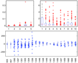
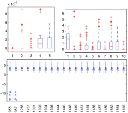
Figure 9 shows the estimated coefficients of the model. The three sets of coefficients are the $5$-vector of source weights ($\alpha$), the $10$-vector of detector weights ($\beta$) and the $40$-vector of wavenumber weights ($\gamma$). The high number of outliers in source/detector weights and the general tendency of the wavenumber weights to fluctuate around zero are in alignment with conclusions above, that is, no global correlation between this dataset and BMD can be inferred.

Adaptive Regularization

Fixed Regularization

Figure 9: Estimated model coefficients for the in vivo dataset, for both adaptive and fixed regularization. Boxplots of source weights ($5$-vector), detector weights ($10$-vector) and wavenumber weights ($40$-vector) are illustrated.

Figure 10: Piecewise-constant approximation to regression curves for peaks of interest. Form left to right the plots show the normalized (and centered) scores obtained for $954\text{\,}\mathrm{c}\mathrm{m}^{-1}$ and $1450\text{\,}\mathrm{c}\mathrm{m}^{-1}$ wavenumbers and their ratio, versus the normalized BMD. The range of BMD is divided into three bands, and the mean (dark red) and the median (light red) of scores within each band are shown. The points are color-coded based on the week they belong to, with week 4, 6 and 8 being light, moderate and dark green, respectively.

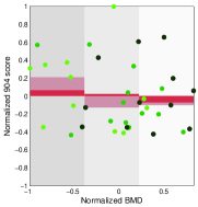
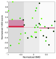
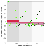
We conclude this section with another look at the in vivo dataset from the perspective of ratio regression. Figure 10 illustrates scatter plots for the two peaks of interest, at $954$ and $1450\text{\,}\mathrm{c}\mathrm{m}^{-1}$, and their ratios, versus the (normalized) BMD. The values for the peaks are those obtained from our functional representation , and are centered and normalized to maximum absolute value $1$.

The range of BMD is divided into three bands and the mean and median of the $y$-axis data is shown in each band. This provides a piecewise-constant approximation to the regression curve. These plots show the somewhat anomalous nature of the dataset. We would expect that as ossification progresses (BMD increases) the calcium-related $954\text{\,}\mathrm{c}\mathrm{m}^{-1}$ should increase, while the collagen-related $1450\text{\,}\mathrm{c}\mathrm{m}^{-1}$ should decrease. A near reversal of this trend is observed for the mean behavior of $954\text{\,}\mathrm{c}\mathrm{m}^{-1}$, while the $1450\text{\,}\mathrm{c}\mathrm{m}^{-1}$ follows the expected relationship to some extent. As a result, their ratio remains almost constant, on average, over the entire range of BMD (with a slight deviation towards the lower end), preventing a possible prediction. This further reinforces our suspicion of a calibration error; getting the ring aligned with exact location of the defect is, in general, difficult. The current version of the ring also was not in contact with the leg. Thus, slight variations in its position might have caused nearby healthy bone to contribute to the spectra. (More precise construction of the ring has been proposed and is under investigation.)

4.2 Ex vivo Raman

For ex vivo data of Section 2.2, there is no spatial dynamics to be modeled. That is, $p=d=1$, and the model reduces to a more or less classical functional regression with Lasso and fused Lasso penalties. In this case, we only have one set of parameters to estimate, namely, $\{\gamma_{u}\}$ or equivalently, the functional weights $w(t)$ of (5).

Cross-validation Errors

Estimated Coefficients

Figure 11: The results for ex vivo dataset. Left panel shows, from left to right, CV errors for the baseline (prediction by the mean), prediction error for our model followed by its training error, and the error of ratio regression. Right panel shows the estimated model coefficients.

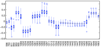
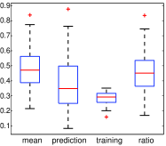
Figure 11 (left panel) shows cross-validation (CV) errors for our model (in both prediction and training) versus the baseline (prediction by the mean) and ratio regression. The latter two are as described in the context of in vivo data (cf. Section 4.1). Here, the parameters of our model are set by CV in the usual sense; that is, a fixed set of parameters are used for all the batches, chosen so that average CV error is minimized. The partitioning of data into prediction and training sets, and the number of batches are as in Section 4.1. One observes that our model provides a fair improvement (on average) over the simpler ratio regression which is only slightly better than the baseline.

Also shown in Figure 11 (right panel) are the boxplots of the estimated coefficients $\{\gamma_{u}\}$. In contrast to the in vivo case, one can clearly identify regions (wavenumbers) that consistently exhibit large coefficients and hence are helpful in predicting the BMD. For example, the mineral band at $\approx 954$ (which is known to be excited by calcium in the bone) is prominent in the plot. Another interesting observation is that of the two collagen bands, one at $\approx$1450\text{\,}\mathrm{c}\mathrm{m}^{-1}$$ and the other at $\approx$1660\text{\,}\mathrm{c}\mathrm{m}^{-1}$$, the latter seems to be more correlated with BMD, despite the fact that $1450\text{\,}\mathrm{c}\mathrm{m}^{-1}$ is in general the highest amplitude peak in the Raman spectra (cf. Figure 5). Overall, these results suggest that the main challenges in using Raman spectra to predict BMD come from the attempt to do it in vivo, rather than some inherent problem with the bone spectra themselves.

4.3 NMR

The regression model introduced in 3.2 has two spatial dimensions, which is one more than what is needed for the NMR dataset; we discard one dimension by setting, say, $d=1$. Then, the model has two sets of parameters to be estimated, $\{\alpha_{i}\}$ and $\{\gamma_{u}\}$. As with the Raman datasets, we retain the $N=40$ highest scoring chemical shifts in the model.

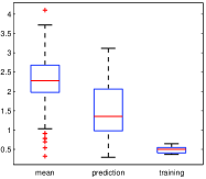
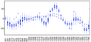
Figure 12 shows cross-validation (CV) results for the NMR dataset. A total of 50 batches were used for CV, where in each batch we left 4 samples out for prediction (out of a total of $n=20$). The left panel in the figure shows CV errors for the baseline (prediction by the mean) and for our model (both prediction and training errors). We observe a substantial improvement by our model over the baseline. The left panel shows the boxplots for estimated coefficients $\alpha$ (on the top) and $\gamma$ (on the bottom). These clearly show some spatial and spectral positions to predict the response. It further illustrates that with a sufficiently high signal-to-noise ratio, our models can be used for prediction and variable selection.

Cross-validation Errors

Estimated Coefficients ($\alpha,\gamma$)

Figure 12: The results for NMR dataset. Left panel shows, from left to right, CV errors for the baseline (prediction by the mean), and prediction error for our model followed by its training error. Right panel shows the estimated model coefficients.

5 Discussion

We presented a functional model for spectra which can be used for denoising and compression. Based on this representation of the data, we proposed a regression model to predict a scalar response (e.g., bone mineral density or lipoprotein concentration) based on multi-dimensional spectroscopy data. The data was modeled as a tensor with several spatial dimensions and one spectral dimension. A rank-one multilinear map was proposed to describe the relation between the spectra and the response, with some structure on the coefficients, namely sparsity in the spectral domain, and dependence based on a similarity measure. The structure was enforced using regularization, with $\ell_{1}$ penalty to induce sparsity, and a fused Lasso type penalty to enforce similarity. (Some structure was also assumed for the spatial coefficients, albeit a minimal one.)

We considered the effectiveness of the approach in three settings: in vivo and ex vivo Raman data from a fracture healing experiment, and using NMR data in a lipoprotein concentration study. For the in vivo Raman experiments, our results were mixed. It was possible to predict the outcome for some partitions of the data into training and prediction sets, but not for others. Overall our model and a simpler ratio regression model suggested that there was no significant global relation between the in vivo Raman data at hand and the BMD outcome. We conjectured three possible causes: (1) The problem of prediction based on in vivo Raman data is hard in general, due to bone-tissue mixing, low signal-to-noise ratio and normalization issues. (2) The prediction is possible for a more homogeneous group of rats than what we had. This was suggested by good results if we used adaptive regularization (i.e., picked the best choice for each batch of CV). (3) The data at hand may have been corrupted by calibration and systematic errors. This was further corroborated by looking at piecewise constant approximations to regression curve for predicting BMD based on single peaks in the spectra, which are known to correlate with bone composition. This issue is partly due to the difficulty of aligning the measuring device with the exact location of the fracture, which is a known challenge that is under investigation. For the ex vivo Raman data, and the NMR, we showed that the model has (global) predictive power, and can improve significantly over the baseline of prediction by the mean.

In this paper we mainly focused on regression models. Another interesting possibility for future work is to look at PCA type analyses, by which we mean models taking into account a decomposition of the spectra into relevant (and irrelevant) components. A promising direction is to use the response variable to guide the selection of components. Another feature of the problem, namely the positivity of spectra, can also be taken into account, which makes the problem different from classical PCA, or PCA-based regression. A challenge in this case is to find alternatives to orthogonality which are meaningful for positive components.

References

- [1] A Berlinet and C Thomas-Agnan. Reproducing Kernel Hilbert Spaces in Probability and Statistics. Springer US, Boston, MA, 2004.
- [2] X Chen, Q Lin, and S Kim. Smoothing proximal gradient method for general structured sparse regression. The Annals of Applied Statistics, 6(2):719–752, June 2012.
- [3] W Chew, E Widjaja, and M Garland. Band-Target Entropy Minimization (BTEM): An Advanced Method for Recovering Unknown Pure Component Spectra. Application to the FTIR Spectra of Unstable Organometallic Mixtures. Organometallics, 21(9):1982–1990, April 2002.
- [4] M Dyrby, M Petersen, A K Whittaker, L Lambert, L Nörgaard, Rasmus Bro, and Søren Balling Engelsen. Analysis of lipoproteins using 2D diffusion-edited NMR spectroscopy and multi-way chemometrics. Analytica Chimica Acta, 531(2):209–216, February 2005.
- [5] E B Hanlon, R Manoharan, T W Koo, K E Shafer, J T Motz, M Fitzmaurice, J R Kramer, I Itzkan, R R Dasari, and M S Feld. Prospects for in vivo Raman spectroscopy. Physics in medicine and biology, 45(2):R1–59, February 2000.
- [6] V Koltchinskii, K Lounici, and A B Tsybakov. Nuclear-norm penalization and optimal rates for noisy low-rank matrix completion. The Annals of Statistics, 39(5):2302–2329, October 2011.
- [7] J R Maher, J A Inzana, H A Awad, and A J Berger. Overconstrained library-based fitting method reveals age- and disease-related differences in transcutaneous Raman spectra of murine bones. Journal of biomedical optics, 18(7):077001, July 2013.
- [8] A A Martin, R A Bitar Carter, L de Oliveira Nunes, E A Loschiavo Arisawa, and L Silveira, Jr. Principal components analysis of FT-Raman spectra of ex vivo basal cell carcinoma. In SPIE 5321, Biomedical Vibrational Spectroscopy and Biohazard Detection Technologies, volume 5321, pages 198–204, July 2004.
- [9] P Matousek, E R C Draper, A E Goodship, I P Clark, K L Ronayne, and Anthony W Parker. Noninvasive Raman spectroscopy of human tissue in vivo. Applied spectroscopy, 60(7):758–63, July 2006.
- [10] R J Meier. On art and science in curve-fitting vibrational spectra. Vibrational Spectroscopy, 39(2):266–269, October 2005.
- [11] S Negahban and M J Wainwright. Estimation of (near) low-rank matrices with noise and high-dimensional scaling. The Annals of Statistics, 39(2):1069–1097, April 2011.
- [12] V P Pauca, J Piper, and R J Plemmons. Nonnegative matrix factorization for spectral data analysis. Linear Algebra and its Applications, 416(1):29–47, July 2006.
- [13] B Schölkopf, R Herbrich, and A J Smola. A generalized representer theorem. Computational learning theory, pages 416–426, 2001.
- [14] C N Tchanque-Fossuo, B Gong, B Poushanchi, A Donneys, D Sarhaddi, K Kelly Gallagher, Sagar S Deshpande, Steven a Goldstein, Michael D Morris, and Steven R Buchman. Raman spectroscopy demonstrates Amifostine induced preservation of bone mineralization patterns in the irradiated murine mandible. Bone, 52(2):712–7, February 2013.
- [15] R Tibshirani. Regression shrinkage and selection via the lasso. Journal of the Royal Statistical Society. Series B, 58(1):267–288, 1996.
- [16] R Tibshirani, M Saunders, S Rosset, J Zhu, and K Knight. Sparsity and smoothness via the fused lasso. Journal of the Royal Statistical Society: Series B, 67(1):91–108, February 2005.
- [17] V Vrabie, C Gobinet, O Piot, A Tfayli, P Bernard, Régis Huez, and Michel Manfait. Independent component analysis of Raman spectra: Application on paraffin-embedded skin biopsies. Biomedical Signal Processing and Control, 2(1):40–50, January 2007.
- [18] Effendi Widjaja, Nicole Crane, Tso-Ching Chen, Michael D Morris, Michael A Ignelzi, and Barbara R McCreadie. Band-target entropy minimization (BTEM) applied to hyperspectral Raman image data. Applied spectroscopy, 57(11):1353–62, November 2003.
- [19] J Zhao and C Leng. Structured Lasso for Regression with Matrix Covariates. Statistica Sinica, To appear, 2013.