Guided modes in a spatially dispersive wire medium slab

Abstract

We study the guided modes in the wire medium slab taking into account both the nonlocality and losses in the structure. We show that due to the fact that the wire medium is an extremeley spatially dispersive metamaterial, the effect of nonlocality plays a critical role since it results in coupling between the otherwise orthogonal guided modes. We observe both the effects of strong and weak coupling, depending on the level of losses in the system.

I Introduction

Wire metamaterials have a number of unique properties wirereview , including the possibility of the subwavelength image transfer Subwavelength1 ; Subwavelength2 ; Subwavelength3 , negative refraction negrefr and spontaneous emission time engineering polar . Localized modes in the slabs of wire metamaterial have been studied previously in a number of papers Theor ; Belovmodes , and it was shown that these modes are similar to the so-called spoof plasmons, a special class of surface modes, which propagate along corrugated metal or semiconductor surfaces spoof001 ; spoof01 ; spoof . Furthermore, it has been shown that the excitation of the guided modes in the wire metamaterial slab is critical for the realization of the far-field superlensing FinkPRL ; Finkfirst .

While the guided waves in the wire metamaterial slab have been studied previously Finkwaveguides ; FinkWCM , there are no consistent studies of these modes that simultaneously account for the three distinctive features of these structures: the spatial dispersion of the dielectric permittivity (arising from the nonlocality of the wire medium’s response to electromagnetic field), the presence of the wire host medium with dielectric permittivity different from that in vacuum, and the presence of the inevitable losses. At the same time, such an analysis is currently extremely demanded, since the realizations of the wire medium at the moment exist for a wide range of frequencies spanning from microwave to the optical range, and both spatial dispersion and essential losses are present in these samples. Thus, in order to correctly describe the effects being observed experimentally in the existing wire media samples, these features should be taken into account.

In this work, we present a consistent analysis of the properties of the guided waves in the wire metamaterial slabs, which accounts for all aforementioned effects. We present two approaches to obtaining the dispresion equations for the eigenmodes of the waveguiding metamaterial slabs, both yielding the same results. We then analyze the obtained band structure of the symmetric and antisymmetric eigenmodes of the waveguide. We start from recalling the results for the local case (when the dielectric permittivity of the metamaterial at a given position is assumed to be a function of that position only), and then compare with the obtained results for the nonlocal approach (when the dielectric permittivity at a given position is a function of both that position and its neighborhood). We find, in particular, that the nonlocal effects lead to a strong coupling between “fast” and “slow” eigenmodes of the waveguide, manifested by anti-crossings of their dispersion curves. We also study how the losses in the host media affect the dispersion and the coupling of the guided modes.

The paper is organized as follows: in section II.1 we present the detailed problem setup; in section II.2 general impedance relations at the boundary of wire media slab are derived; section II.3 is dedicated to the derivation of the dispersion equation for the symmetric and antisymmetric guided modes; band structures of the eigenmodes are presented in section III.1 and the profiles of the electric fields for different eigenmodes are presented in III.2. In section III.3 it is shown how the losses in the structure affect the dispersion properties of the eigenmodes, and the conclusions are presented in section IV.

II Guided modes in a homogenized wire medium slab

II.1 Problem setup

We consider a planar slab of wire medium (WM), composed of ideally conducting parallel thin wires (oriented perpendicular to the slab surfaces), which are embedded in a uniform host medium with a constant dielectric permittivity $\varepsilon_{h}$. The slab has a thickness $a$, occupying the region $0\leq x\leq a$, and is cladded on both sides by a dielectric with a constant dielectric permittivity $\varepsilon_{d}$, as shown in Fig. 1.

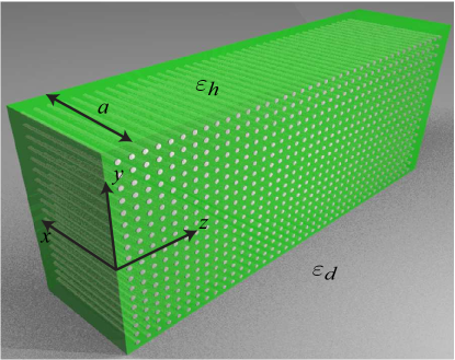
Figure 1: Waveguiding structure: a planar slab of wire medium of thickness $a$, cladded on both sides by a uniform dielectric with a constant permittivity $\varepsilon_{d}$. The wire medium consists of parallel perfectly conducting wires embedded into a uniform host medium with a dielectric permittivity $\varepsilon_{h}$.

We are interested in guided electromagnetic modes of such structure, with wavelengths that are large compared to the largest characteristic spatial scale of the wire medium (the latter is the period of the wire array in WM). Under such conditions, the bulk wire medium can be described as a uniaxial spatially dispersive (nonlocal) medium with an effective dielectric permittivity tensor Belov_etal_PRB_2003 ; Maslovski_PRB_2009 (we use SI units throughout)

$$\boldsymbol{\varepsilon}_{\rm WM}=\varepsilon_{0}\varepsilon_{h}\left(\varepsilon_{xx}(\omega,k_{x})\ \mathbf{\hat{x}}\mathbf{\hat{x}}+\mathbf{\hat{y}}\mathbf{\hat{y}}+\mathbf{\hat{z}}\mathbf{\hat{z}}\right),$$ (1)

with

$$\varepsilon_{xx}(\omega,k_{x})=1-\frac{\omega_{h0}^{2}}{\omega^{2}-c_{h}^{2}k_{x}^{2}},$$ (2)

where $c_{h}=c/\sqrt{\varepsilon_{h}}$ is the speed of light in the host medium of the WM (we assume a non-magnetic host medium with $\mu_{h}=1$), $\omega_{h0}=\omega_{p}/\sqrt{\varepsilon_{h}}$, $\omega_{p}=ck_{p}$ is the “plasma frequency” of the WM with $k_{p}$ defined in Eq. (10) of Belov_etal_PRB_2003 , $k_{x}$ is the $\mathbf{k}$-vector component along the wires, $c$ is the speed of light in vacuum, and $\omega$ and $\mathbf{k}$ are the frequency and wavevector of a Fourier-transformed electromagnetic field associated with the electromagnetic modes of the unbounded WM.

We consider electromagnetic waves propagating along the WM slab; choosing axis $z$ along the direction of propagation, we have, without reducing generality of the problem, the following structure of the electromagnetic waves propagating in the considered structure:

$$\{\mathbf{E,B}\}=\{\mathbf{E}(x),\mathbf{B}(x)\}e^{i\left(\omega t-k_{z}z\right)}.$$

We note that, since the WM dielectric tensor (1) is invariant with respect to rotations of coordinate frame around axis $x$ (which is fixed by assuming that the wires are perpendicular to the slab boundaries), its form remains the same as (1) in the chosen coordinate frame with axis $z$ directed along the direction of propagation of the guided modes.

Writing the Maxwell’s equations for $\mathbf{E,B}$ and applying Fourier transforms with respect to $t$ and $z$ (but not $x$), we obtain the following set of equations for the components of Fourier-transformed fields $\mathbf{E}^{(\omega,k_{z})}(x)$ and $\mathbf{B}^{(\omega,k_{z})}(x)$:

$$i\omega B_{x}^{(\omega,k_{z})} = -ik_{z}E_{y}^{(\omega,k_{z})},$$

$$i\omega B_{y}^{(\omega,k_{z})} = ik_{z}E_{x}^{(\omega,k_{z})}-\frac{\partial E_{z}^{(\omega,k_{z})}}{\partial x},$$

$$i\omega B_{z}^{(\omega,k_{z})} = \frac{\partial E_{y}^{(\omega,k_{z})}}{\partial x},$$

$$-c^{2}\varepsilon_{0}ik_{z}B_{y}^{(\omega,k_{z})} = -i\omega\varepsilon_{0}E_{x}^{(\omega,k_{z})}+j_{x}^{(\omega,k_{z})},$$

$$c^{2}\varepsilon_{0}ik_{z}B_{x}^{(\omega,k_{z})}-c^{2}\varepsilon_{0}\frac{\partial B_{z}^{(\omega,k_{z})}}{\partial x} = -i\omega\varepsilon_{0}E_{y}^{(\omega,k_{z})}+j_{y}^{(\omega,k_{z})},$$

$$c^{2}\varepsilon_{0}\frac{\partial B_{y}^{(\omega,k_{z})}}{\partial x} = -i\omega\varepsilon_{0}E_{z}^{(\omega,k_{z})}+j_{z}^{(\omega,k_{z})},$$ (3)

where $j_{x,y,z}^{(\omega,k_{z})}$ are the components of the Fourier-transformed (with respect to $t$ and $z$) effective current $\mathbf{j}(t,\mathbf{r})$ in the corresponding medium (either WM or a cladding dielectric in our case), defined by the constitutive relations of the medium. Thus Eqs (3) with the corresponding effective current densities are valid both in WM (at $0\leq x\leq a$) and in the cladding dielectric ($x<0$ and $x>a$).

It can be easily seen that in a bulk WM with dielectric tensor (1), as well as in a cladding dielectric with a constant $\varepsilon_{d}$, one has $j_{i}^{(\omega,k_{z})}\propto E_{i}^{(\omega,k_{z})}$, with index $i=x,y,z$. Therefore, Eqs (3) separate into two independent sets of equations for $E_{x},E_{z},B_{y}$ (TM wave) and $E_{y},B_{x},B_{z}$ (TE wave). Below we consider guided TM modes of the structure.

II.2 Guided TM modes

For TM modes, the relevant equations from the complete set (3) are

$$ik_{z}E_{x}^{(\omega,k_{z})}-\frac{\partial E_{z}^{(\omega,k_{z})}}{\partial x}-i\omega B_{y}^{(\omega,k_{z})} = 0,$$

$$c^{2}\varepsilon_{0}ik_{z}B_{y}^{(\omega,k_{z})}-i\omega\varepsilon_{0}E_{x}^{(\omega,k_{z})}+j_{x}^{(\omega,k_{z})} = 0,$$

$$c^{2}\varepsilon_{0}\frac{\partial B_{y}^{(\omega,k_{z})}}{\partial x}+i\omega\varepsilon_{0}E_{z}^{(\omega,k_{z})}-j_{z}^{(\omega,k_{z})} = 0.$$ (4)

The boundary conditions for Eqs (4) follow from (i) continuity of tangential field components $E_{z}$ and $B_{y}$, and (ii) arrest of the normal component $j_{x}$ of the effective WM current density at the slab boundaries $x=0,a$.

We solve Eqs (4) in the wire medium ($0\leq x\leq a$) using Fourier method; see Appendix A for details. As a result, we obtain the impedance relations between the tangential components of electric and magnetic fields at the WM slab boundaries $x=0,a$:

$$E_{z}^{(\omega,k_{z})}(0)=-iS_{1}B_{y}^{(\omega,k_{z})}(0)+iS_{2}B_{y}^{(\omega,k_{z})}(a),$$ (5)

$$E_{z}^{(\omega,k_{z})}(a)=-iS_{2}B_{y}^{(\omega,k_{z})}(0)+iS_{1}B_{y}^{(\omega,k_{z})}(a),$$ (6)

with

$$S_{1} = \frac{2c^{2}}{\omega\varepsilon_{h}a}\left.\sum_{n=0}^{\infty}\right.^{\prime}{\frac{c^{2}k_{z}^{2}-\omega^{2}\varepsilon_{h}\varepsilon_{xx}(n)}{c^{2}k_{z}^{2}-\omega^{2}\varepsilon_{h}\varepsilon_{xx}(n)+c^{2}\alpha_{n}^{2}\varepsilon_{xx}(n)}},$$ (7)

$$S_{2} = \frac{2c^{2}}{\omega\varepsilon_{h}a}\left.\sum_{n=0}^{\infty}\right.^{\prime}{(-1)^{n}\frac{c^{2}k_{z}^{2}-\omega^{2}\varepsilon_{h}\varepsilon_{xx}(n)}{c^{2}k_{z}^{2}-\omega^{2}\varepsilon_{h}\varepsilon_{xx}(n)+c^{2}\alpha_{n}^{2}\varepsilon_{xx}(n)}},$$ (8)

where $\varepsilon_{xx}(n)=\varepsilon_{xx}(\omega,k_{x}=\alpha_{n})$, and $\alpha_{n}=n\pi/a$. Below we consider the impedance relations for nonlocal and local models of wire medium slabs.

II.2.1 Nonlocal wire medium slab

Substituting $\varepsilon_{xx}(n)$, corresponding to the spatially dispersive model of WM with the nonlocal response (2), into (7)–(8), introducing dimensionless variables $\Omega=\omega/\omega_{h0}$, $K_{z}=ck_{z}/\omega_{h0}$, $\tilde{\alpha}_{n}=n\pi/\tilde{a}$, $\tilde{a}=(\omega_{h0}/c)a$, and carrying out the summation, we obtain the impedance relations for a nonlocal WM slab model:

$$S_{1}=S_{1}^{\rm nl} = \frac{c}{\varepsilon_{h}\Omega}\frac{1}{K_{z}^{2}+\varepsilon_{h}}\left[\frac{\varepsilon_{h}^{3/2}\Omega}{\tan\left(\tilde{a}\varepsilon_{h}^{1/2}\Omega\right)}+\frac{K_{z}^{2}\kappa_{x}}{\tanh\left(\tilde{a}\kappa_{x}\right)}\right],$$ (9)

$$S_{2}=S_{2}^{\rm nl} = \frac{c}{\varepsilon_{h}\Omega}\frac{1}{K_{z}^{2}+\varepsilon_{h}}\left[\frac{\varepsilon_{h}^{3/2}\Omega}{\sin\left(\tilde{a}\varepsilon_{h}^{1/2}\Omega\right)}+\frac{K_{z}^{2}\kappa_{x}}{\sinh\left(\tilde{a}\kappa_{x}\right)}\right],$$ (10)

where $\kappa_{x}=\sqrt{K_{z}^{2}-\varepsilon_{h}\left(\Omega^{2}-1\right)}$.

II.2.2 Local wire medium slab

A local model of the WM slab was proposed in Luukkonen_etal_2008 as a quasi-static approximation of the uniaxial wire medium considered here, with the nonlocal $\varepsilon_{xx}$ of (2) replaced by its local approximation

$$\varepsilon_{xx}^{\rm l}=1-\frac{\omega_{h0}^{2}}{\omega^{2}}.$$ (11)

With (11) substituted into (7)–(8), we obtain the impedance relations for a local WM slab model (i.e., with the spatial dispersion ignored):

$$S_{1}=S_{1}^{\rm l} = \frac{c}{\varepsilon_{h}\sqrt{\Omega^{2}-1}}\frac{\kappa_{x}}{\tanh\left(\frac{\Omega}{\sqrt{\Omega^{2}-1}}\tilde{a}\kappa_{x}\right)},$$ (12)

$$S_{2}=S_{2}^{\rm l} = \frac{c}{\varepsilon_{h}\sqrt{\Omega^{2}-1}}\frac{\kappa_{x}}{\sinh\left(\frac{\Omega}{\sqrt{\Omega^{2}-1}}\tilde{a}\kappa_{x}\right)},$$ (13)

where again $\kappa_{x}=\sqrt{K_{z}^{2}-\varepsilon_{h}\left(\Omega^{2}-1\right)}$.

The obtained impedance relations (9)–(10) and (12)–(13) for nonlocal and local WM slabs, respectively, together with the impedances of both semi-bounded dielectrics cladding the slab, allow to find the dispersion relations for guided modes of such slabs. Below we consider symmetric and antisymmetric TM modes of both nonlocal and local WM slabs.

II.3 Dispersion equations for symmetric and antisymmetric TM modes

There are two types of modes that can propagate in the WM slab: symmetric and antisymmetric. In a symmetric TM wave the tangential electric field $E_{z}^{\omega,k_{z}}(x)$ is symmetric, and the tangential magnetic field $B_{y}^{\omega,k_{z}}(x)$ is antisymmetric with respect to the WM slab mid-plane:

$$E_{z}^{\omega,k_{z}}(0)=E_{z}^{\omega,k_{z}}(a);\ \ B_{y}^{\omega,k_{z}}(0)=-B_{y}^{\omega,k_{z}}(a).$$

Conversely, in an antisymmetric TM wave the tangential electric field $E_{z}^{\omega,k_{z}}(x)$ is antisymmetric, and the tangential magnetic field $B_{y}^{\omega,k_{z}}(x)$ is symmetric with respect to the WM slab mid-plane:

$$E_{z}^{\omega,k_{z}}(0)=-E_{z}^{\omega,k_{z}}(a);\ \ B_{y}^{\omega,k_{z}}(0)=B_{y}^{\omega,k_{z}}(a).$$

The WM slab impedance for the symmetric and antisymmetric TM modes is then

$$Z_{\rm WM}^{\rm s,as}=\varepsilon_{0}c^{2}\frac{E_{z}^{\omega,k_{z}}(0)}{B_{y}^{\omega,k_{z}}(0)}=-i\varepsilon_{0}c^{2}\left(S_{1}\pm S_{2}\right),$$ (14)

where the upper sign in the bracket corresponds to the symmetric, and the lower – to the antisymmetric mode.

The impedance of the semi-bounded dielectric on either side of the WM slab is ABR_book

$$Z_{\rm d}=-i\frac{\varepsilon_{0}}{\varepsilon_{d}}\frac{c^{3}}{\Omega}\sqrt{K_{z}^{2}-\Omega^{2}\varepsilon_{d}}.$$ (15)

Now, from the continuity of tangential field components $E_{z}$ and $B_{y}$ at the slab boundaries we obtain

$$Z_{\rm WM}^{\rm s,as}+Z_{\rm d}=0,$$ (16)

which yields the dispersion equation for the symmetric and antisymmetric TM modes. Below we obtain such dispersion equations for symmetric and antisymmetric TM modes in nonlocal and local WM slabs.

II.3.1 Nonlocal WM slab

With (9)–(10) substituted in (14), from (16) we obtain the dispersion equations for symmetric and antisymmetric guided TM modes of the nonlocal WM slab model:

$$\sqrt{K_{z}^{2}-\varepsilon_{d}\Omega^{2}} + \frac{\varepsilon_{d}}{\varepsilon_{h}}\frac{1}{K_{z}^{2}+\varepsilon_{h}}\left[\varepsilon_{h}^{3/2}\Omega\cot\left(\varepsilon_{h}^{1/2}\Omega\ \tilde{a}/2\right)\right.$$ (17)

$$+ \left.K_{z}^{2}\ \kappa_{x}\coth\left(\kappa_{x}\tilde{a}/2\right)\right]=0,\text{ symmetric mode;}$$

$$\sqrt{K_{z}^{2}-\varepsilon_{d}\Omega^{2}} + \frac{\varepsilon_{d}}{\varepsilon_{h}}\frac{1}{K_{z}^{2}+\varepsilon_{h}}\left[-\varepsilon_{h}^{3/2}\Omega\tan\left(\varepsilon_{h}^{1/2}\Omega\ \tilde{a}/2\right)\right.$$ (18)

$$+ \left.K_{z}^{2}\ \kappa_{x}\tanh\left(\kappa_{x}\tilde{a}/2\right)\right]=0,\text{ antisymmetric mode.}$$

II.3.2 Local WM slab

With (12)–(13) substituted in (14), we obtain the dispersion equation for symmetric and antisymmetric guided TM modes of the local WM slab model:

$$\sqrt{K_{z}^{2}-\varepsilon_{d}\Omega^{2}}+\frac{\varepsilon_{d}}{\varepsilon_{h}}\frac{\Omega}{\sqrt{\Omega^{2}-1}}\kappa_{x}\coth\left[\frac{\kappa_{x}\tilde{a}}{2}\frac{\Omega}{\sqrt{\Omega^{2}-1}}\right] = 0,\text{ symmetric mode;}$$ (19)

$$\sqrt{K_{z}^{2}-\varepsilon_{d}\Omega^{2}}+\frac{\varepsilon_{d}}{\varepsilon_{h}}\frac{\Omega}{\sqrt{\Omega^{2}-1}}\kappa_{x}\tanh\left[\frac{\kappa_{x}\tilde{a}}{2}\frac{\Omega}{\sqrt{\Omega^{2}-1}}\right] = 0,\text{ antisymmetric mode.}$$ (20)

We note that both symmetric and antisymmetric modes are guided by the structure if the condition

$$\Omega<K_{z}/\sqrt{\varepsilon_{d}}$$ (21)

is satisfied (i.e., if the wave propagating along the slab undergoes a total internal reflection at the slab boundaries); otherwise, the modes become leaky (i.e., their energy leaks away from the slab in the form of radiation into the dielectric cladding).

The obtained dispersion equations for symmetric and antisymmetric TM modes of the waveguide can also be derived by an alternative method, shown in Appendix B. Both metods yield identical dispersion equations for the modes, which justifies their correctness.

III Results and discussion

III.1 Band structure of WM slab with respect to guided TM modes

In this section we present the band diagrams of the wire media slab obtained within local (Eqs. (19),(20)) and nonlocal (Eqs. (17),(18)) models of wire medium, which are shown in Fig.2.

It is immediately seen that the spatial dispersion of WM, due to the nonlocality of $\varepsilon_{xx}$ in Eq. (2), affects the band structure of the WM slab in a qualitative way. Indeed, in the local WM slab model characterized by (11) (with the spatial dispersion ignored), there is a band gap, bounded by the lines $\omega=\omega_{h0}$ and $\omega=\sqrt{\omega_{h0}^{2}+c^{2}k_{z}^{2}/\varepsilon_{h}}$, in which the guided modes do not exist at all. This band gap clearly separates the slow surface modes and the fast guided volume modes. Below this band gap, at $\omega<\omega_{h0}$, both symmetric and antisymmetric surface TM modes have regions of negative dispersion, corresponding to backward waves with energy flowing in the direction opposite to their phase velocities. In the nonlocal model of WM (2), however, both these features of the band structure vanish, due to the spatial dispersion: the former band gap now becomes filled with the guided modes, and the regions of negative dispersion disappear, so that both symmetric and antisymmetric guided modes of a nonlocal WM slab have positive (normal) dispersion.

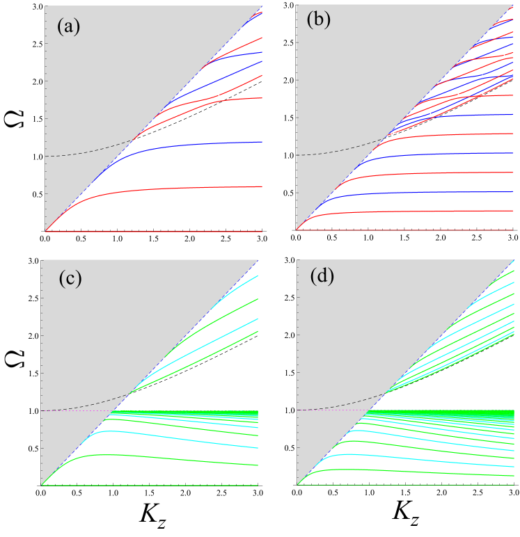
Figure 2: Band structure of symmetric and antisymmetric guided TM modes in nonlocal ((a,b), blue curves for symmetric, red curves for antisymmetric modes) and local ((c,d), cyan curves for symmetric, green curves for antisymmetric modes) WM slab models with $\varepsilon_{h}=3$, $\varepsilon_{d}=1$, for different slab thicknesses $\tilde{a}=(\omega_{h0}/c)a$: $\tilde{a}=3$ (a,c) and $\tilde{a}=7$ (b,d). The grey area corresponds to the leaky modes, $\Omega>K_{z}/\sqrt{\varepsilon_{d}}$. The dashed line $\Omega=\sqrt{1+K_{z}^{2}/\varepsilon_{h}}$ separates “fast” and “slow” guided modes, and the horizontal dotted line marks the lower boundary of the mode band gap $\Omega=1$ in the local WM slab model.

Moreover, an interesting band structure of guided modes appears in a nonlocal WM slab at frequencies

$$\sqrt{\omega_{h0}^{2}+\frac{c^{2}k_{z}^{2}}{\varepsilon_{h}}}<\omega<\frac{ck_{z}}{\sqrt{\varepsilon_{d}}}$$ (22)

(for $\varepsilon_{d}<\varepsilon_{h}$), corresponding to the “fast” guided modes, as seen in Fig. 2. Instead of series of almost parallel dispersion curves in the local WM slab model, in the nonlocal WM slab model the dispersion curves display the anticrossing behaviour. This effect is due to the coupling between different modes (the “fast” conventional waveguiding mode, and the “slow” surface mode) of the same parity, which is the effect conventionally observed in the coupled waveguide systems. The frequency splitting of the anti-crossing guided modes is proportional to the coupling strength, which in turn is proportional to the overlap integral of the two modes, which maximizes when the waveguide numbers of the two modes coincide. Near the anti-crossing points, the energy transfer between the coupled modes occurs, at the rate proportional to the coupling strength. Thus, it should be possible to excite both of the coupled modes by exciting only one mode of the pair with $K_{z}$ near their anti-crossing point. This can be particularly valuable for the excitation of the slow light modes by the free electromagnetic field (coupled to the fast waveguiding mode), which in its turn could be used in the optical information processing.

III.2 Spatial structure of guided TM modes

The spatial structure of the fields $E_{x}^{(\omega,k_{z})}(x)$, $E_{z}^{(\omega,k_{z})}(x)$, $B_{y}^{(\omega,k_{z})}(x)$ inside the slab is given by Eqs (27), with $E_{1}(n)$, $E_{3}(n)$ and $B_{2}(n)$ obtained from the linear system (30) as

$$E_{1}(n) = \frac{c^{2}}{\omega\varepsilon_{h}}\frac{k_{z}\alpha_{n}}{c^{2}k_{z}^{2}-\omega^{2}\varepsilon_{h}\varepsilon_{xx}(n)+c^{2}\alpha_{n}^{2}\varepsilon_{xx}(n)}\frac{2c^{2}}{a}\left[B_{y}^{(\omega,k_{z})}(0)-(-1)^{n}B_{y}^{(\omega,k_{z})}(a)\right],$$ (23)

$$E_{3}(n) = -i\frac{c^{2}}{\omega\varepsilon_{h}}\frac{c^{2}k_{z}^{2}-\omega^{2}\varepsilon_{h}\varepsilon_{xx}(n)}{c^{2}k_{z}^{2}-\omega^{2}\varepsilon_{h}\varepsilon_{xx}(n)+c^{2}\alpha_{n}^{2}\varepsilon_{xx}(n)}\frac{2}{a}\left[B_{y}^{(\omega,k_{z})}(0)-(-1)^{n}B_{y}^{(\omega,k_{z})}(a)\right],$$ (24)

$$B_{2}(n) = \frac{\alpha_{n}\varepsilon_{xx}(n)}{c^{2}k_{z}^{2}-\omega^{2}\varepsilon_{h}\varepsilon_{xx}(n)+c^{2}\alpha_{n}^{2}\varepsilon_{xx}(n)}\frac{2c^{2}}{a}\left[B_{y}^{(\omega,k_{z})}(0)-(-1)^{n}B_{y}^{(\omega,k_{z})}(a)\right],$$ (25)

in which the frequency $\omega$ is one of the solutions, for a given $k_{z}$, of the relevant dispersion equation from those obtained above, Eqs (17)–(19) and (18)–(20).

The spatial structure of the $E_{z}^{(\omega,k_{z})}(x)$ field of several consecutive symmetric modes in nonlocal WM slab is shown in Fig. 3.

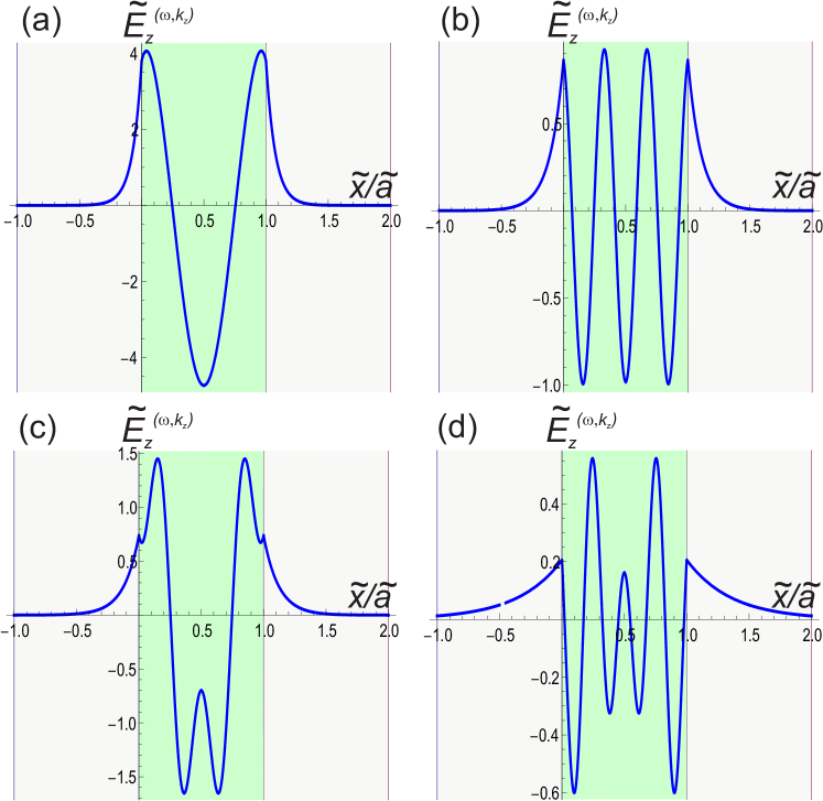
Figure 3: Spatial structure of $E_{z}^{(\omega,k_{z})}(x)$ of symmetric guided TM modes with $K_{z}=2.0$ in nonlocal WM slab model with $\varepsilon_{h}=3$, $\varepsilon_{d}=1$, for slab thickness $\tilde{a}=7$. The upper (a,b) and lower (c,d) rows show the spatial structure of the two consecutive “slow” modes (with $\Omega<\sqrt{1+K_{z}^{2}/\varepsilon_{h}}$) and the two consecutive “fast” modes (with $\Omega>\sqrt{1+K_{z}^{2}/\varepsilon_{h}}$), respectively (see Fig. 2 for their band structure at $K_{z}=2.0$).

III.3 Effect of losses in the host medium

Finally, we discuss the effect of losses present in the dielectric host media on the eigenmode dispersion. We introduce the losses by adding an imaginary part to the dielectric permittivity $\varepsilon_{h}$ of the host medium, and consider two different values of the imaginary part $\mathrm{Im}(\varepsilon_{h})=0.1,1.0$ (with $\mathrm{Re}(\varepsilon_{h})=3$), corresponding to weak and strong losses, respectively. The inclusion of the losses results in the emergence of negative imaginary part of the eigenfrequencies $\Gamma={\rm Im}(\Omega)<0$, which corresponds to the mode’s damping rate. The band structure of $|\Gamma|$ is shown in Fig. 4.

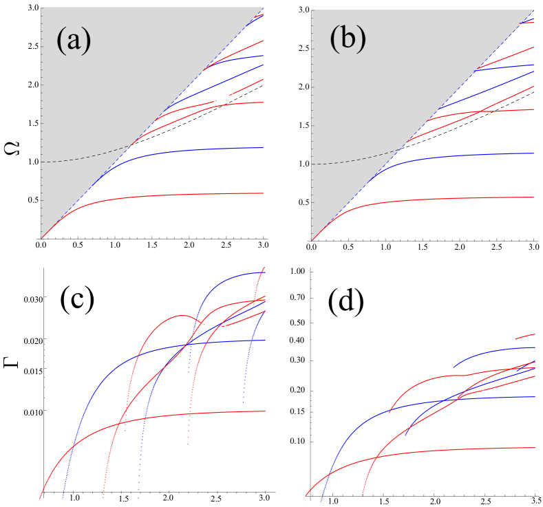
Figure 4: Band structure of the real (a,b) and negative imaginary (c,d) part of the eigenfrequencies for the case of low $\mathrm{Im}(\varepsilon_{h})=0.1$ (a,c) and high $\mathrm{Im}(\varepsilon_{h})=1.0$ (b,d) losses, for nonlocal WM slab with $\tilde{a}=3$, $\varepsilon_{d}=1$, ${\rm Re}(\varepsilon_{h})=3$.

We can see that damping decrements of the modes increase and then saturate at their respective resonances. Moreover, we notice the transition from the strong mode coupling regime resulting in the anticrossing behaviour for the real parts of mode frequencies, to the weak-coupling regime resulting in the anticrossing of the imaginary parts of the frequencies as the losses are increased. This effect is also widely observed in the microcavity physics, when the transition from the strong to the weak coupling regime manifests itself in the transition from the anticrossing of the modes frequencies to the anticrossing of the modes decay rates.

IV Conclusions

To conclude, we have studied the dispersion of the eigenmodes of the wire medium slab taking into account both the spatial dispersion and the losses in the structure. We have shown that the eigenmodes can be separated in two specific types: slow surface plasmon-polariton modes and fast conventional electromagnetic waveguide modes. We have also observed the strong pairwise coupling between slow and fast modes of the same parity resulting in the anticrossing of the dispersion curves. We stress that this effect arises only within the nonlocal approach, and thus has not been described previously. Moreover, we believe that the effect of the strong coupling between the slow and fast modes can be particularly valuable for the excitation of the slow light modes by the free electromagnetic field, which in its turn could be used in the optical information processing.

Appendix A Fourier method of solution for TM modes

Here we solve Eqs (4) for TM modes in the wire medium ($0\leq x\leq a$) using Fourier method. For this, we continue the fields and current densities, defined in the wire medium at $0\leq x\leq a$, to the region $-a\leq x<0$ as Kondratenko_Waveguides

$$E_{x}^{(\omega,k_{z})}(-x) = -E_{x}^{(\omega,k_{z})}(x)\ \text{(odd)}$$

$$j_{x}^{(\omega,k_{z})}(-x) = -j_{x}^{(\omega,k_{z})}(x)\ \text{(odd)}$$

$$E_{z}^{(\omega,k_{z})}(-x) = E_{z}^{(\omega,k_{z})}(x)\ \text{(even)}$$ (26)

$$j_{z}^{(\omega,k_{z})}(-x) = j_{z}^{(\omega,k_{z})}(x)\ \text{(even)}$$

$$B_{y}^{(\omega,k_{z})}(-x) = -B_{y}^{(\omega,k_{z})}(x)\ \text{(odd)}$$

and then continue these fields and current densities, now defined at $-a\leq x\leq a$, periodically to the entire $x$ axis, with a period of $2a$: $E_{x}^{(\omega,k_{z})}(x+2a)=E_{x}^{(\omega,k_{z})}(x)$, etc. Thus continued fields and current densities are defined for all $x$, and coincide with the physical fields and current densities inside the wire medium slab. This mathematical trick allows us to solve Eqs (4) for fields inside the WM slab by seeking the solutions of Eqs (4), for thus continued fields and current densities, in the form of Fourier series

$$E_{x}^{(\omega,k_{z})}(x) = \sum_{n=0}^{\infty}{E_{1}(n)\sin(\alpha_{n}x)},$$

$$j_{x}^{(\omega,k_{z})}(x) = \sum_{n=0}^{\infty}{j_{1}(n)\sin(\alpha_{n}x)},$$

$$E_{z}^{(\omega,k_{z})}(x) = \left.\sum_{n=0}^{\infty}\right.^{\prime}{E_{3}(n)\cos(\alpha_{n}x)},$$ (27)

$$j_{z}^{(\omega,k_{z})}(x) = \left.\sum_{n=0}^{\infty}\right.^{\prime}{j_{3}(n)\cos(\alpha_{n}x)},$$

$$B_{y}^{(\omega,k_{z})}(x) = \sum_{n=0}^{\infty}{B_{2}(n)\sin(\alpha_{n}x)},$$

where $\alpha_{n}=n\pi/a$, and $\sum^{\prime}$ implies that the $n=0$ term of the sum should be multiplied by $1/2$. Note that in writing the above Fourier series, the symmetries of the continued fields and current densities, introduced by Eqs (26), have been taken into account. (Note that, in order to find the physical fields outside the slab, one needs to solve a separate problem for fields at $x<0$ and $x>a$, with $j_{x}=j_{z}=0$, and then match the solutions for the obtained fields inside and outside the slab, using continuity of tangential components of $\mathbf{E,B}$ at the slab boundaries $x=0,\ a$. This yields the dispersion equation for the modes of such system; see Sec II.3.)

Under the condition of zero normal component of the effective WM current density at the WM slab boundaries, $j_{x}(x=0)=j_{x}(x=a)=0$, the constitutive relations for the WM slab are the same as those for the unbounded WM, and the Fourier coefficients of the current densities $j_{x}$ and $j_{z}$ are obtained as Kondratenko_Waveguides

$$j_{i}(n)=\sum_{k=1}^{3}\sigma_{ik}(n)E_{k}(n),$$ (28)

where $\sigma_{ik}(n)$ is the conductivity tensor of the bulk WM, in which $k_{x}=\alpha_{n}$:

$$\sigma_{ik}(n)=i\omega\varepsilon_{0}\left[\delta_{ik}-\varepsilon_{ik}(n)\right],$$ (29)

where $\varepsilon_{ik}(n)$ is given by (1) with $k_{x}=\alpha_{n}=n\pi/a$.

From Eqs (4), using (28) and (29), we obtain, taking into account that the $B_{y}^{(\omega,k_{z})}(x)$ field is discontinuous at the boundaries $x=0,a$:

$$ik_{z}E_{1}(n)+\alpha_{n}E_{3}(n)-i\omega B_{2}(n) = 0,$$

$$-i\omega\varepsilon_{h}\varepsilon_{xx}(n)E_{1}(n)+c^{2}ik_{z}B_{2}(n) = 0,$$

$$i\omega\varepsilon_{h}E_{3}(n)+c^{2}\alpha_{n}B_{2}(n) = \frac{2c^{2}}{a}\left[B_{y}^{(\omega,k_{z})}(0)-(-1)^{n}B_{y}^{(\omega,k_{z})}(a)\right].$$ (30)

From this linear system, we obtain $E_{3}(n)$ as

$$E_{3}(n)=-i\frac{c^{2}}{\omega\varepsilon_{h}}\frac{c^{2}k_{z}^{2}-\omega^{2}\varepsilon_{h}\varepsilon_{xx}(n)}{c^{2}k_{z}^{2}-\omega^{2}\varepsilon_{h}\varepsilon_{xx}(n)+c^{2}\alpha_{n}^{2}\varepsilon_{xx}(n)}\frac{2}{a}\left[B_{y}^{(\omega,k_{z})}(0)-(-1)^{n}B_{y}^{(\omega,k_{z})}(a)\right].$$ (31)

Finally, substituting $E_{3}(n)$ into $E_{z}^{(\omega,k_{z})}(x)=\sum^{\prime}{E_{3}(n)\cos(\alpha_{n}x)}$, and taking $x=0,a$, we obtain the impedance relations between the tangential components of electric and magnetic fields at the WM slab boundaries, shown in Eqs (5)–(6).

Appendix B Alternative method

In this section we present an alternative way to obtain the dispersion of the eigenmodes in the wire medium slab based on the additional boundary conditions technique MGS . Within the local homogenization model for the case of perfectly conducting wires the principal components of the dielectric permittivity tensor become $[\infty,\varepsilon_{h},\varepsilon_{h}]$. In this case only a TEM polarized mode (a kind of modes that is useful for transmission line mode’s polarization, electric and magnetic components of such type of modes are perpendicular to the direction of propagation) can be excited in the wire media slab. The eigenmode dispersion equation can then be recovered by applying conventional continuity boundary conditions for electric and magnetic fields at both interfaces of the slab. However, the situation becomes more complicated if we account for nonlocality Maslovski_PRB_2009 , i.e. spatial dispersion of the dielectric permittivity. In this case, wire media slab supports propagation of both TEM and TM polarized waves. It is evident then that we need an additional boundary condition in order to obtain the eigenmode dispersion equation. The additional boundary condition states that the current at the ends of the wires is exactly zero and can be rewritten in the following form:

$$\left[\frac{\partial^{2}H_{z}}{\partial x^{2}}+\varepsilon_{h}\left(\frac{\omega}{c}\right)^{2}H_{z}\right]_{x=0,a}=0,$$ (32)

where square brackets denote the difference at the corresponding interface: e.g., $[f(x)]_{x=0}=f(x=0^{+})-f(x=0^{-})$. Now when we have the three boundary conditions (continuity of tangential components of electric and magnetic fields, and Eq. (32)) at each interface ($x=0,a$), we write down the fields inside the wire medium slab. We would like to obtain both the eigenmode dispersion equation and the transmission and reflection coefficients for the wire medium slab and thus we consider the case when the electromagnetic field $(\mathbf{E}_{\rm inc},\mathbf{H}_{\rm inc})$ is incident on the wire medium slab. The electromagnetic fields in the three regions can be written in the form AE ; AE2 :

$$\frac{H(x)}{H_{\rm inc}}=\left\{\begin{array}[]{lcl}e^{ik_{x}x}+Re^{-ik_{x}x},\quad x<0\\[5.69054pt] \begin{array}[]{lcl}A_{-}^{\rm TM}e^{-\frac{k_{p}\kappa_{x}}{\sqrt{\varepsilon_{h}}}(x-a/2)}\\ +A_{+}^{\rm TM}e^{+\frac{k_{p}\kappa_{x}}{\sqrt{\varepsilon_{h}}}(x-a/2)}\\ +A_{-}^{\rm TEM}e^{ik_{p}\Omega(x-a/2)}\\ +A_{+}^{\rm TEM}e^{-ik_{p}\Omega(x-a/2)},\\ \end{array}\quad 0\leq x\leq a\\[25.60747pt] Te^{ik_{x}(x-a)},\quad x>a,\vphantom{\frac{A}{A}}\\ \end{array}\right.$$ (33)

where $R$ and $T$ are unknown reflection and transmission coefficients. $A_{\pm}^{\rm TM}$ and $A_{\pm}^{\rm TEM}$ are unknown amplitudes of TM and TEM waves that correspond to forward and backward propagating waves along the $x$ axis from Fig. 1. We normalized this system to the magnetic field of the incident wave $H_{\rm inc}$. If we then apply three boundary conditions at each interface we get the linear system for the amplitudes of the fields:

$$\left(\begin{array}[]{cccccc}-1&e^{\frac{k_{p}\kappa_{x}}{\sqrt{\varepsilon_{h}}}a/2}&e^{-\frac{k_{p}\kappa_{x}}{\sqrt{\varepsilon_{h}}}a/2}&e^{-ik_{p}a\Omega/2}&e^{ik_{p}a\Omega/2}&0\\ ik_{x}&-\frac{k_{p}\kappa_{x}}{\varepsilon_{h}^{3/2}}e^{\frac{k_{p}\kappa_{x}}{\sqrt{\varepsilon_{h}}}a/2}&\frac{k_{p}\kappa_{x}}{\varepsilon_{h}^{3/2}}e^{-\frac{k_{p}\kappa_{x}}{\sqrt{\varepsilon_{h}}}a/2}&\frac{ik_{p}\Omega}{\varepsilon_{h}}e^{-ik_{p}a\Omega/2}&-\frac{ik_{p}\Omega}{\varepsilon_{h}}e^{ik_{p}a\Omega/2}&0\\ k_{x}^{2}-\left(\frac{\omega}{c}\right)^{2}&qe^{\frac{k_{p}\kappa_{x}}{\sqrt{\varepsilon_{h}}}a/2}&qe^{-\frac{k_{p}\kappa_{x}}{\sqrt{\varepsilon_{h}}}a/2}&0&0&0\\ 0&e^{-\frac{k_{p}\kappa_{x}}{\sqrt{\varepsilon_{h}}}a/2}&e^{\frac{k_{p}\kappa_{x}}{\sqrt{\varepsilon_{h}}}a/2}&e^{ik_{p}a\Omega/2}&e^{-ik_{p}a\Omega/2}&-1\\ 0&-\frac{k_{p}\kappa_{x}}{\varepsilon_{h}^{3/2}}e^{-\frac{k_{p}\kappa_{x}}{\sqrt{\varepsilon_{h}}}a/2}&\frac{k_{p}\kappa_{x}}{\varepsilon_{h}^{3/2}}e^{\frac{k_{p}\kappa_{x}}{\sqrt{\varepsilon_{h}}}a/2}&\frac{ik_{p}\Omega}{\varepsilon_{h}}e^{ik_{p}a\Omega/2}&-\frac{ik_{p}\Omega}{\varepsilon_{h}}e^{-ik_{p}a\Omega/2}&-ik_{x}\\ 0&qe^{-\frac{k_{p}\kappa_{x}}{\sqrt{\varepsilon_{h}}}a/2}&qe^{\frac{k_{p}\kappa_{x}}{\sqrt{\varepsilon_{h}}}a/2}&0&0&k_{x}^{2}-\left(\frac{\omega}{c}\right)^{2}\\ \end{array}\right)$$ (40)

$$\times\left(\begin{array}[]{c}R\\ A_{-}^{\rm TM}\\ A_{+}^{\rm TM}\\ A_{-}^{\rm TEM}\\ A_{+}^{\rm TEM}\\ T\\ \end{array}\right)=\left(\begin{array}[]{c}1\\ ik_{x}\\ -k_{x}^{2}+\left(\frac{\omega}{c}\right)^{2}\\ 0\\ 0\\ 0\\ \end{array}\right),\qquad$$ (53)

where $q=\left(k_{p}\kappa_{x}/\sqrt{\varepsilon_{h}}\right)^{2}+\varepsilon_{h}\left(\omega/c\right)^{2}$. Solving the system and changing to dimensionless variables introduced above in Sec II.2, we get the transmission and reflection coefficients as well as amplitudes of all the modes in the structure:

$$T=\left[1+\frac{1}{\varepsilon_{h}\left(K_{z}^{2}+\varepsilon_{h}\right)\sqrt{K_{z}^{2}-\Omega^{2}}}\left(-\varepsilon_{h}^{3/2}\Omega\tan\left(\varepsilon_{h}^{1/2}\Omega\tilde{a}/2\right)+K_{z}^{2}\kappa_{x}\tanh\left(\kappa_{x}\tilde{a}/2\right)\right)\right]^{-1}$$

$$-\left[1+\frac{1}{\varepsilon_{h}\left(K_{z}^{2}+\varepsilon_{h}\right)\sqrt{K_{z}^{2}-\Omega^{2}}}\left(\varepsilon_{h}^{3/2}\Omega\cot\left(\varepsilon_{h}^{1/2}\Omega\tilde{a}/2\right)+K_{z}^{2}\kappa_{x}\coth\left(\kappa_{x}\tilde{a}/2\right)\right)\right]^{-1},$$

(54)

$$R=\left[1+\frac{1}{\varepsilon_{h}\left(K_{z}^{2}+\varepsilon_{h}\right)\sqrt{K_{z}^{2}-\Omega^{2}}}\left(-\varepsilon_{h}^{3/2}\Omega\tan\left(\varepsilon_{h}^{1/2}\Omega\tilde{a}/2\right)+K_{z}^{2}\kappa_{x}\tanh\left(\kappa_{x}\tilde{a}/2\right)\right)\right]^{-1}$$

$$+\left[1+\frac{1}{\varepsilon_{h}\left(K_{z}^{2}+\varepsilon_{h}\right)\sqrt{K_{z}^{2}-\Omega^{2}}}\left(\varepsilon_{h}^{3/2}\Omega\cot\left(\varepsilon_{h}^{1/2}\Omega\tilde{a}/2\right)+K_{z}^{2}\kappa_{x}\coth\left(\kappa_{x}\tilde{a}/2\right)\right)\right]^{-1}-1,$$

(55)

$$A_{-}^{TM}=\frac{1}{2\left(1+\frac{\varepsilon_{h}}{K_{z}^{2}}\right)}\left(\frac{\mbox{sech}\left(\kappa_{x}\tilde{a}/2\right)}{1+\frac{1}{\varepsilon_{h}\left(K_{z}^{2}+\varepsilon_{h}\right)\sqrt{K_{z}^{2}-\Omega^{2}}}\left(-\varepsilon_{h}^{3/2}\Omega\tan\left(\varepsilon_{h}^{1/2}\Omega\tilde{a}/2\right)+K_{z}^{2}\kappa_{x}\tanh\left(\kappa_{x}\tilde{a}/2\right)\right)}\right.$$

$$\left.+\frac{\mbox{csch}\left(\kappa_{x}\tilde{a}/2\right)}{1+\frac{1}{\varepsilon_{h}\left(K_{z}^{2}+\varepsilon_{h}\right)\sqrt{K_{z}^{2}-\Omega^{2}}}\left(\varepsilon_{h}^{3/2}\Omega\cot\left(\varepsilon_{h}^{1/2}\Omega\tilde{a}/2\right)+K_{z}^{2}\kappa_{x}\coth\left(\kappa_{x}\tilde{a}/2\right)\right)}\right),$$

(56)

$$A_{+}^{TM}=\frac{1}{2\left(1+\frac{\varepsilon_{h}}{K_{z}^{2}}\right)}\left(\frac{\mbox{sech}\left(\kappa_{x}\tilde{a}/2\right)}{1+\frac{1}{\varepsilon_{h}\left(K_{z}^{2}+\varepsilon_{h}\right)\sqrt{K_{z}^{2}-\Omega^{2}}}\left(-\varepsilon_{h}^{3/2}\Omega\tan\left(\varepsilon_{h}^{1/2}\Omega\tilde{a}/2\right)+K_{z}^{2}\kappa_{x}\tanh\left(\kappa_{x}\tilde{a}/2\right)\right)}\right.$$

$$\left.-\frac{\mbox{csch}\left(\kappa_{x}\tilde{a}/2\right)}{1+\frac{1}{\varepsilon_{h}\left(K_{z}^{2}+\varepsilon_{h}\right)\sqrt{K_{z}^{2}-\Omega^{2}}}\left(\varepsilon_{h}^{3/2}\Omega\cot\left(\varepsilon_{h}^{1/2}\Omega\tilde{a}/2\right)+K_{z}^{2}\kappa_{x}\coth\left(\kappa_{x}\tilde{a}/2\right)\right)}\right),$$

(57)

$$A_{-}^{TEM}=\frac{1}{2\left(1+\frac{K_{z}^{2}}{\varepsilon_{h}}\right)}\left(\frac{\mbox{sec}\left(\varepsilon_{h}^{1/2}\Omega\tilde{a}/2\right)}{1+\frac{1}{\varepsilon_{h}\left(K_{z}^{2}+\varepsilon_{h}\right)\sqrt{K_{z}^{2}-\Omega^{2}}}\left(-\varepsilon_{h}^{3/2}\Omega\tan\left(\varepsilon_{h}^{1/2}\Omega\tilde{a}/2\right)+K_{z}^{2}\kappa_{x}\tanh\left(\kappa_{x}\tilde{a}/2\right)\right)}\right.$$

$$\left.+\frac{i\mbox{cosec}\left(\varepsilon_{h}^{1/2}\Omega\tilde{a}/2\right)}{1+\frac{1}{\varepsilon_{h}\left(K_{z}^{2}+\varepsilon_{h}\right)\sqrt{K_{z}^{2}-\Omega^{2}}}\left(\varepsilon_{h}^{3/2}\Omega\cot\left(\varepsilon_{h}^{1/2}\Omega\tilde{a}/2\right)+K_{z}^{2}\kappa_{x}\coth\left(\kappa_{x}\tilde{a}/2\right)\right)}\right),$$

(58)

$$A_{+}^{TEM}=\frac{1}{2\left(1+\frac{K_{z}^{2}}{\varepsilon_{h}}\right)}\left(\frac{\mbox{sec}\left(\varepsilon_{h}^{1/2}\Omega\tilde{a}/2\right)}{1+\frac{1}{\varepsilon_{h}\left(K_{z}^{2}+\varepsilon_{h}\right)\sqrt{K_{z}^{2}-\Omega^{2}}}\left(-\varepsilon_{h}^{3/2}\Omega\tan\left(\varepsilon_{h}^{1/2}\Omega\tilde{a}/2\right)+K_{z}^{2}\kappa_{x}\tanh\left(\kappa_{x}\tilde{a}/2\right)\right)}\right.$$

$$\left.-\frac{i\mbox{cosec}\left(\varepsilon_{h}^{1/2}\Omega\tilde{a}/2\right)}{1+\frac{1}{\varepsilon_{h}\left(K_{z}^{2}+\varepsilon_{h}\right)\sqrt{K_{z}^{2}-\Omega^{2}}}\left(\varepsilon_{h}^{3/2}\Omega\cot\left(\varepsilon_{h}^{1/2}\Omega\tilde{a}/2\right)+K_{z}^{2}\kappa_{x}\coth\left(\kappa_{x}\tilde{a}/2\right)\right)}\right),$$

(59)

So we get dispersion relations explicitly from the denominator of expressions (54)–(59):

$$1+\frac{1}{\varepsilon_{h}\left(K_{z}^{2}+\varepsilon_{h}\right)\sqrt{K_{z}^{2}-\Omega^{2}}}\left(-\varepsilon_{h}^{3/2}\Omega\tan\left(\varepsilon_{h}^{1/2}\Omega\tilde{a}/2\right)+K_{z}^{2}\kappa_{x}\tanh\left(\kappa_{x}\tilde{a}/2\right)\right)=0,$$ (60)

$$1+\frac{1}{\varepsilon_{h}\left(K_{z}^{2}+\varepsilon_{h}\right)\sqrt{K_{z}^{2}-\Omega^{2}}}\left(\varepsilon_{h}^{3/2}\Omega\cot\left(\varepsilon_{h}^{1/2}\Omega\tilde{a}/2\right)+K_{z}^{2}\kappa_{x}\coth\left(\kappa_{x}\tilde{a}/2\right)\right)=0.$$ (61)

These formulae fully coincide with (17,18). This fact confirms the results of both methods.

References

• (1) C.R. Simovsky, P.A. Belov, A.V. Atrashenko, and Yu. S. Kivshar, Adv. Mat. 24, 4229 (2012).
• (2) M.G. Silveirinha, P.A. Belov, and C.R. Simovski, Phys. Rev. B 75, 035108 (2007).
• (3) P.A. Belov, Y. Zhao, S. Tse, P. Ikonen, M.G. Silveirinha, C.R. Simovski, S.A. Tretyakov, Y. Hao, and C. Parini, Phys.Rev. B 77, 193108 (2008).
• (4) P.A. Belov, G.K. Palikaras, Y.Zhao, A.Rahman, C.R. Simovski, Y.Hao, and C. Parini, Appl. Phys. Lett. 97, 191905 (2010).
• (5) J. Yao, Zh. Liu, Yo. Liu, Yu. Wang, C. Sun, G. Bartal, A. M. Stacy, and X. Zhang, Science, 321, 930 (2008).
• (6) P. Ginzburg, F. Rodríguez Fortuño, G.A. Wurtz, W. Dickson, A. Murphy, F. Morgan, R.J. Pollard, I. Iorsh, A. Atrashchenko, P.A. Belov, Yu.S. Kivshar, A. Nevet, G. Ankonina, M. Orenstein, A.V. Zayats, Optics Express, 21, 14907 (2013).
• (7) P.A. Belov and M.G. Silveirinha, Phys. Rev. E 73, 056607 (2006).
• (8) Y. Zhao, G. Palikaras, P.A. Belov, R.F Dubrovka, C.R. Simovski, Y. Hao, and C.G. Parini, New J. Phys. 12, 103045 (2010).
• (9) S.A. Maier, S.R. Andrews, L. Martin-Moreno, and F. J. Garcia-Vidal, Phys. Rev. Lett. 97, 176805 (2006).
• (10) M. Navarro-Cia, M. Beruete, S. Agrafiotis, F. Falcone, M. Sorolla, and S.A. Maier, Opt. Exp. 17, 18184 (2009).
• (11) E.K. Stone and E. Hendry, Phys. Rev. B 84, 035418 (2011).
• (12) F. Lemoult, G. Lerosey, J. Rosny, and M. Fink, Phys. Rev. Lett. 104, 203901 (2010).
• (13) F. Lemoult, M. Fink, and G. Lerosey, Nature Commun. 3, 889 (2012).
• (14) F. Lemoult, N. Kaina, M. Fink, and G. Lerosey, Nature Phys. 9, 55 (2013).
• (15) F. Lemoult, M. Fink, and G. Lerosey, Waves in Random and Complex Media 21, 591 (2011).
• (16) P.A. Belov, R. Marques, S.I. Maslovski, I.S. Nefedov, M. Silveirinha, C.R. Simovski, S.A. Tretyakov, Phys. Rev. B, 67, 113103 (2003)
• (17) S.I. Maslovski, M.G. Silveirinha, Phys.Rev. B, 80, 245101 (2009).
• (18) A.N. Kondratenko, Plasma Waveguides, Atomizdat (1976).
• (19) A.E. Ageyskiy, S.Y. Kosulnikov, P.A. Belov, Opt. Spectrosc. 110, 572 (2011).
• (20) A.E. Ageyskiy, S.Y. Kosulnikov, S.I. Maslovski, Y.S. Kivshar, P.A. Belov, Phys. Rev. B 85, 033105 (2012).
• (21) O. Luukkonen, C. R. Simovski, A. V. Raisanen, S. A. Tretyakov, IEEE Trans. Microw. Theory Tech. 56, 1624 (2008).
• (22) A. F. Alexandrov, L. S. Bogdankevich, A. A. Rukhadze, Principles of Plasma Electrodynamics, Springer-Verlag, (1984).
• (23) M. Silveirinha, IEEE Trans. on Antennas and Propagation 54, 1766 (2006).