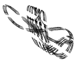
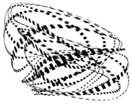
Lagrangian tori near resonances of near-integrable Hamiltonian systems

Medvedev A. G.111Lomonosov Moscow State University, Neishtadt A. I.222Space Research Institute of RAS, Department of Mathematical Sciences, Loughborough University, Treschev D. V.333Steklov Mathematical Institute of RAS
Abstract

In this paper we study families of Lagrangian tori that appear in a neighborhood of a resonance of a near-integrable Hamiltonian system. Such families disappear in the ‘‘integrable’’ limit ε0𝜀0\varepsilon\to 0. Dynamics on these tori is oscillatory in the direction of the resonance phases and rotating with respect to the other (non-resonant) phases.

We also show that, if multiplicity of the resonance equals one, generically these tori occupy a set of large relative measure in the resonant domains in the sense that the relative measure of the remaining ‘‘chaotic’’ set is of order ε𝜀\sqrt{\varepsilon}. Therefore for small ε>0𝜀0\varepsilon>0 a random initial condition in a ε𝜀\sqrt{\varepsilon}-neighborhood of a single resonance occurs inside this set (and therefore generates a quasi-periodic motion) with a probability much larger than in the ‘‘chaotic’’ set.

We present results of numerical simulations and discuss the form of projection of such tori to the action space.

1 Projection of trajectories to the action space

Consider a symplectic map

(y,x)(y+,x+),y2,x𝕋2formulae-sequencemaps-to𝑦𝑥subscript𝑦subscript𝑥formulae-sequence𝑦superscript2𝑥superscript𝕋2\displaystyle(y,x)\mapsto(y_{+},x_{+}),\qquad y\in\mathbb{R}^{2},\quad x\in\mathbb{T}^{2} (1.1)
y+=yεV/x,x+=x+y+,V=V(x).formulae-sequencesubscript𝑦𝑦𝜀𝑉𝑥formulae-sequencesubscript𝑥𝑥subscript𝑦𝑉𝑉𝑥\displaystyle y_{+}=y-\varepsilon\,\partial V/\partial x,\quad x_{+}=x+y_{+},\qquad V=V(x). (1.2)

For ε=0𝜀0\varepsilon=0 the dynamics is integrable and (y,x)𝑦𝑥(y,x) are action-angle variables on the phase space 2×𝕋2superscript2superscript𝕋2\mathbb{R}^{2}\times\mathbb{T}^{2}. We choose for definiteness

V=a1cos(x1+φ1)+a2cos(x2+φ2)+a3cos(x1x2+φ3)𝑉subscript𝑎1subscript𝑥1subscript𝜑1subscript𝑎2subscript𝑥2subscript𝜑2subscript𝑎3subscript𝑥1subscript𝑥2subscript𝜑3V=a_{1}\cos(x_{1}+\varphi_{1})+a_{2}\cos(x_{2}+\varphi_{2})+a_{3}\cos(x_{1}-x_{2}+\varphi_{3})

with constant a1,a2,a3,φ1,φ2,φ3subscript𝑎1subscript𝑎2subscript𝑎3subscript𝜑1subscript𝜑2subscript𝜑3a_{1},a_{2},a_{3},\varphi_{1},\varphi_{2},\varphi_{3}. We study trajectories numerically having in mind the idea to observe some interesting images and then find theoretic explanations. To visualize objects (closures of trajectories) lying in the 4-dimensional phase space, we project them to the action plane 2={y}superscript2𝑦\mathbb{R}^{2}=\{y\}. We fix aj1similar-tosubscript𝑎𝑗1a_{j}\sim 1, φjsubscript𝜑𝑗\varphi_{j}, ε1/10similar-to𝜀110\varepsilon\sim 1/10, take a random initial condition and see.

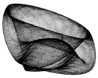
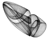
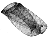
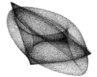
Typical images are presented on Fig. 1. They can be easily identified with ordinary KAM-tori. We see typical singularities (folds and pleats) of Lagrangian projections (these singularities are presented for example, in [2]).

Refer to caption
Refer to caption
Refer to caption
Figure 1: KAM-tori

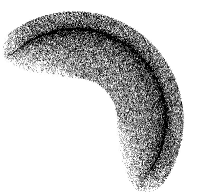
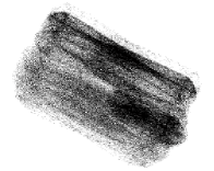
It is also easy to observe chaotic trajectories, Fig. 2. The trajectories presented in Fig. 2, right and center, are situated near KAM-tori, but chaotic effects create a small ‘‘defocusing’’ in comparison with tori from Fig. 1.
Refer to caption
Refer to caption
Refer to caption
Figure 2: Chaotic trajectories: near KAM-tori (center,right) and near a strong resonance (left)

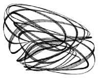
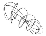
Trying more initial conditions, it is possible to obtain more mysterious objects, Fig. 3, which look like closed ribbons. Further attempts lead to more exotic images, Fig. 4, looking as finite sequences of spots.
Refer to caption
Refer to caption
Refer to caption
Figure 3: Closed "ribbons"
Refer to caption
Refer to caption
Figure 4: Another type of quasi-periodic trajectories, ‘‘sequences of spots’’

In this paper we discuss a mechanism which generates such structures. In particular we show that these objects form sets of positive measure in the phase space. Hence probability to observe them is also positive.

2 Lower-dimensional tori near resonances

As usual it is more convenient to write formulas for flows although numerics are faster, simpler and more precise for maps. Consider a real-analytic near-integrable Hamiltonian system

X˙=H/Y,Y˙=H/X,Y𝒟N,X𝕋N.formulae-sequenceformulae-sequence˙𝑋𝐻𝑌formulae-sequence˙𝑌𝐻𝑋𝑌𝒟superscript𝑁𝑋superscript𝕋𝑁\displaystyle\dot{X}=\partial H/\partial Y,\quad\dot{Y}=-\partial H/\partial X,\qquad Y\in{\cal D}\subset\mathbb{R}^{N},\quad X\in\mathbb{T}^{N}. (2.1)
H=H0(Y)+εH1(Y,X)+O(ε2),ε0.formulae-sequence𝐻subscript𝐻0𝑌𝜀subscript𝐻1𝑌𝑋𝑂superscript𝜀2𝜀0\displaystyle H=H_{0}(Y)+\varepsilon H_{1}(Y,X)+O(\varepsilon^{2}),\qquad\varepsilon\geq 0. (2.2)

Below we use the following notation for such a system:

(P,ωP,H),P=𝒟×𝕋N,ωP=dYdX,formulae-sequence𝑃subscript𝜔𝑃𝐻𝑃𝒟superscript𝕋𝑁subscript𝜔𝑃𝑑𝑌𝑑𝑋(P,\omega_{P},H),\qquad P={\cal D}\times\mathbb{T}^{N},\quad\omega_{P}=dY\wedge dX,

where the symplectic manifold (P,ωP)𝑃subscript𝜔𝑃(P,\omega_{P}) is the phase space.

The map (1.1)–(1.2) can be regarded as the Poincaré map for some system (2.1)–(2.2) with N=3𝑁3N=3 on an energy level Mh={H=h=const}subscript𝑀𝐻constM_{h}=\{H=h=\mbox{const}\} (see for example [11]). Hence the dimension of the phase space 6=2N62𝑁6=2N drops by 1 because of the reduction to Mhsubscript𝑀M_{h} and by another 1 because of the passage to a (hyper)surface ΣMhΣsubscript𝑀\Sigma\subset M_{h} transversal to the flow. Below N3𝑁3N\geq 3 is arbitrary.

The vector ν(Y)=H0/Y𝜈𝑌subscript𝐻0𝑌\nu(Y)=\partial H_{0}/\partial Y is called an unperturbed frequency. For a fixed Y=Y0𝑌superscript𝑌0Y=Y^{0} we have a fixed frequency ν0=ν(Y0)superscript𝜈0𝜈superscript𝑌0\nu^{0}=\nu(Y^{0}). Any equation

ν0,K=0,KN{0}formulae-sequencesuperscript𝜈0𝐾0𝐾superscript𝑁0\langle\nu^{0},K\rangle=0,\qquad K\in\mathbb{Z}^{N}\setminus\{0\} (2.3)

is called a resonance. The word ‘‘resonance’’ is also attributed to the integer vector K𝐾K, satisfying (2.3).

Given a constant ν0Nsuperscript𝜈0superscript𝑁\nu^{0}\in\mathbb{R}^{N} all the corresponding resonances K𝐾K (together with 0N0superscript𝑁0\in\mathbb{Z}^{N}) form a resonance \mathbb{Z}-module

g(ν0)={KN:K is a resonance}{0}.𝑔superscript𝜈0conditional-set𝐾superscript𝑁𝐾 is a resonance0g(\nu^{0})=\{K\in\mathbb{Z}^{N}:K\mbox{ is a resonance}\}\cup\{0\}.

If g(ν0)=0𝑔superscript𝜈00g(\nu^{0})=0, the frequency vector ν0superscript𝜈0\nu^{0} is said to be nonresonant. We define

l=l(ν0)=rank(g(ν0)),m=m(ν0)=Nl,formulae-sequence𝑙𝑙superscript𝜈0rank𝑔superscript𝜈0𝑚𝑚superscript𝜈0𝑁𝑙l=l(\nu^{0})=\operatorname{rank}(g(\nu^{0})),\quad m=m(\nu^{0})=N-l,

where rank(g(ν0))rank𝑔superscript𝜈0\operatorname{rank}(g(\nu^{0})) is the number of generators in g(ν0)𝑔superscript𝜈0g(\nu^{0}). Informally speaking, l𝑙l is the number of independent resonances for the frequency vector ν0superscript𝜈0\nu^{0}. Invariant torus is called resonant (nonresonant) if the dynamics on the torus is quasi-periodic with a resonant (nonresonant) frequency vector. Any torus

𝕋Y0N={(Y,X):Y=Y0}subscriptsuperscript𝕋𝑁superscript𝑌0conditional-set𝑌𝑋𝑌superscript𝑌0\mathbb{T}^{N}_{Y^{0}}=\{(Y,X):Y=Y^{0}\}

is invariant with respect to the unperturbed flow

(Y,X)(Y,X+ν(Y)t),t.formulae-sequencemaps-to𝑌𝑋𝑌𝑋𝜈𝑌𝑡𝑡(Y,X)\mapsto(Y,X+\nu(Y)t),\qquad t\in\mathbb{R}.

Then 𝕋Y0Nsubscriptsuperscript𝕋𝑁superscript𝑌0\mathbb{T}^{N}_{Y^{0}} is foliated by the m𝑚m-tori

𝕋Y0,X0m=closure({(Y,X):Y=Y0,X=X0+ν0t,t}).subscriptsuperscript𝕋𝑚superscript𝑌0superscript𝑋0closureconditional-set𝑌𝑋formulae-sequence𝑌superscript𝑌0formulae-sequence𝑋superscript𝑋0superscript𝜈0𝑡𝑡\mathbb{T}^{m}_{Y^{0},X^{0}}=\mbox{closure}\big{(}\big{\{}(Y,X):Y=Y^{0},\;X=X^{0}+\nu^{0}t,\;t\in\mathbb{R}\big{\}}\big{)}.

Computing frequency vector corresponding to the unperturbed quasi-periodic motion on 𝕋Y0,X0msubscriptsuperscript𝕋𝑚superscript𝑌0superscript𝑋0\mathbb{T}^{m}_{Y^{0},X^{0}}, it is easy to show that the tori 𝕋Y0,X0msubscriptsuperscript𝕋𝑚superscript𝑌0superscript𝑋0\mathbb{T}^{m}_{Y^{0},X^{0}} are non-resonant.

Note that in the non-resonant case (l=0)𝑙0(l=0) we have 𝕋Y0,X0m=𝕋Y0msubscriptsuperscript𝕋𝑚superscript𝑌0superscript𝑋0subscriptsuperscript𝕋𝑚superscript𝑌0\mathbb{T}^{m}_{Y^{0},X^{0}}=\mathbb{T}^{m}_{Y^{0}} for any X0𝕋Nsuperscript𝑋0superscript𝕋𝑁X^{0}\in\mathbb{T}^{N}. If l>0𝑙0l>0 then mN𝑚𝑁m\neq N and the foliation is non-trivial.

If l>0𝑙0l>0 then a generic perturbation destroys 𝕋Y0msubscriptsuperscript𝕋𝑚superscript𝑌0\mathbb{T}^{m}_{Y^{0}}, [9]. However generically some tori 𝕋Y0,X0msubscriptsuperscript𝕋𝑚superscript𝑌0superscript𝑋0\mathbb{T}^{m}_{Y^{0},X^{0}} survive a perturbation even if ν0superscript𝜈0\nu^{0} is resonant. To present the corresponding result, we fix a \mathbb{Z}-module gn𝑔superscript𝑛g\subset\mathbb{Z}^{n}. Consider the resonance set

Σg={Y𝒟:g(ν(Y))=g}.subscriptΣ𝑔conditional-set𝑌𝒟𝑔𝜈𝑌𝑔\Sigma_{g}=\{Y\in{\cal D}:g(\nu(Y))=g\}.

Under natural non-degeneracy conditions444the functions K(j),/YH0(Y)superscript𝐾𝑗𝑌subscript𝐻0𝑌\langle K^{(j)},\partial/\partial Y\rangle H_{0}(Y) are independent in 𝒟𝒟{\cal D} where K(1),,K(l)superscript𝐾1superscript𝐾𝑙K^{(1)},\ldots,K^{(l)} are generators of g𝑔g ΣgsubscriptΣ𝑔\Sigma_{g} is a real-analytic submanifold, dimΣg=mdimensionsubscriptΣ𝑔𝑚\dim\Sigma_{g}=m.

It is convenient to study system (2.1)–(2.2) in a ε𝜀\sqrt{\varepsilon}-neighborhood of the torus 𝕋Y0Nsubscriptsuperscript𝕋𝑁superscript𝑌0\mathbb{T}^{N}_{Y^{0}}, Y0Σgsuperscript𝑌0subscriptΣ𝑔Y^{0}\in\Sigma_{g} by using the scaling

Y=Y0+εY~,X=X~,H(Y,X,ε)=H0(Y0)+εH~(Y~,X~,ε).formulae-sequence𝑌superscript𝑌0𝜀~𝑌formulae-sequence𝑋~𝑋𝐻𝑌𝑋𝜀subscript𝐻0superscript𝑌0𝜀~𝐻~𝑌~𝑋𝜀Y=Y^{0}+\sqrt{\varepsilon}\widetilde{Y},\quad X=\widetilde{X},\qquad H(Y,X,\varepsilon)=H_{0}(Y^{0})+\sqrt{\varepsilon}\widetilde{H}(\widetilde{Y},\widetilde{X},\sqrt{\varepsilon}).

Then the system (P,ωP,H)𝑃subscript𝜔𝑃𝐻(P,\omega_{P},H) turns to the system (P~,ωP~,H~)~𝑃subscript𝜔~𝑃~𝐻(\widetilde{P},\omega_{\widetilde{P}},\widetilde{H}),

H~=ν0,Y~+12εΠY~,Y~+εH1(Y0,X~)+O(ε),~𝐻superscript𝜈0~𝑌12𝜀Π~𝑌~𝑌𝜀subscript𝐻1superscript𝑌0~𝑋𝑂𝜀\displaystyle\widetilde{H}=\langle\nu^{0},\widetilde{Y}\rangle+\frac{1}{2}\sqrt{\varepsilon}\langle\Pi\widetilde{Y},\widetilde{Y}\rangle+\sqrt{\varepsilon}\,H_{1}(Y^{0},\widetilde{X})+O(\varepsilon),
P~=N×𝕋N,ωP~=dY~dX~,Π=H0YY(Y0).formulae-sequence~𝑃superscript𝑁superscript𝕋𝑁formulae-sequencesubscript𝜔~𝑃𝑑~𝑌𝑑~𝑋Πsubscript𝐻0𝑌𝑌superscript𝑌0\displaystyle\widetilde{P}=\mathbb{R}^{N}\times\mathbb{T}^{N},\quad\omega_{\widetilde{P}}=d\widetilde{Y}\wedge d\widetilde{X},\quad\Pi=H_{0\,YY}(Y^{0}).

The tori 𝕋Y0,X0msubscriptsuperscript𝕋𝑚superscript𝑌0superscript𝑋0\mathbb{T}^{m}_{Y^{0},X^{0}} which survive the perturbation are generated by fixed points of some Hamiltonian system which is obtained from the initial one by using averaging, neglecting some higher order perturbative terms, and reduction of the order. Now we turn to description of these steps.

For any function f=KNfKeiK,X𝑓subscript𝐾superscript𝑁superscript𝑓𝐾superscript𝑒𝑖𝐾𝑋f=\sum_{K\in\mathbb{Z}^{N}}f^{K}e^{i\langle K,X\rangle} consider the averaging

fg=KgfKeiK,X.subscriptdelimited-⟨⟩𝑓𝑔subscript𝐾𝑔superscript𝑓𝐾superscript𝑒𝑖𝐾𝑋\langle f\rangle_{g}=\sum_{K\in g}f^{K}e^{i\langle K,X\rangle}. (2.4)

Hence, gsubscriptdelimited-⟨⟩𝑔\langle\cdot\rangle_{g} is a projector, removing all nonresonant Fourier harmonics.

Now it is natural to perform the following standard coordinate change:

(Y~,X~)(Y^,X^),Y~=Y^+εS~X~,X~=X^,formulae-sequencemaps-to~𝑌~𝑋^𝑌^𝑋formulae-sequence~𝑌^𝑌𝜀subscript~𝑆~𝑋~𝑋^𝑋(\widetilde{Y},\widetilde{X})\mapsto(\widehat{Y},\widehat{X}),\qquad\widetilde{Y}=\widehat{Y}+\sqrt{\varepsilon}\,\widetilde{S}_{\widetilde{X}},\quad\widetilde{X}=\widehat{X},

where S~=S~(X~)~𝑆~𝑆~𝑋\widetilde{S}=\widetilde{S}(\widetilde{X}) is a solution of the (co)homological equation

ν0,S~X~+H1(Y0,X~)=v(Y0,X~),v(Y,X)=H1(Y,X)g.formulae-sequencesuperscript𝜈0subscript~𝑆~𝑋subscript𝐻1superscript𝑌0~𝑋𝑣superscript𝑌0~𝑋𝑣𝑌𝑋subscriptdelimited-⟨⟩subscript𝐻1𝑌𝑋𝑔\langle\nu^{0},\widetilde{S}_{\widetilde{X}}\rangle+H_{1}(Y^{0},\widetilde{X})=v(Y^{0},\widetilde{X}),\qquad v(Y,X)=\langle H_{1}(Y,X)\rangle_{g}. (2.5)

Under standard Diophantine conditions a real-analytic solution of equation (2.5) exists and unique up to a g𝑔g-invariant additive term S~gsubscriptdelimited-⟨⟩~𝑆𝑔\langle\widetilde{S}\rangle_{g}. For example, S~~𝑆\widetilde{S} can be chosen so that S~g=0subscriptdelimited-⟨⟩~𝑆𝑔0\langle\widetilde{S}\rangle_{g}=0.

In the new coordinates we have the system (P^,ωP^,H^)^𝑃subscript𝜔^𝑃^𝐻(\widehat{P},\omega_{\widehat{P}},\widehat{H}),

P^=N×𝕋N,ωP^=dY^dX^,H^=Hg+O(ε),formulae-sequence^𝑃superscript𝑁superscript𝕋𝑁formulae-sequencesubscript𝜔^𝑃𝑑^𝑌𝑑^𝑋^𝐻superscript𝐻𝑔𝑂𝜀\displaystyle\displaystyle\widehat{P}=\mathbb{R}^{N}\times\mathbb{T}^{N},\quad\omega_{\widehat{P}}=d\widehat{Y}\wedge d\widehat{X},\quad\widehat{H}=H^{g}+O(\varepsilon),
Hg=ν0,Y^+ε2ΠY^,Y^+εv(Y0,X^).superscript𝐻𝑔superscript𝜈0^𝑌𝜀2Π^𝑌^𝑌𝜀𝑣superscript𝑌0^𝑋\displaystyle\displaystyle H^{g}=\langle\nu^{0},\widehat{Y}\rangle+\frac{\sqrt{\varepsilon}}{2}\langle\Pi\widehat{Y},\widehat{Y}\rangle+\sqrt{\varepsilon}\,v(Y^{0},\widehat{X}).

Consider the approximate system (P^,ωP^,Hg)^𝑃subscript𝜔^𝑃superscript𝐻𝑔(\widehat{P},\omega_{\widehat{P}},H^{g}), which is usually called the partially averaged system. Any critical point X0superscript𝑋0X^{0} of the ‘‘potential’’ v(Y0,X)𝑣superscript𝑌0𝑋v(Y^{0},X) generates an invariant torus 𝕋Y0,X0msuperscriptsubscript𝕋superscript𝑌0superscript𝑋0𝑚\mathbb{T}_{Y^{0},X^{0}}^{m}. To study linearization of the averaged system on 𝕋Y0,X0msuperscriptsubscript𝕋superscript𝑌0superscript𝑋0𝑚\mathbb{T}_{Y^{0},X^{0}}^{m} it is convenient to consider the reduced system. First we recall general invariant construction (see [2]) and then give a more explicit coordinate form.

The system (P^,ωP^,Hg)^𝑃subscript𝜔^𝑃superscript𝐻𝑔(\widehat{P},\omega_{\widehat{P}},H^{g}) admits the symmetry group G𝕋m𝐺superscript𝕋𝑚G\cong\mathbb{T}^{m}. The Lie algebra associated with G𝐺G is naturally identified with

g={QN:Q,K=0 for any Kg}.subscript𝑔perpendicular-toconditional-set𝑄superscript𝑁𝑄𝐾0 for any Kgg_{\perp}=\{Q\in\mathbb{R}^{N}:\langle Q,K\rangle=0\mbox{ for any $K\in g$}\}.

Note that ν0gsuperscript𝜈0subscript𝑔perpendicular-to\nu^{0}\in g_{\perp} and rankg=mranksubscript𝑔perpendicular-to𝑚\operatorname{rank}g_{\perp}=m.

Action of G𝐺G on P𝑃P is Poissonian and the corresponding momentum map G:Pg:subscript𝐺𝑃superscriptsubscript𝑔perpendicular-to{\cal M}_{G}:P\to g_{\perp}^{*} is as follows:

G(Y^,X^)Q=Q,Y^for any Qg.formulae-sequencesubscript𝐺^𝑌^𝑋𝑄𝑄^𝑌for any 𝑄subscript𝑔perpendicular-to{\cal M}_{G}(\widehat{Y},\widehat{X})\,Q=\langle Q,\widehat{Y}\rangle\quad\mbox{for any }Q\in g_{\perp}.

Reduction with respect to G𝐺G means

(a) fixing values of the first integrals Q,Y^=Q,γ𝑄^𝑌𝑄𝛾\langle Q,\widehat{Y}\rangle=\langle Q,\gamma\rangle for any Qg𝑄subscript𝑔perpendicular-toQ\in g_{\perp}, where γ=constN𝛾constsuperscript𝑁\gamma=\mbox{const}\in\mathbb{R}^{N},

(b) passage to the quotient phase space

𝒫=P^γ/G,P^γ={(Y^,X^)P^:Q,Y^=Q,γ for all Qg}.formulae-sequence𝒫subscript^𝑃𝛾𝐺subscript^𝑃𝛾conditional-set^𝑌^𝑋^𝑃𝑄^𝑌𝑄𝛾 for all 𝑄subscript𝑔perpendicular-to{\cal P}=\widehat{P}_{\gamma}/G,\qquad\widehat{P}_{\gamma}=\big{\{}(\widehat{Y},\widehat{X})\in\widehat{P}:\langle Q,\widehat{Y}\rangle=\langle Q,\gamma\rangle\;\mbox{ for all }Q\in g_{\perp}\big{\}}.

The reduced phase space has a canonical symplectic structure ωγsubscript𝜔𝛾\omega_{\gamma} [2] while the Hamiltonian g:𝒫:superscript𝑔𝒫{\cal H}^{g}:{\cal P}\to\mathbb{R} is determined by the commutative diagram

𝒫^γpr𝒫Hg|𝒫^γg\begin{array}[]{rcl}\widehat{\cal P}_{\gamma}&\stackrel{{\scriptstyle\mbox{\rm\small pr}}}{{\longrightarrow}}&{\cal P}\\ {}_{H^{g}|_{\widehat{\cal P}_{\gamma}}}\searrow\!\!\!\!&&\!\!\!\!\swarrow{}_{{\cal H}^{g}}\\ &\mathbb{R}&\end{array}

where pr is the natural projection. The torus 𝕋Y0,X0msubscriptsuperscript𝕋𝑚superscript𝑌0superscript𝑋0\mathbb{T}^{m}_{Y^{0},X^{0}} turns to a fixed point p𝑝p in the reduced system (𝒫,ωγ,g)𝒫subscript𝜔𝛾superscript𝑔({\cal P},\omega_{\gamma},{\cal H}^{g}). Flow of the system (P,ωP,Hg)𝑃subscript𝜔𝑃superscript𝐻𝑔(P,\omega_{P},H^{g}) near 𝕋Y0,X0msubscriptsuperscript𝕋𝑚superscript𝑌0superscript𝑋0\mathbb{T}^{m}_{Y^{0},X^{0}} is essentially determined by linear approximation of (𝒫,ωγ,g)𝒫subscript𝜔𝛾superscript𝑔({\cal P},\omega_{\gamma},{\cal H}^{g}) at p𝑝p. To obtain this approximation, we turn to the coordinate form of the above order reduction.

Let ΘΘ\Theta be an N×l𝑁𝑙N\times l matrix formed by the integer vectors K(1),,K(l)superscript𝐾1superscript𝐾𝑙K^{(1)},\ldots,K^{(l)}, generators of g𝑔g. This matrix is not unique: for any MSL(l,)𝑀𝑆𝐿𝑙M\in SL(l,\mathbb{Z}) (an integer l×l𝑙𝑙l\times l matrix with unit determinant) one may take ΘMΘ𝑀\Theta M instead of ΘΘ\Theta. We assume that the quadratic form determined by ΠΠ\Pi is non-degenerate on gsubscript𝑔g_{\mathbb{R}}, where gNsubscript𝑔superscript𝑁g_{\mathbb{R}}\subset\mathbb{R}^{N} is the natural extension of g(ν0)𝑔superscript𝜈0g(\nu^{0}). In other words, ΘTΠΘsuperscriptΘ𝑇ΠΘ\Theta^{T}\Pi\Theta is a non-degenerate l×l𝑙𝑙l\times l-matrix.

Then we can take as local coordinates on 𝒫𝒫{\cal P} the variables ηl𝜂superscript𝑙\eta\in\mathbb{R}^{l}, ξ𝕋l𝜉superscript𝕋𝑙\xi\in\mathbb{T}^{l} such that

Y^=Θ(ηη0)+γ,ξ=ΘTX,η0=(ΘTΠΘ)1ΘTΠγ.formulae-sequence^𝑌Θ𝜂superscript𝜂0𝛾formulae-sequence𝜉superscriptΘ𝑇𝑋superscript𝜂0superscriptsuperscriptΘ𝑇ΠΘ1superscriptΘ𝑇Π𝛾\widehat{Y}=\Theta(\eta-\eta^{0})+\gamma,\quad\xi=\Theta^{T}X,\qquad\eta^{0}=(\Theta^{T}\Pi\Theta)^{-1}\Theta^{T}\Pi\gamma.

Here the constant η0superscript𝜂0\eta^{0} is chosen for convenience to remove from gsuperscript𝑔{\cal H}^{g} a term linear in η𝜂\eta.

The form ωγsubscript𝜔𝛾\omega_{\gamma}, the fixed point p𝑝p, and the function gsuperscript𝑔{\cal H}^{g} are as follows:

ωγ=dηdξ,η(p)=0,ξ(p)=ΘTX0,g=ε2ΘTΠΘη,η+εv𝒫,Y0(ξ)+hγ.formulae-sequencesubscript𝜔𝛾𝑑𝜂𝑑𝜉formulae-sequence𝜂𝑝0formulae-sequence𝜉𝑝superscriptΘ𝑇superscript𝑋0superscript𝑔𝜀2superscriptΘ𝑇ΠΘ𝜂𝜂𝜀subscript𝑣𝒫superscript𝑌0𝜉subscript𝛾\omega_{\gamma}=d\eta\wedge d\xi,\quad\eta(p)=0,\;\xi(p)=\Theta^{T}X^{0},\quad{\cal H}^{g}=\frac{\sqrt{\varepsilon}}{2}\langle\Theta^{T}\Pi\Theta\eta,\eta\rangle+\sqrt{\varepsilon}\,v_{{\cal P},Y^{0}}(\xi)+h_{\gamma}.

Here v𝒫,Y0:𝕋l:subscript𝑣𝒫superscript𝑌0superscript𝕋𝑙v_{{\cal P},Y^{0}}:\mathbb{T}^{l}\to\mathbb{R} is the unique function, satisfying the identity555Explicit formula for v𝒫subscript𝑣𝒫v_{{\cal P}} is as follows. Let the Fourier expansion for v𝑣v be v(Y,X)=KgvK(Y)eiK,X=jlvΘj(Y)eiΘj,X.𝑣𝑌𝑋subscript𝐾𝑔superscript𝑣𝐾𝑌superscript𝑒𝑖𝐾𝑋subscript𝑗superscript𝑙superscript𝑣Θ𝑗𝑌superscript𝑒𝑖Θ𝑗𝑋v(Y,X)=\sum_{K\in g}v^{K}(Y)e^{i\langle K,X\rangle}=\sum_{j\in\mathbb{Z}^{l}}v^{\Theta j}(Y)e^{i\langle\Theta j,X\rangle}. Then v𝒫,Y(ξ)=jlvΘj(Y)eij,ξsubscript𝑣𝒫𝑌𝜉subscript𝑗superscript𝑙superscript𝑣Θ𝑗𝑌superscript𝑒𝑖𝑗𝜉v_{{\cal P},Y}(\xi)=\sum_{j\in\mathbb{Z}^{l}}v^{\Theta j}(Y)e^{i\langle j,\xi\rangle}.

v𝒫,Y0(ΘTX)=v(Y0,X).subscript𝑣𝒫superscript𝑌0superscriptΘ𝑇𝑋𝑣superscript𝑌0𝑋v_{{\cal P},Y^{0}}(\Theta^{T}X)=v(Y^{0},X).

The constant hγ=12Π(γΘη0),(γΘη0)subscript𝛾12Π𝛾Θsuperscript𝜂0𝛾Θsuperscript𝜂0h_{\gamma}=\frac{1}{2}\langle\Pi(\gamma-\Theta\eta^{0}),(\gamma-\Theta\eta^{0})\rangle can be ignored.

Theorem 1

([6]). Suppose that detΠ0Π0\det\Pi\neq 0 in D𝐷D. Then for any sufficiently small ε>0𝜀0\varepsilon>0 there exists a set ΛεΣgsubscriptΛ𝜀subscriptΣ𝑔\Lambda_{\varepsilon}\subset\Sigma_{g} such that for each Y0Λεsuperscript𝑌0subscriptΛ𝜀Y^{0}\in\Lambda_{\varepsilon} and for each nondegenerate critical point ξ0superscript𝜉0\xi^{0} of v𝒫,Y0subscript𝑣𝒫superscript𝑌0v_{{\cal P},Y^{0}} the perturbed system admits a real-analytic invariant m𝑚m-torus 𝕋Y0,ξ0m(ε)subscriptsuperscript𝕋𝑚superscript𝑌0superscript𝜉0𝜀\mathbb{T}^{m}_{Y^{0},\xi^{0}}(\varepsilon). This torus is close to 𝕋Y0,X0msubscriptsuperscript𝕋𝑚superscript𝑌0superscript𝑋0\mathbb{T}^{m}_{Y^{0},X^{0}}, where X0superscript𝑋0X^{0} is any point satisfying the equation ξ0=ΘTX0superscript𝜉0superscriptΘ𝑇superscript𝑋0\xi^{0}=\Theta^{T}X^{0}. Moreover, 𝕋Y0,ξ0m(ε)subscriptsuperscript𝕋𝑚superscript𝑌0superscript𝜉0𝜀\mathbb{T}^{m}_{Y^{0},\xi^{0}}(\varepsilon) carries a quasi-periodic motion with the same frequency vector.

The perturbed invariant m𝑚m-tori constitute a finite number of m𝑚m-parameter Whitney smooth families. The relative Lebesgue measure of ΛεsubscriptΛ𝜀\Lambda_{\varepsilon} on the surface

{YΣg:v𝒫,Y0 has nondegenerate critical points}conditional-set𝑌subscriptΣ𝑔subscript𝑣𝒫superscript𝑌0 has nondegenerate critical points\{Y\in\Sigma_{g}:v_{{\cal P},Y^{0}}\mbox{ has nondegenerate critical points}\}

tends to 1 as ε0𝜀0\varepsilon\to 0.

Hamiltonian of the linear approximation for (𝒫,ωγ,g)𝒫subscript𝜔𝛾superscript𝑔({\cal P},\omega_{\gamma},{\cal H}^{g}) at the fixed point p𝑝p is

ling=ε2ΘTΠΘη,η+ε2Vζ,ζ,V=2v𝒫ξ2(0),ζ=ξξ0.formulae-sequencesubscriptsuperscript𝑔𝑙𝑖𝑛𝜀2superscriptΘ𝑇ΠΘ𝜂𝜂𝜀2𝑉𝜁𝜁formulae-sequence𝑉superscript2subscript𝑣𝒫superscript𝜉20𝜁𝜉superscript𝜉0{\cal H}^{g}_{lin}=\frac{\sqrt{\varepsilon}}{2}\langle\Theta^{T}\Pi\Theta\eta,\eta\rangle+\frac{\sqrt{\varepsilon}}{2}\langle V\zeta,\zeta\rangle,\qquad V=\frac{\partial^{2}v_{{\cal P}}}{\partial\xi^{2}}(0),\quad\zeta=\xi-\xi^{0}.

Therefore eigenvalues ±λ1,,±λlplus-or-minussubscript𝜆1plus-or-minussubscript𝜆𝑙\pm\lambda_{1},\ldots,\pm\lambda_{l} of the fixed point η=ζ=0𝜂𝜁0\eta=\zeta=0 in the system (𝒫,ωγ,ling)𝒫subscript𝜔𝛾subscriptsuperscript𝑔𝑙𝑖𝑛({\cal P},\omega_{\gamma},{\cal H}^{g}_{lin}) satisfy the equation

det(εΘTΠΘV+λ2)=0.𝜀superscriptΘ𝑇ΠΘ𝑉superscript𝜆20\det(\varepsilon\Theta^{T}\Pi\Theta V+\lambda^{2})=0.

If all λjsubscript𝜆𝑗\lambda_{j} are purely imaginary, p𝑝p and the corresponding torus 𝕋Y0,ξ0m(ε)subscriptsuperscript𝕋𝑚superscript𝑌0superscript𝜉0𝜀\mathbb{T}^{m}_{Y^{0},\xi^{0}}(\varepsilon) are said to be normally elliptic. The ‘‘opposite’’ case is normally hyperbolic, where no λjsubscript𝜆𝑗\lambda_{j} is purely imaginary.

For m=1𝑚1m=1 Theorem 1 was proven by Poincaré [9]. In this case no small divisors appear and the proof is based on the ordinary implicit function theorem. The equation m=N𝑚𝑁m=N corresponds to the (ordinary) KAM-theorem for Lagrangian tori.

Hyperbolic case with arbitrary m𝑚m is presented in [15]. In [4] the case of arbitrary m𝑚m and arbitrary normal behavior of the perturbed tori is treated. In [6] it is shown that an additional condition (the so called g𝑔g-nondegeneracy of H0subscript𝐻0H_{0}), introduced in [4], can be skipped. A statement analogous to Theorem 1 should be true in infinite dimension but as far as we know this has not been proven yet.

Since for non-trivial g𝑔g all the tori 𝕋Y0,ξ0m(ε)subscriptsuperscript𝕋𝑚superscript𝑌0superscript𝜉0𝜀\mathbb{T}^{m}_{Y^{0},\xi^{0}}(\varepsilon) are lower-dimensional (m<N𝑚𝑁m<N), their total measure in the phase space D×𝕋N𝐷superscript𝕋𝑁D\times\mathbb{T}^{N} vanishes. In other words they are practically invisible in numerical experiments. This does not mean that they are inessential for dynamics. For example, hyperbolic lower-dimensional tori and their asymptotic manifolds are known as elementary links which form transition chains, forming a basis for the Arnold diffusion.

3 Visible objects

In this paper we are interested in visible objects. More precisely, in invariant tori of dimensional N𝑁N. Geometry of their projections to the action space depends on the order of a resonance at which these tori appear.

No resonance. For example, such objects are ordinary (N𝑁N-dimensional) KAM-tori. If ε>0𝜀0\varepsilon>0 is small, KAM tori form a large Cantorian set: the measure of the complement 𝒞(ε)𝒞𝜀{\cal C}(\varepsilon) to this set in D×𝕋N𝐷superscript𝕋𝑁D\times\mathbb{T}^{N} does not exceed a quantity of order ε𝜀\sqrt{\varepsilon}, [2, 5, 8, 10, 14]. The measure estimates of 𝒞(ε)𝒞𝜀{\cal C}(\varepsilon) for degenerated systems are contained in [1, 7, 16, 12].

In the first approximation in ε𝜀\sqrt{\varepsilon} projection of a KAM-torus to the action space 𝒟𝒟{\cal D} has the form Y^=0^𝑌0\widehat{Y}=0 under the condition l=rankg=0𝑙rank𝑔0l=\operatorname{rank}g=0. In the original coordinates we have:

{Y𝒟:Y=Y0+εS~X~(X~),X~𝕋N},conditional-set𝑌𝒟formulae-sequence𝑌superscript𝑌0𝜀subscript~𝑆~𝑋~𝑋~𝑋superscript𝕋𝑁\big{\{}Y\in{\cal D}:Y=Y^{0}+\sqrt{\varepsilon}\widetilde{S}_{\widetilde{X}}(\widetilde{X}),\quad\widetilde{X}\in\mathbb{T}^{N}\big{\}},

where S~~𝑆\widetilde{S} satisfies (2.5).

The discrete system (1.1)–(1.2) can be obtained from a Hamiltonian system (2.1)–(2.2) with N=3𝑁3N=3 degrees of freedom on an energy level H=const𝐻constH=\mbox{const} by passing to the Poincaré map on the section {X3=0}subscript𝑋30\{X_{3}=0\}. Hence, the first in ε𝜀\sqrt{\varepsilon} approximation of the objects presented in Fig. 1 are sets of the form

{(Y1,Y2):Yj=Yj0+εS~X~j(X~1,X~2,0),j=1,2,(X~1,X~2)𝕋2}.conditional-setsubscript𝑌1subscript𝑌2formulae-sequencesubscript𝑌𝑗superscriptsubscript𝑌𝑗0𝜀subscript~𝑆subscript~𝑋𝑗subscript~𝑋1subscript~𝑋20formulae-sequence𝑗12subscript~𝑋1subscript~𝑋2superscript𝕋2\big{\{}(Y_{1},Y_{2}):Y_{j}=Y_{j}^{0}+\sqrt{\varepsilon}\widetilde{S}_{\widetilde{X}_{j}}(\widetilde{X}_{1},\widetilde{X}_{2},0),\quad j=1,2,\quad(\widetilde{X}_{1},\widetilde{X}_{2})\in\mathbb{T}^{2}\big{\}}. (3.1)

For a random initial condition the probability to occur on one of such torus is greater than 1C0ε1subscript𝐶0𝜀1-C_{0}\sqrt{\varepsilon} for some C0>0subscript𝐶00C_{0}>0.

The ‘‘resonance’’ set 𝒞(ε)𝒞𝜀{\cal C}(\varepsilon) contains other families of quasi-periodic motions. Here it is reasonable to distinguish the case of a single resonance (rankg=1rank𝑔1\operatorname{rank}g=1) and the case of a multiple resonance (rankg>1rank𝑔1\operatorname{rank}g>1).

Single resonance. In this case dimension of the commutative symmetry group G𝐺G is N1𝑁1N-1. Therefore the system (P,ωP,Hg)𝑃subscript𝜔𝑃superscript𝐻𝑔(P,\omega_{P},H^{g}) is completely integrable. Informally speaking, it is a product of N1𝑁1N-1 ‘‘rotators’’ and a ‘‘pendulum’’ (such representation in a small neighborhood of a single resonance is discussed in [3]), where the pendulum is determined by the reduced system with one degree of freedom (𝒫,ωγ,g)𝒫subscript𝜔𝛾superscript𝑔({\cal P},\omega_{\gamma},{\cal H}^{g}). The variables η𝜂\eta and ξ𝜉\xi are 1-dimensional while Θ=(Θ1,,ΘN)TΘsuperscriptsubscriptΘ1subscriptΘ𝑁𝑇\Theta=(\Theta_{1},\ldots,\Theta_{N})^{T} is just an integer vector.

Solutions on which the pendulum motions are rotations are ordinary KAM-tori while solutions on which the pendulum oscillates, lie in 𝒞(ε)𝒞𝜀{\cal C}(\varepsilon). When we say that the pendulum oscillates, we mean that in the system (𝒫,ωγ,g)𝒫subscript𝜔𝛾superscript𝑔({\cal P},\omega_{\gamma},{\cal H}^{g}) the angular variable ξ𝜉\xi changes periodically in an interval J𝕋1𝐽superscript𝕋1J\subset\mathbb{T}^{1}, J𝕋1𝐽superscript𝕋1J\neq\mathbb{T}^{1}. In the first approximation in ε𝜀\sqrt{\varepsilon} the corresponding trajectory of (1.1)–(1.2) fills the set

{(Y1,Y2):Yj=Yj0+εS~X~j(X~1,X~2,0),j=1,2,Θ1X~1+Θ2X~2J,(X~1,X~2)𝕋2}.conditional-setsubscript𝑌1subscript𝑌2formulae-sequencesubscript𝑌𝑗superscriptsubscript𝑌𝑗0𝜀subscript~𝑆subscript~𝑋𝑗subscript~𝑋1subscript~𝑋20formulae-sequence𝑗12formulae-sequencesubscriptΘ1subscript~𝑋1subscriptΘ2subscript~𝑋2𝐽subscript~𝑋1subscript~𝑋2superscript𝕋2\big{\{}(Y_{1},Y_{2}):Y_{j}=Y_{j}^{0}+\sqrt{\varepsilon}\widetilde{S}_{\widetilde{X}_{j}}(\widetilde{X}_{1},\widetilde{X}_{2},0),\quad j=1,2,\quad\Theta_{1}\widetilde{X}_{1}+\Theta_{2}\widetilde{X}_{2}\in J,\quad(\widetilde{X}_{1},\widetilde{X}_{2})\in\mathbb{T}^{2}\big{\}}.

This is a ‘‘ribbon-like’’ subset of (3.1). This explains the structure of sets in Fig. 3.

Since the system (P,ωP,Hg)𝑃subscript𝜔𝑃superscript𝐻𝑔(P,\omega_{P},H^{g}) is integrable, the set of phase points in a ε𝜀\sqrt{\varepsilon}-neighborhood of the torus 𝕋Y0Nsubscriptsuperscript𝕋𝑁superscript𝑌0\mathbb{T}^{N}_{Y^{0}} lying outside invariant N𝑁N-tori of the original system (P,ωP,H)𝑃subscript𝜔𝑃𝐻(P,\omega_{P},H), has a small relative measure. Precise statement, Theorem 2, is given in Section 4. Hence if an initial condition is taken randomly the probability to obtain a quasi-periodic orbit like Fig. 3 is not less than C1ε,C1>0subscript𝐶1𝜀subscript𝐶10C_{1}\sqrt{\varepsilon},\quad C_{1}>0, because the width of a resonance domain corresponding to a single resonance is εsimilar-toabsent𝜀\sim\sqrt{\varepsilon}. Note that pictures analogous to Fig. 3 can be found in [13].

Multiple resonance. If rankg>1rank𝑔1\operatorname{rank}g>1, the systems (P,ωP,Hg)𝑃subscript𝜔𝑃superscript𝐻𝑔(P,\omega_{P},H^{g}) and (𝒫,ωγ,g)𝒫subscript𝜔𝛾superscript𝑔({\cal P},\omega_{\gamma},{\cal H}^{g}) are generically non-integrable. Therefore existence of invariant l𝑙l-tori in the latter one is not straightforward provided the energy gsuperscript𝑔{\cal H}^{g} is not very big or not very small. A standard source for such tori is a neighborhood of a totally elliptic fixed point. However, a totally elliptic fixed point may not exist if the ‘‘kinetic energy’’ 12εΘTΠΘη,η12𝜀superscriptΘ𝑇ΠΘ𝜂𝜂\frac{1}{2}\sqrt{\varepsilon}\langle\Theta^{T}\Pi\Theta\eta,\eta\rangle is indefinite: a simple example is

g=ε(η1η2+cosξ1+cosξ2).superscript𝑔𝜀subscript𝜂1subscript𝜂2subscript𝜉1subscript𝜉2{\cal H}^{g}=\sqrt{\varepsilon}\,(\eta_{1}\eta_{2}+\cos\xi_{1}+\cos\xi_{2}).

System (1.1)–(1.2) corresponds to a positive definite kinetic energy and trajectories presented in Fig. 4 present nonlinear versions of small oscillations near a totally elliptic periodic orbit in the corresponding system with 3 degrees of freedom. A random initial condition lies on one of such tori with probability of order ε𝜀\varepsilon, because the measure of a resonant domain corresponding to a double resonance is of order ε𝜀\varepsilon. Unlike the case of a single resonance only a small portion of this domain is filled with tori, in general.

4 Invariant N𝑁N-tori at a single resonance

Putting N=n+1𝑁𝑛1N=n+1, consider the Hamiltonian system (2.1)–(2.2) in a neighborhood of the resonance Σg×𝕋n+1subscriptΣ𝑔superscript𝕋𝑛1\Sigma_{g}\times\mathbb{T}^{n+1}, where g𝑔g is generated by the vector K0n+1{0}superscript𝐾0superscript𝑛10K^{0}\in\mathbb{Z}^{n+1}\setminus\{0\} with relatively prime components. Hence, we plan to study invariant tori, located in the vicinity of a single resonance

Σ=Σg={Y𝒟:K0,ν(Y)=0}.ΣsubscriptΣ𝑔conditional-set𝑌𝒟superscript𝐾0𝜈𝑌0\Sigma=\Sigma_{g}=\{Y\in{\cal D}:\langle K^{0},\nu(Y)\rangle=0\}. (4.1)

We assume that the unperturbed system is non-degenerate and K0superscript𝐾0K^{0} is not a light-like vector:

detH0YY′′0,Y𝒟,formulae-sequencedetsubscriptsuperscript𝐻′′0𝑌𝑌0𝑌𝒟\displaystyle\mbox{det}\,H^{\prime\prime}_{0YY}\neq 0,\qquad Y\in{\cal D}, (4.2)
𝒜(Y)K0,H0YY′′K00.𝒜𝑌superscript𝐾0subscriptsuperscript𝐻′′0𝑌𝑌superscript𝐾00\displaystyle{\cal A}(Y)\equiv\big{\langle}K^{0},H^{\prime\prime}_{0\,YY}\,K^{0}\big{\rangle}\neq 0. (4.3)

Note that (4.3) means that for any Y𝑌Y satisfying (4.1) the function λH0(YλK0)maps-to𝜆subscript𝐻0𝑌𝜆superscript𝐾0\lambda\mapsto H_{0}(Y-\lambda K^{0}) has a non-degenerate critical point λ=0𝜆0\lambda=0.

Now our aim is to give a defenition of the oscillatory part of the resonance domain and to introduce convenient notation for the main KAM theorem.

By (4.3) the resonant set Σ𝒟Σ𝒟\Sigma\subset{\cal D} is a smooth hypersurface transversal to the constant vector field K0superscript𝐾0K^{0}. The equation

ddλH0(YλK0)K0,ν(YλK0)=0𝑑𝑑𝜆subscript𝐻0𝑌𝜆superscript𝐾0superscript𝐾0𝜈𝑌𝜆superscript𝐾00\frac{d}{d\lambda}H_{0}(Y-\lambda K^{0})\equiv\big{\langle}K^{0},\nu(Y-\lambda K^{0})\big{\rangle}=0 (4.4)

has a real-analytic solution λ=λ(Y)𝜆𝜆𝑌\lambda=\lambda(Y) in 𝒟𝒟{\cal D} near ΣΣ\Sigma.

We have a smooth map χ:U(Σ)Σ:𝜒𝑈ΣΣ\chi:U(\Sigma)\to\Sigma, where U(Σ)𝑈ΣU(\Sigma) is a neighborhood of the resonance ΣΣ\Sigma and χ(Y)=Yλ(Y)K0𝜒𝑌𝑌𝜆𝑌superscript𝐾0\chi(Y)=Y-\lambda(Y)K^{0}.

Let K0gsuperscriptdelimited-⟨⟩superscript𝐾0subscriptdelimited-⟨⟩𝑔\langle\cdot\rangle^{K^{0}}\equiv\langle\cdot\rangle_{g} be the operator of resonant averaging

f=Kn+1fKeiK,XfK0=j=fjK0eijq,q=K0,X.formulae-sequence𝑓subscript𝐾superscript𝑛1superscript𝑓𝐾superscript𝑒𝑖𝐾𝑋maps-tosuperscriptdelimited-⟨⟩𝑓superscript𝐾0superscriptsubscript𝑗superscript𝑓𝑗superscript𝐾0superscript𝑒𝑖𝑗𝑞𝑞superscript𝐾0𝑋f=\sum_{K\in\mathbb{Z}^{n+1}}f^{K}\,e^{i\langle K,X\rangle}\;\mapsto\;\langle f\rangle^{K^{0}}=\sum_{j=-\infty}^{\infty}f^{jK^{0}}\,e^{ijq},\qquad q=\langle K^{0},X\rangle.

Consider the Hamiltonian system (P,ωP,HK0)𝑃subscript𝜔𝑃subscript𝐻superscript𝐾0(P,\omega_{P},H_{K^{0}}),

HK0(Y,X)=H0(Y)+ε𝐮(Y,q),𝐮(Y,q)=H1(χ(Y),X)K0.formulae-sequencesubscript𝐻superscript𝐾0𝑌𝑋subscript𝐻0𝑌𝜀𝐮𝑌𝑞𝐮𝑌𝑞superscriptdelimited-⟨⟩subscript𝐻1𝜒𝑌𝑋superscript𝐾0H_{K^{0}}(Y,X)=H_{0}(Y)+\varepsilon\,{\bf u}(Y,q),\quad{\bf u}(Y,q)=\big{\langle}H_{1}\big{(}\chi(Y),X\big{)}\big{\rangle}^{K^{0}}. (4.5)

The function 𝐮𝐮{\bf u} is 2π2𝜋2\pi-periodic in the resonant phase q𝑞q and

𝐮(Y+λK0,q)=𝐮(Y,q)for any λ in a neighborhood of 0.𝐮𝑌𝜆superscript𝐾0𝑞𝐮𝑌𝑞for any λ in a neighborhood of 0{\bf u}(Y+\lambda K^{0},q)={\bf u}(Y,q)\quad\mbox{for any $\lambda$ in a neighborhood of $0\in\mathbb{R}$}.

In fact, below the quantity λ(Y)K0=Yχ(Y)𝜆𝑌superscript𝐾0𝑌𝜒𝑌\lambda(Y)K^{0}=Y-\chi(Y) (some sort of distance to the resonant surface) will be of order ε𝜀\sqrt{\varepsilon}.

Since H0(Y)=H0(χ(Y))+12𝒜(χ(Y))λ2(Y)+O(λ3(Y)),subscript𝐻0𝑌subscript𝐻0𝜒𝑌12𝒜𝜒𝑌superscript𝜆2𝑌𝑂superscript𝜆3𝑌H_{0}(Y)=H_{0}(\chi(Y))+\frac{1}{2}{\cal A}(\chi(Y))\,\lambda^{2}(Y)+O(\lambda^{3}(Y)), Hamiltonian (4.5) can be presented in the form

HK0(Y,X)=H0(χ(Y))+12𝒜(χ(Y))λ2(Y)+ε𝐮(Y,q)+O(λ3(Y)).subscript𝐻superscript𝐾0𝑌𝑋subscript𝐻0𝜒𝑌12𝒜𝜒𝑌superscript𝜆2𝑌𝜀𝐮𝑌𝑞𝑂superscript𝜆3𝑌H_{K^{0}}(Y,X)=H_{0}(\chi(Y))+\frac{1}{2}{\cal A}(\chi(Y))\,\lambda^{2}(Y)+\varepsilon{\bf u}(Y,q)+O(\lambda^{3}(Y)). (4.6)

For any vector Jn+1𝐽superscript𝑛1J\in\mathbb{R}^{n+1} such that K0,J=0superscript𝐾0𝐽0\langle K^{0},J\rangle=0 the function Y,J𝑌𝐽\langle Y,J\rangle is a first integral. Therefore the system (P,ωP,HK0)𝑃subscript𝜔𝑃subscript𝐻superscript𝐾0(P,\omega_{P},H_{K^{0}}) is completely integrable. It is responsible for the dynamics of the original system near the resonance (4.1). Below we only deal with the oscillatory part 𝒟ossubscript𝒟𝑜𝑠{\cal D}_{os} of the resonance domain, where 𝒟os𝒟×𝕋n+1subscript𝒟𝑜𝑠𝒟superscript𝕋𝑛1{\cal D}_{os}\subset{\cal D}\times\mathbb{T}^{n+1} is defined as follows. Let qmin(Y)subscript𝑞𝑌q_{\min}(Y) and qmax(Y)subscript𝑞𝑌q_{\max}(Y) be points of global minimum and maximum of 𝐮(Y,q)𝐮𝑌𝑞{\bf u}(Y,q) for fixed YΣ𝑌ΣY\in\Sigma:

𝐮(Y,qmin(Y))=minq𝕋𝐮(Y,q),𝐮(Y,qmax(Y))=maxq𝕋𝐮(Y,q).formulae-sequence𝐮𝑌subscript𝑞𝑌subscript𝑞𝕋𝐮𝑌𝑞𝐮𝑌subscript𝑞𝑌subscript𝑞𝕋𝐮𝑌𝑞{\bf u}(Y,q_{\min}(Y))=\min_{q\in\mathbb{T}}{\bf u}(Y,q),\quad{\bf u}(Y,q_{\max}(Y))=\max_{q\in\mathbb{T}}{\bf u}(Y,q). (4.7)

Then we define

𝒟ossubscript𝒟𝑜𝑠\displaystyle\!\!\!\!\!\!\!{\cal D}_{os}\!\! =\displaystyle= {(Y,X)𝒟×𝕋n+1:\displaystyle\!\!\big{\{}(Y,X)\in{\cal D}\times\mathbb{T}^{n+1}\;: (4.8)
ε𝐮(Y,qmin(Y))<12𝒜(χ(Y))λ2(Y)+ε𝐮(Y,q)<ε𝐮(Y,qmax(Y))}.\displaystyle\quad\varepsilon{\bf u}(Y,q_{\min}(Y))<\frac{1}{2}{\cal A}(\chi(Y))\,\lambda^{2}(Y)+\varepsilon{\bf u}(Y,q)<\varepsilon{\bf u}(Y,q_{\max}(Y))\big{\}}.

If 𝐮(Y,q)𝐮𝑌𝑞{\bf u}(Y,q) is not a constant as a function of q𝑞q, the domain 𝒟ossubscript𝒟𝑜𝑠{\cal D}_{os} belongs to an O(ε)𝑂𝜀O(\sqrt{\varepsilon})-neighborhood of the resonance Σ×𝕋n+1Σsuperscript𝕋𝑛1\Sigma\times\mathbb{T}^{n+1}. On almost any orbit of this flow located in 𝒟ossubscript𝒟𝑜𝑠{\cal D}_{os} the resonant phase q𝑞q oscillates between two quantities q1subscript𝑞1q_{1} and q2subscript𝑞2q_{2}, depending on initial conditions and such that

|q2q1|<2π,q˙|q=q1=q˙|q=q2=0.subscript𝑞2subscript𝑞1subscriptbra2𝜋˙𝑞𝑞subscript𝑞1evaluated-at˙𝑞𝑞subscript𝑞20|q_{2}-q_{1}|<2\pi,\quad\dot{q}|_{q=q_{1}}=\dot{q}|_{q=q_{2}}=0.

These orbits lie on (n+1)𝑛1(n+1)-dimensional Lagrangian tori. Below we prove that for small values of ε𝜀\varepsilon all these tori except a set of a small measure survive the perturbation.

To formulate the result, for any Y𝑌Y in a neighborhood of ΣΣ\Sigma consider the Hamiltonian system

q˙=ε𝐡^p(χ(Y),p,q),p˙=ε𝐡^q(χ(Y),p,q).formulae-sequence˙𝑞𝜀subscriptsuperscript^𝐡𝑝𝜒𝑌𝑝𝑞˙𝑝𝜀subscriptsuperscript^𝐡𝑞𝜒𝑌𝑝𝑞\dot{q}=\sqrt{\varepsilon}\,\hat{\bf h}^{\prime}_{p}(\chi(Y),p,q),\quad\dot{p}=-\sqrt{\varepsilon}\,\hat{\bf h}^{\prime}_{q}(\chi(Y),p,q). (4.9)

with one degree of freedom, the Hamiltonian

𝐡^(χ(Y),p,q)=12𝒜(χ(Y))p2+𝐮(Y,q)^𝐡𝜒𝑌𝑝𝑞12𝒜𝜒𝑌superscript𝑝2𝐮𝑌𝑞\hat{\bf h}(\chi(Y),p,q)=\frac{1}{2}{\cal A}\big{(}\chi(Y)\big{)}p^{2}+{\bf u}(Y,q)

and the symplectic structure 1εdpdq1𝜀𝑑𝑝𝑑𝑞\frac{1}{\sqrt{\varepsilon}}dp\wedge dq. The point Y𝑌Y is regarded as a parameter. Recall that by (4.3) 𝒜0𝒜0{\cal A}\neq 0. This system coincides with (𝒫,ωγ,g)𝒫subscript𝜔𝛾superscript𝑔({\cal P},\omega_{\gamma},{\cal H}^{g}) from Section 3 written in slightly other terms.
Refer to caption
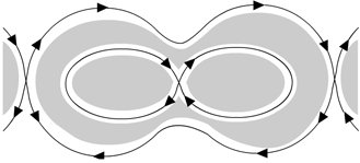
Figure 5: Phase portrait of system (4.9). Section of the oscillatory domain 𝒟0subscript𝒟0{\cal D}_{0} by {χ(Y)=const}𝜒𝑌const\{\chi(Y)=\mbox{const}\} is marked grey.
Proposition 4.1

The point χ(Y)𝜒𝑌\chi(Y) is a constant of motion in the system (P,ωP,HK0)𝑃subscript𝜔𝑃subscript𝐻superscript𝐾0(P,\omega_{P},H_{K^{0}}).

The variables λ(Y)=εp𝜆𝑌𝜀𝑝\lambda(Y)=\sqrt{\varepsilon}p and q𝑞q in the averaged system up to O(ε+λ2)𝑂𝜀superscript𝜆2O(\varepsilon+\lambda^{2}) satisfy equations (4.9).

Indeed, the first statement of Proposition 4.1 follows from the relation Y˙K0conditional˙𝑌subscript𝐾0\dot{Y}\parallel K_{0}.

Applying the operator K0,/Ysuperscript𝐾0𝑌\langle K^{0},\partial/\partial Y\rangle to (4.4) we get: K0,λY(Y)=1+O(λ)superscript𝐾0subscript𝜆𝑌𝑌1𝑂𝜆\langle K^{0},\lambda_{Y}(Y)\rangle=1+O(\lambda). Then by (4.6) in system (P,ωP,HK0)𝑃subscript𝜔𝑃subscript𝐻superscript𝐾0(P,\omega_{P},H_{K^{0}})

λ˙˙𝜆\displaystyle\dot{\lambda} =\displaystyle= λYY˙=ε𝐮q(Y,q)+O(ελ)=ε𝐡^q+O(ελ),subscriptsuperscript𝜆𝑌˙𝑌𝜀subscriptsuperscript𝐮𝑞𝑌𝑞𝑂𝜀𝜆𝜀subscriptsuperscript^𝐡𝑞𝑂𝜀𝜆\displaystyle\lambda^{\prime}_{Y}\,\dot{Y}=-\varepsilon{\bf u}^{\prime}_{q}(Y,q)+O(\varepsilon\lambda)=-\varepsilon\hat{\bf h}^{\prime}_{q}+O(\varepsilon\lambda),
q˙˙𝑞\displaystyle\dot{q} =\displaystyle= K0,HK0Y=𝒜(χ(Y))λ+O(λ2)+O(ε)=ε𝐡^p+O(ε+λ2).superscript𝐾0subscriptsuperscript𝐻superscript𝐾0𝑌𝒜𝜒𝑌𝜆𝑂superscript𝜆2𝑂𝜀𝜀subscriptsuperscript^𝐡𝑝𝑂𝜀superscript𝜆2\displaystyle\langle K^{0},H^{\prime}_{K^{0}\,Y}\rangle={\cal A}(\chi(Y))\,\lambda+O(\lambda^{2})+O(\varepsilon)=\sqrt{\varepsilon}\,\hat{\bf h}^{\prime}_{p}+O(\varepsilon+\lambda^{2}).


The projection π:U(Σ×𝕋n+1)Σ××𝕋:𝜋𝑈Σsuperscript𝕋𝑛1Σ𝕋\pi:U(\Sigma\times\mathbb{T}^{n+1})\to\Sigma\times\mathbb{R}\times\mathbb{T},

π(Y,X)=(χ(Y),p,q),p=ε1/2λ(Y),q=K0,Xformulae-sequence𝜋𝑌𝑋𝜒𝑌𝑝𝑞formulae-sequence𝑝superscript𝜀12𝜆𝑌𝑞superscript𝐾0𝑋\pi(Y,X)=(\chi(Y),p,q),\qquad p=\varepsilon^{-1/2}\lambda(Y),\quad q=\langle K^{0},X\rangle

maps the domain 𝒟ossubscript𝒟𝑜𝑠{\cal D}_{os} to 𝒟^os=π(𝒟os)subscript^𝒟𝑜𝑠𝜋subscript𝒟𝑜𝑠\hat{\cal D}_{os}=\pi({\cal D}_{os}), see Fig. 5.

Let the closed curve γ(Y,p,q)𝛾𝑌𝑝𝑞\gamma(Y,p,q) be the connected component of the set

{(p~,q~):𝐡^(χ(Y),p~,q~)=𝐡^(χ(Y),p,q)}conditional-set~𝑝~𝑞^𝐡𝜒𝑌~𝑝~𝑞^𝐡𝜒𝑌𝑝𝑞\big{\{}(\tilde{p},\tilde{q}):\hat{\bf h}(\chi(Y),\tilde{p},\tilde{q})=\hat{\bf h}(\chi(Y),p,q)\big{\}}

containing the point (p,q)𝑝𝑞(p,q). We define the action variable I𝐼I and the Hamiltonian function 𝐡𝐡{\bf h}:

I=I(Y,p,q)=12πγ(Y,p,q)p~𝑑q~,𝐡(χ(Y),I)=𝐡^(χ(Y),p,q).formulae-sequence𝐼𝐼𝑌𝑝𝑞12𝜋subscript𝛾𝑌𝑝𝑞~𝑝differential-d~𝑞𝐡𝜒𝑌𝐼^𝐡𝜒𝑌𝑝𝑞I=I(Y,p,q)=\frac{1}{2\pi}\int_{\gamma(Y,p,q)}\tilde{p}\,d\tilde{q},\qquad{\bf h}(\chi(Y),I)=\hat{\bf h}(\chi(Y),p,q). (4.10)

Note that if the energy levels 𝐡(χ(Y),p,q)=const𝐡𝜒𝑌𝑝𝑞const{\bf h}(\chi(Y),p,q)=\mbox{const} are not connected (i.e., consist of several curves γ𝛾\gamma), the function 𝐡𝐡{\bf h} is not single-valued.

If γ=γ(Y,p,q)𝛾𝛾𝑌𝑝𝑞\gamma=\gamma(Y,p,q) is a closed smooth curve, the torus

𝕋Y0,γn+1(ε)={(Y,X):χ(Y)=Y0,(ε1/2λ(Y),q)γ}superscriptsubscript𝕋superscript𝑌0𝛾𝑛1𝜀conditional-set𝑌𝑋formulae-sequence𝜒𝑌superscript𝑌0superscript𝜀12𝜆𝑌𝑞𝛾\mathbb{T}_{Y^{0},\gamma}^{n+1}(\varepsilon)=\big{\{}(Y,X):\chi(Y)=Y^{0},(\varepsilon^{-1/2}\lambda(Y),q)\in\gamma\big{\}} (4.11)

is invariant for the system (P,ωP,HK0)𝑃subscript𝜔𝑃subscript𝐻superscript𝐾0(P,\omega_{P},H_{K^{0}}) up to terms of order O(ε+λ2)𝑂𝜀superscript𝜆2O(\varepsilon+\lambda^{2}). For small ε>0𝜀0\varepsilon>0 majority of tori (4.11) survive the perturbation and exist in the original system. Any surviving torus has to satisfy several additional conditions.

(1) The frequency vector associated with 𝕋Y0,γn+1superscriptsubscript𝕋superscript𝑌0𝛾𝑛1\mathbb{T}_{Y^{0},\gamma}^{n+1} is Diophantine.

This is a standard assumption which holds on almost all tori.

(2) The system (P,ωP,HK0)𝑃subscript𝜔𝑃subscript𝐻superscript𝐾0(P,\omega_{P},H_{K^{0}}) is nondegenerate on 𝕋Y0,γn+1superscriptsubscript𝕋superscript𝑌0𝛾𝑛1\mathbb{T}_{Y^{0},\gamma}^{n+1}.

This condition essentially means that 𝐡𝐡{\bf h} is real-analytic in a neighborhood of 𝕋Y0,γn+1superscriptsubscript𝕋superscript𝑌0𝛾𝑛1\mathbb{T}_{Y^{0},\gamma}^{n+1} and

|𝐡I|<c,|𝐡II′′|<c,|𝐡I|1<c,|𝐡II|1<c.formulae-sequencesubscriptsuperscript𝐡𝐼𝑐formulae-sequencesubscriptsuperscript𝐡′′𝐼𝐼𝑐formulae-sequencesuperscriptsubscriptsuperscript𝐡𝐼1𝑐superscriptsubscriptsuperscript𝐡𝐼𝐼1𝑐|{\bf h}^{\prime}_{I}|<c,\quad|{\bf h}^{\prime\prime}_{II}|<c,\quad|{\bf h}^{\prime}_{I}|^{-1}<c,\quad|{\bf h}^{\prime}_{II}|^{-1}<c. (4.12)

Therefore we have to replace 𝒟ossubscript𝒟𝑜𝑠{\cal D}_{os} by a smaller domain 𝒟0subscript𝒟0{\cal D}_{0} by throwing out a small neighborhood of asymptotic manifolds (where the tori degenerate) and a small neighborhood of tori on which the twist conditions (4.12) is violated. Let μ𝜇\mu be the measure in the phase space 𝒟×𝕋n+1𝒟superscript𝕋𝑛1{\cal D}\times\mathbb{T}^{n+1} generated by the symplectic structure ωPsubscript𝜔𝑃\omega_{P}. Then the measures μ(𝒟)𝜇𝒟\mu({\cal D}) and μ(𝒟0)𝜇subscript𝒟0\mu({\cal D}_{0}) are both of order O(ε)𝑂𝜀O(\sqrt{\varepsilon}).

Theorem 2

Suppose that the system (P,ωP,H)𝑃subscript𝜔𝑃𝐻(P,\omega_{P},H) is real-analytic. If ε0>0subscript𝜀00\varepsilon_{0}>0 is sufficiently small, then for all positive εε0𝜀subscript𝜀0\varepsilon\leq\varepsilon_{0} any Diophantine torus 𝕋Y0,γn+1(ε)𝒟0superscriptsubscript𝕋superscript𝑌0𝛾𝑛1𝜀subscript𝒟0\mathbb{T}_{Y^{0},\gamma}^{n+1}(\varepsilon)\subset{\cal D}_{0} survives the perturbation. For some constant C>0𝐶0C>0 independent of ε𝜀\varepsilon, measure of union of such tori in 𝒟0subscript𝒟0{\cal D}_{0} is not less than μ(𝒟0)Cε𝜇subscript𝒟0𝐶𝜀\mu({\cal D}_{0})-C\varepsilon.

Remark 4.1

Note, that μ(𝒟)μ(𝒟0)εsimilar-to𝜇𝒟𝜇subscript𝒟0𝜀\mu({\cal D})-\mu({\cal D}_{0})\sim\sqrt{\varepsilon}. To obtain μ(𝒟)μ(𝒟0)εsimilar-to𝜇𝒟𝜇subscript𝒟0𝜀\mu({\cal D})-\mu({\cal D}_{0})\sim\varepsilon we need to replace in a small neighborhood of asymptotic manifolds the twist conditions (4.12) by a weaker ones. The strong proof is not ready now.

5 Preliminaries

Beginning from this place up to end of the paper we prove Theorem 2.

  • All vectors by default are regarded as columns. For any um𝑢superscript𝑚u\in\mathbb{R}^{m} and any m×m𝑚𝑚m\times m-matrix A𝐴A we use the notation

    |u|=max1jm|uj|,|A|=max0um|Au||u|.formulae-sequence𝑢subscript1𝑗𝑚subscript𝑢𝑗𝐴subscript0𝑢superscript𝑚𝐴𝑢𝑢|u|=\max_{1\leq j\leq m}|u_{j}|,\quad|A|=\max_{0\neq u\in\mathbb{R}^{m}}\frac{|Au|}{|u|}.

    The brackets ,\langle\,,\rangle denote the standard Euclidean scalar product: u,v=j=1mujvj𝑢𝑣superscriptsubscript𝑗1𝑚subscript𝑢𝑗subscript𝑣𝑗\langle u,v\rangle=\sum_{j=1}^{m}u_{j}v_{j}.

  • μ𝜇\mu denotes the standard Lebesgue measure on msuperscript𝑚\mathbb{R}^{m}.

  • Prime denotes a partial derivative e.g., fyk=f/yksubscriptsuperscript𝑓subscript𝑦𝑘𝑓subscript𝑦𝑘f^{\prime}_{y_{k}}=\partial f/\partial y_{k}. If ym𝑦superscript𝑚y\in\mathbb{R}^{m}, and f:m:𝑓superscript𝑚f:\mathbb{R}^{m}\to\mathbb{R} then fysubscriptsuperscript𝑓𝑦f^{\prime}_{y} is regarded as a vector and fyy′′subscriptsuperscript𝑓′′𝑦𝑦f^{\prime\prime}_{yy} as a matrix.

  • For any function f:𝕋m:𝑓superscript𝕋𝑚f:\mathbb{T}^{m}\to\mathbb{R} we define its average

    f=1(2π)m𝕋mf(x)𝑑x.delimited-⟨⟩𝑓1superscript2𝜋𝑚subscriptsuperscript𝕋𝑚𝑓𝑥differential-d𝑥\langle f\rangle=\frac{1}{(2\pi)^{m}}\int_{\mathbb{T}^{m}}f(x)\,dx. (5.1)

    The same notation is used if f𝑓f depends on other variables. In this case to avoid misunderstanding we use for (5.1) the notation xsubscript𝑥\langle\;\rangle_{x}.

  • Below c1,c2,subscript𝑐1subscript𝑐2c_{1},c_{2},\ldots denote positive constants. If cjsubscript𝑐𝑗c_{j} depends on another constant, say, α𝛼\alpha, we write cj(α)subscript𝑐𝑗𝛼c_{j}(\alpha). Dependence on the dimension n𝑛n is not indicated.

To present the system (P,ωP,Hg)𝑃subscript𝜔𝑃superscript𝐻𝑔(P,\omega_{P},H^{g}) in a form convenient for application of KAM procedure, we have to perform several preliminary coordinate changes.

(a). Consider a matrix MGL(n+1,)𝑀𝐺𝐿𝑛1M\in GL(n+1,\mathbb{Z}) such that K0superscript𝐾0K^{0} is its last column. In the new coordinates

Y^=M1Y,X^=MTXformulae-sequence^𝑌superscript𝑀1𝑌^𝑋superscript𝑀𝑇𝑋\hat{Y}=M^{-1}Y,\quad\hat{X}=M^{T}X

resonance (4.1) takes the form

ν^n+1(Y^)H0Y^n+1(Y^)=0,H0(Y^)=H0(Y).formulae-sequencesubscript^𝜈𝑛1^𝑌subscriptsuperscript𝐻0subscript^𝑌𝑛1^𝑌0subscript𝐻0^𝑌subscript𝐻0𝑌\hat{\nu}_{n+1}(\hat{Y})\equiv H^{\prime}_{0\,\hat{Y}_{n+1}}(\hat{Y})=0,\qquad H_{0}(\hat{Y})=H_{0}(Y). (5.2)

To have more convenient coordinates in a neighborhood of this resonance, we solve the first equation (5.2) with respect to Y^n+1subscript^𝑌𝑛1\hat{Y}_{n+1}. This can be done locally because by (4.3) H0Y^n+1Y^n+1′′0subscriptsuperscript𝐻′′0subscript^𝑌𝑛1subscript^𝑌𝑛10H^{\prime\prime}_{0\,\hat{Y}_{n+1}\hat{Y}_{n+1}}\neq 0. We denote the result

Y^n+1=G(Y^1,,Y^n),ν^n+1(Y^1,,Y^n,G(Y^1,,Y^n))0.formulae-sequencesubscript^𝑌𝑛1𝐺subscript^𝑌1subscript^𝑌𝑛subscript^𝜈𝑛1subscript^𝑌1subscript^𝑌𝑛𝐺subscript^𝑌1subscript^𝑌𝑛0\hat{Y}_{n+1}=G(\hat{Y}_{1},\ldots,\hat{Y}_{n}),\qquad\hat{\nu}_{n+1}\big{(}\hat{Y}_{1},\ldots,\hat{Y}_{n},G(\hat{Y}_{1},\ldots,\hat{Y}_{n})\big{)}\equiv 0.

(b). Consider the change of the variables

y=(y1,,yn)=(Y^1,,Y^n),p=ε1/2(Y^n+1G(y)),formulae-sequence𝑦subscript𝑦1subscript𝑦𝑛subscript^𝑌1subscript^𝑌𝑛𝑝superscript𝜀12subscript^𝑌𝑛1𝐺𝑦\displaystyle y=(y_{1},\ldots,y_{n})=(\hat{Y}_{1},\ldots,\hat{Y}_{n}),\quad p=\varepsilon^{-1/2}(\hat{Y}_{n+1}-G(y)),
x=(x1,,xn)=(X^1+Gy1q,,X^n+Gynq),q=X^n+1.formulae-sequence𝑥subscript𝑥1subscript𝑥𝑛subscript^𝑋1subscriptsuperscript𝐺subscript𝑦1𝑞subscript^𝑋𝑛subscriptsuperscript𝐺subscript𝑦𝑛𝑞𝑞subscript^𝑋𝑛1\displaystyle x=(x_{1},\ldots,x_{n})=\big{(}\hat{X}_{1}+G^{\prime}_{y_{1}}q,\ldots,\hat{X}_{n}+G^{\prime}_{y_{n}}q\big{)},\quad q=\hat{X}_{n+1}.

We are interested in motions which are oscillatory in the coordinate q𝑞q. Therefore it is not necessary to assume periodicity of this change with respect to q𝑞q. Below q𝑞q lies in an interval while the variables x𝑥x are still angular: x𝕋n𝑥superscript𝕋𝑛x\in\mathbb{T}^{n}.

The resonance ΣΣ\Sigma in the new coordinates locally takes the form {p=0}𝑝0\{p=0\}. In particular, y𝑦y are local coordinates on ΣΣ\Sigma.

Then the symplectic structure and the Hamiltonian take the form

ω=dydx+εdpdq,𝜔𝑑𝑦𝑑𝑥𝜀𝑑𝑝𝑑𝑞\displaystyle\omega=dy\wedge dx+\sqrt{\varepsilon}\,dp\wedge dq,
Λ(y)+ε(12A(y)p2+u(y,q))+εU1(y,x,q)+ε3/2U2(y,p,x,q,ε),Λ𝑦𝜀12𝐴𝑦superscript𝑝2𝑢𝑦𝑞𝜀subscript𝑈1𝑦𝑥𝑞superscript𝜀32subscript𝑈2𝑦𝑝𝑥𝑞𝜀\displaystyle\Lambda(y)+\varepsilon\big{(}\frac{1}{2}A(y)p^{2}+u(y,q)\big{)}+\varepsilon U_{1}(y,x,q)+\varepsilon^{3/2}U_{2}(y,p,x,q,\sqrt{\varepsilon}), (5.3)

where

Λ(y)=H0(y,G(y)),A(y)=H0Y^n+1Y^n+1′′(y,G(y)),formulae-sequenceΛ𝑦subscript𝐻0𝑦𝐺𝑦𝐴𝑦subscriptsuperscript𝐻′′0subscript^𝑌𝑛1subscript^𝑌𝑛1𝑦𝐺𝑦\Lambda(y)=H_{0}(y,G(y)),\quad A(y)=H^{\prime\prime}_{0\,\hat{Y}_{n+1}\hat{Y}_{n+1}}(y,G(y)),

u,U1,U2𝑢subscript𝑈1subscript𝑈2u,U_{1},U_{2} are real-analytic, and average of U1subscript𝑈1U_{1} with respect to x𝑥x vanishes: U1x=0subscriptdelimited-⟨⟩subscript𝑈1𝑥0\langle U_{1}\rangle_{x}=0.

By (4.3),(4.5)

A(y)=𝒜(χ(Y)),u(y,q)=𝐮(χ(Y),q).formulae-sequence𝐴𝑦𝒜𝜒𝑌𝑢𝑦𝑞𝐮𝜒𝑌𝑞A(y)={\cal A}\big{(}\chi(Y)\big{)},\quad u(y,q)={\bf u}(\chi(Y),q). (5.4)

Neglecting the terms εU1+ε3/2U2𝜀subscript𝑈1superscript𝜀32subscript𝑈2\varepsilon U_{1}+\varepsilon^{3/2}U_{2}, we obtain an integrable system which can be regarded as a skew-product of an n𝑛n-dimensional rotator in variables y,x𝑦𝑥y,x and a (generalized) pendulum in variables p,q𝑝𝑞p,q.

We put (see (4.7))

q^min(y)=qmin(χ(Y)),q^max(y)=qmax(χ(Y)).formulae-sequencesubscript^𝑞𝑦subscript𝑞𝜒𝑌subscript^𝑞𝑦subscript𝑞𝜒𝑌\hat{q}_{\min}(y)=q_{\min}(\chi(Y)),\quad\hat{q}_{\max}(y)=q_{\max}(\chi(Y)).

Then the domain 𝒟ossubscript𝒟𝑜𝑠{\cal D}_{os} (see (4.8)) takes the form

𝒟os={(y,p,x,q):u(y,q^min)<12A(y)p2+u(y,q)<u(y,q^max)}.subscript𝒟𝑜𝑠conditional-set𝑦𝑝𝑥𝑞𝑢𝑦subscript^𝑞12𝐴𝑦superscript𝑝2𝑢𝑦𝑞𝑢𝑦subscript^𝑞{\cal D}_{os}=\big{\{}(y,p,x,q):u(y,\hat{q}_{\min})<\frac{1}{2}A(y)p^{2}+u(y,q)<u(y,\hat{q}_{\max})\big{\}}. (5.5)

(c). Let W(y,I,q)𝑊𝑦𝐼𝑞W(y,I,q) be a generating function which introduces action-angle variables I,φ𝐼𝜑I,\varphi in domain (5.5) for the system with one degree of freedom, the symplectic structure dpdq𝑑𝑝𝑑𝑞dp\wedge dq and the Hamiltonian 12A(y)p2+u(y,q)12𝐴𝑦superscript𝑝2𝑢𝑦𝑞\frac{1}{2}A(y)p^{2}+u(y,q) for any values of the parameters y𝑦y:

p=Wq,φ=WI,h(y,I)=12A(y)p2+u(y,q).formulae-sequence𝑝subscriptsuperscript𝑊𝑞formulae-sequence𝜑subscriptsuperscript𝑊𝐼𝑦𝐼12𝐴𝑦superscript𝑝2𝑢𝑦𝑞p=W^{\prime}_{q},\quad\varphi=W^{\prime}_{I},\quad h(y,I)=\frac{1}{2}A(y)p^{2}+u(y,q).

Then the canonical change with the generating function y^x+εW(y^,I,q)^𝑦𝑥𝜀𝑊^𝑦𝐼𝑞\hat{y}x+\sqrt{\varepsilon}W(\hat{y},I,q)

y=y^,x^=x+εWy^,p=Wq,φ=WIformulae-sequence𝑦^𝑦formulae-sequence^𝑥𝑥𝜀subscriptsuperscript𝑊^𝑦formulae-sequence𝑝subscriptsuperscript𝑊𝑞𝜑subscriptsuperscript𝑊𝐼y=\hat{y},\quad\hat{x}=x+\sqrt{\varepsilon}W^{\prime}_{\hat{y}},\quad p=W^{\prime}_{q},\quad\varphi=W^{\prime}_{I}

transforms the symplectic structure to dy^dx^+εdIdφ𝑑^𝑦𝑑^𝑥𝜀𝑑𝐼𝑑𝜑d\hat{y}\wedge d\hat{x}+\sqrt{\varepsilon}dI\wedge d\varphi and Hamiltonian (5.3) to

Λ(y^)+εh(y^,I)+εV^(y^,I,x^,φ,ε),V^x=O(ε),Λ^𝑦𝜀^𝑦𝐼𝜀^𝑉^𝑦𝐼^𝑥𝜑𝜀subscriptdelimited-⟨⟩^𝑉𝑥𝑂𝜀\Lambda(\hat{y})+\varepsilon h(\hat{y},I)+\varepsilon\hat{V}(\hat{y},I,\hat{x},\varphi,\sqrt{\varepsilon}),\quad\langle\hat{V}\rangle_{x}=O(\sqrt{\varepsilon}), (5.6)

where the functions h,v^,V^=U1+εU2^𝑣^𝑉subscript𝑈1𝜀subscript𝑈2h,\hat{v},\hat{V}=U_{1}+\sqrt{\varepsilon}U_{2} are real-analytic. The function hh satisfies the equation

h(y,I)=𝐡(χ(Y),I),YU(Σ),formulae-sequence𝑦𝐼𝐡𝜒𝑌𝐼𝑌𝑈Σh(y,I)={\bf h}(\chi(Y),I),\qquad Y\in U(\Sigma),

where 𝐡𝐡{\bf h} is defined in (4.10). Below we skip hats for brevity.

6 Initial KAM Hamiltonian

For any set Dn+1𝐷superscript𝑛1D\subset\mathbb{R}^{n+1} let Ua(D)n+1subscript𝑈𝑎𝐷superscript𝑛1U_{a}(D)\subset\mathbb{C}^{n+1} be the following neighborhood:

Ua(D)={(y+η,I+ζ):(y,I)D,|η|<εa,|ζ|<a},ηn,ζ.formulae-sequencesubscript𝑈𝑎𝐷conditional-set𝑦𝜂𝐼𝜁formulae-sequence𝑦𝐼𝐷formulae-sequence𝜂𝜀𝑎𝜁𝑎formulae-sequence𝜂superscript𝑛𝜁U_{a}(D)=\{(y+\eta,I+\zeta):(y,I)\in D,|\eta|<\sqrt{\varepsilon}a,|\zeta|<a\},\qquad\eta\in\mathbb{C}^{n},\;\zeta\in\mathbb{C}.

For any function f:D:𝑓𝐷f:D\to\mathbb{R} which admits a real-analytic extension to Ua(D)subscript𝑈𝑎𝐷U_{a}(D) we put

|f|a=supzUa(D)|f(z)|.subscript𝑓𝑎subscriptsupremum𝑧subscript𝑈𝑎𝐷𝑓𝑧|f|_{a}=\sup_{z\in U_{a}(D)}|f(z)|.

Note that this norm is anisotropic in y𝑦y and I𝐼I directions.

Let Ub(𝕋n+1)subscript𝑈𝑏superscript𝕋𝑛1U_{b}(\mathbb{T}^{n+1}) be a complex neighborhood of 𝕋n+1superscript𝕋𝑛1\mathbb{T}^{n+1}

Ub(𝕋n+1)={(x+ξ,φ+κ):(x,φ)𝕋n+1,|ξ|<b,|κ|<b},ξn,κ.formulae-sequencesubscript𝑈𝑏superscript𝕋𝑛1conditional-set𝑥𝜉𝜑𝜅formulae-sequence𝑥𝜑superscript𝕋𝑛1formulae-sequence𝜉𝑏𝜅𝑏formulae-sequence𝜉superscript𝑛𝜅U_{b}(\mathbb{T}^{n+1})=\{(x+\xi,\varphi+\kappa):(x,\varphi)\in\mathbb{T}^{n+1},\,|\xi|<b,|\kappa|<b\},\qquad\xi\in\mathbb{C}^{n},\;\kappa\in\mathbb{C}.

For any function f:𝕋n+1:𝑓superscript𝕋𝑛1f:\mathbb{T}^{n+1}\to\mathbb{R} which admits a real-analytic extension to Ub(𝕋n+1)subscript𝑈𝑏superscript𝕋𝑛1U_{b}(\mathbb{T}^{n+1}) we put

|f|b=supzUb(𝕋n+1)|f(z)|.subscript𝑓𝑏subscriptsupremum𝑧subscript𝑈𝑏superscript𝕋𝑛1𝑓𝑧|f|_{b}=\sup_{z\in U_{b}(\mathbb{T}^{n+1})}|f(z)|.

For functions, real analytic on D×𝕋n+1𝐷superscript𝕋𝑛1D\times\mathbb{T}^{n+1} we define |f|a,bsubscript𝑓𝑎𝑏|f|_{a,b} as the corresponding double supremums over

Ua,b(D×𝕋n+1)=Ua(D)×Ub(𝕋n+1).subscript𝑈𝑎𝑏𝐷superscript𝕋𝑛1subscript𝑈𝑎𝐷subscript𝑈𝑏superscript𝕋𝑛1U_{a,b}(D\times\mathbb{T}^{n+1})=U_{a}(D)\times U_{b}(\mathbb{T}^{n+1}).

Consider the Hamiltonian system with the symplectic structure

dydx+εdIdφ𝑑𝑦𝑑𝑥𝜀𝑑𝐼𝑑𝜑dy\wedge dx+\sqrt{\varepsilon}\,dI\wedge d\varphi (6.1)

and the real-analytic Hamiltonian (see (5.6))

H0=Λ(y)+εh0(y,I)+εv0(y,I,φ,ε)+εu0(y,I,x,φ,ε),v0(y,I,φ,0)=0,u0x=0,formulae-sequencesubscript𝐻0Λ𝑦𝜀subscript0𝑦𝐼𝜀subscript𝑣0𝑦𝐼𝜑𝜀𝜀subscript𝑢0𝑦𝐼𝑥𝜑𝜀formulae-sequencesubscript𝑣0𝑦𝐼𝜑00subscriptdelimited-⟨⟩subscript𝑢0𝑥0H_{0}=\Lambda(y)+\varepsilon h_{0}(y,I)+\varepsilon v_{0}(y,I,\varphi,\sqrt{\varepsilon})+\varepsilon u_{0}(y,I,x,\varphi,\sqrt{\varepsilon}),\qquad v_{0}(y,I,\varphi,0)=0,\quad\langle u_{0}\rangle_{x}=0,

where v0=Vxsubscript𝑣0subscriptdelimited-⟨⟩𝑉𝑥v_{0}=\langle V\rangle_{x}, u0=VVxsubscript𝑢0𝑉subscriptdelimited-⟨⟩𝑉𝑥u_{0}=V-\langle V\rangle_{x} and the points (y,I,x,φ)𝑦𝐼𝑥𝜑(y,I,x,\varphi) lie in a complex neighborhood

Ua0,b0(D0×𝕋n+1),D0n+1subscript𝑈subscript𝑎0subscript𝑏0subscript𝐷0superscript𝕋𝑛1subscript𝐷0superscript𝑛1U_{a_{0},b_{0}}(D_{0}\times\mathbb{T}^{n+1}),\qquad D_{0}\subset\mathbb{R}^{n+1}

for some a0,b0>0subscript𝑎0subscript𝑏00a_{0},b_{0}>0.

The above analyticity assumptions mean that there exist ε0,s¯0,s0>0subscript𝜀0subscript¯𝑠0subscript𝑠00\varepsilon_{0},\bar{s}_{0},s_{0}>0 such that for any 0ε<ε00𝜀subscript𝜀00\leq\varepsilon<\varepsilon_{0}

|Λ|a0s¯0,|h0|a0ch,|u0|a0,b0s0,|v0|a0,b0ε𝐜.formulae-sequencesubscriptΛsubscript𝑎0subscript¯𝑠0formulae-sequencesubscriptsubscript0subscript𝑎0subscript𝑐formulae-sequencesubscriptsubscript𝑢0subscript𝑎0subscript𝑏0subscript𝑠0subscriptsubscript𝑣0subscript𝑎0subscript𝑏0𝜀𝐜|\Lambda|_{a_{0}}\leq\bar{s}_{0},\quad|h_{0}|_{a_{0}}\leq c_{h},\quad|u_{0}|_{a_{0},b_{0}}\leq s_{0},\quad|v_{0}|_{a_{0},b_{0}}\leq\sqrt{\varepsilon}{\bf c}. (6.2)

Assumptions of Theorem 2 imply the following non-degeneracy conditions:

c¯Λ|detΛyy′′|c¯Λ,|Λyy′′|a0cΛ,|Λyy′′1|a0cΛ,|h0I|a0ch,|h0I|a01ch,formulae-sequencesubscript¯𝑐ΛsubscriptsuperscriptΛ′′𝑦𝑦subscript¯𝑐Λformulae-sequencesubscriptsubscriptsuperscriptΛ′′𝑦𝑦subscript𝑎0subscript𝑐Λformulae-sequencesubscriptsubscriptsuperscriptΛ′′1𝑦𝑦subscript𝑎0subscript𝑐Λformulae-sequencesubscriptsubscriptsuperscript0𝐼subscript𝑎0subscriptsuperscript𝑐subscriptsuperscriptsubscriptsuperscript0𝐼1subscript𝑎0subscriptsuperscript𝑐\displaystyle\!\!\!\!\!\!\underline{c}_{\Lambda}\leq|\det\Lambda^{\prime\prime}_{yy}|\leq\overline{c}_{\Lambda},\quad|\Lambda^{\prime\prime}_{yy}|_{a_{0}}\leq c_{\Lambda},\quad|\Lambda^{\prime\prime\,-1}_{yy}|_{a_{0}}\leq c_{\Lambda},\quad|h^{\prime}_{0\,I}|_{a_{0}}\leq c^{\prime}_{h},\quad|h^{\prime}_{0\,I}|^{-1}_{a_{0}}\leq c^{\prime}_{h},\quad (6.3)
|h0II′′|a0ch,|h0II′′|a01ch,|εh0Iy′′|a0ch′′,|εh0yy′′|a0ch′′.formulae-sequencesubscriptsubscriptsuperscript′′0𝐼𝐼subscript𝑎0subscriptsuperscript𝑐formulae-sequencesubscriptsuperscriptsubscriptsuperscript′′0𝐼𝐼1subscript𝑎0subscriptsuperscript𝑐formulae-sequencesubscript𝜀subscriptsuperscript′′0𝐼𝑦subscript𝑎0subscriptsuperscript𝑐′′subscript𝜀subscriptsuperscript′′0𝑦𝑦subscript𝑎0subscriptsuperscript𝑐′′\displaystyle\!\!\!\!\!\!|h^{\prime\prime}_{0\,II}|_{a_{0}}\leq c^{\prime}_{h},\quad|h^{\prime\prime}_{0\,II}|^{-1}_{a_{0}}\leq c^{\prime}_{h},\quad|\sqrt{\varepsilon}h^{\prime\prime}_{0\,Iy}|_{a_{0}}\leq c^{\prime\prime}_{h},\quad|\varepsilon h^{\prime\prime}_{0\,yy}|_{a_{0}}\leq c^{\prime\prime}_{h}. (6.4)

Let ε𝜀\varepsilon be sufficiently small, then we can assume that ch′′subscriptsuperscript𝑐′′c^{\prime\prime}_{h} is small because ch′′εsimilar-tosubscriptsuperscript𝑐′′𝜀c^{\prime\prime}_{h}\sim\sqrt{\varepsilon}. Below we assume that ch′′ch 0′′(c¯Λ,cΛ,ch)subscriptsuperscript𝑐′′subscriptsuperscript𝑐′′ 0subscript¯𝑐Λsubscript𝑐Λsubscriptsuperscript𝑐c^{\prime\prime}_{h}\leq c^{\prime\prime}_{h\,0}(\underline{c}_{\Lambda},c_{\Lambda},c^{\prime}_{h}).

7 The Hamiltonian Hmsubscript𝐻𝑚H_{m}

Below all functions depend smoothly on ε𝜀\varepsilon. For brevity we do not write ε𝜀\varepsilon in their arguments.

As usual KAM procedure includes a converging sequence 0,1,subscript0subscript1{\cal F}_{0},{\cal F}_{1},\ldots of coordinate changes and a converging sequence of Hamiltonians H0,H1,subscript𝐻0subscript𝐻1H_{0},H_{1},\ldots

m:Uam+1,bm+1(Dm+1×𝕋n+1)Uam,bm(Dm×𝕋n+1),Hm+1=Hmm.:subscript𝑚formulae-sequencesubscript𝑈subscript𝑎𝑚1subscript𝑏𝑚1subscript𝐷𝑚1superscript𝕋𝑛1subscript𝑈subscript𝑎𝑚subscript𝑏𝑚subscript𝐷𝑚superscript𝕋𝑛1subscript𝐻𝑚1subscript𝐻𝑚subscript𝑚{\cal F}_{m}:U_{a_{m+1},b_{m+1}}(D_{m+1}\times\mathbb{T}^{n+1})\to U_{a_{m},b_{m}}(D_{m}\times\mathbb{T}^{n+1}),\quad H_{m+1}=H_{m}\circ{\cal F}_{m}.

Consider an increasing sequence {Nj}subscript𝑁𝑗\{N_{j}\in\mathbb{Z}\} (Njsubscript𝑁𝑗N_{j} is the maximal order of a resonance essential on the j𝑗j-th step), a decreasing sequence {λj>0}subscript𝜆𝑗0\{\lambda_{j}>0\} (ελj𝜀subscript𝜆𝑗\sqrt{\varepsilon}\,\lambda_{j} determines the width of resonance strips on the j𝑗j-th step) and the function 𝐣::𝐣{\bf j}:\mathbb{N}\to\mathbb{N} defined by the inequality (let N1=0subscript𝑁10N_{-1}=0)

N𝐣(r)1<rN𝐣(r)for all r>0.formulae-sequencesubscript𝑁𝐣𝑟1𝑟subscript𝑁𝐣𝑟for all r>0N_{{\bf j}(r)-1}<r\leq N_{{\bf j}(r)}\quad\mbox{for all $r>0$}. (7.1)

Then 𝐣(r)𝐣𝑟{\bf j}(r) is the number of the first step on which the resonance of order r𝑟r is essential.

Consider two positive decreasing sequences am,bmsubscript𝑎𝑚subscript𝑏𝑚a_{m},b_{m},

am=am+1+6σm,bm=bm+1+3δmformulae-sequencesubscript𝑎𝑚subscript𝑎𝑚16subscript𝜎𝑚subscript𝑏𝑚subscript𝑏𝑚13subscript𝛿𝑚a_{m}=a_{m+1}+6\sigma_{m},\quad b_{m}=b_{m+1}+3\delta_{m} (7.2)

Suppose that on the m𝑚m-th step we have the Hamiltonian

Hm=Λ(y)+εhm(y,I)+εvm(y,I,φ)+εum(y,I,x,φ),umx=0.formulae-sequencesubscript𝐻𝑚Λ𝑦𝜀subscript𝑚𝑦𝐼𝜀subscript𝑣𝑚𝑦𝐼𝜑𝜀subscript𝑢𝑚𝑦𝐼𝑥𝜑subscriptdelimited-⟨⟩subscript𝑢𝑚𝑥0H_{m}=\Lambda(y)+\varepsilon h_{m}(y,I)+\varepsilon v_{m}(y,I,\varphi)+\varepsilon u_{m}(y,I,x,\varphi),\qquad\langle u_{m}\rangle_{x}=0. (7.3)

The function Hmsubscript𝐻𝑚H_{m} is defined in a complex neighborhood Uam,bm(Dm×𝕋n+1)subscript𝑈subscript𝑎𝑚subscript𝑏𝑚subscript𝐷𝑚superscript𝕋𝑛1U_{a_{m},b_{m}}(D_{m}\times\mathbb{T}^{n+1})

Dm+1=Dm|K|Nm,k0Uam(QK,m),K=(kk0)n+1,kn,formulae-sequenceformulae-sequencesubscript𝐷𝑚1subscript𝐷𝑚subscriptformulae-sequence𝐾subscript𝑁𝑚𝑘0subscript𝑈subscript𝑎𝑚subscript𝑄𝐾𝑚𝐾𝑘subscript𝑘0superscript𝑛1𝑘superscript𝑛D_{m+1}=D_{m}\setminus\bigcup_{|K|\leq N_{m},\,k\neq 0}U_{a_{m}}(Q_{K,m}),\qquad K=\Big{(}\begin{array}[]{c}k\\ k_{0}\end{array}\Big{)}\in\mathbb{Z}^{n+1},\quad k\in\mathbb{Z}^{n}, (7.4)

where the resonant strips QK,msubscript𝑄𝐾𝑚Q_{K,m} are defined with the help of the sequences Njsubscript𝑁𝑗N_{j} and λjsubscript𝜆𝑗\lambda_{j}:

QK,m={(y,I)Uam(Dm):|νm(y,I),K|λ𝐣(|K|)(1+2m1)ε},subscript𝑄𝐾𝑚conditional-set𝑦𝐼subscript𝑈subscript𝑎𝑚subscript𝐷𝑚subscript𝜈𝑚𝑦𝐼𝐾subscript𝜆𝐣𝐾1superscript2𝑚1𝜀\displaystyle Q_{K,m}=\big{\{}(y,I)\in U_{a_{m}}(D_{m}):\big{|}\langle\nu_{m}(y,I),K\rangle\big{|}\leq\lambda_{{\bf j}(|K|)}(1+2^{-m-1})\sqrt{\varepsilon}\big{\}}, (7.5)
νm(y,I)=(Λy(y)+εhmy(y,I)εhmI(y,I)).subscript𝜈𝑚𝑦𝐼subscriptsuperscriptΛ𝑦𝑦𝜀subscriptsuperscript𝑚𝑦𝑦𝐼𝜀subscriptsuperscript𝑚𝐼𝑦𝐼\displaystyle\nu_{m}(y,I)=\Big{(}\begin{array}[]{c}\Lambda^{\prime}_{y}(y)+\varepsilon h^{\prime}_{m\,y}(y,I)\\ \sqrt{\varepsilon}\,h^{\prime}_{m\,I}(y,I)\end{array}\Big{)}. (7.8)
Proposition 7.1

For any m=1,2,𝑚12m=1,2,\ldots

μ(D0Dm)cμε,𝜇subscript𝐷0subscript𝐷𝑚subscript𝑐𝜇𝜀\mu(D_{0}\setminus D_{m})\leq c_{\mu}\sqrt{\varepsilon},

where cμ>0subscript𝑐𝜇0c_{\mu}>0 is independent of ε𝜀\varepsilon.

Inductive assumptions. For (y,I)Uam(Dm)𝑦𝐼subscript𝑈subscript𝑎𝑚subscript𝐷𝑚(y,I)\in U_{a_{m}}(D_{m}) the following estimates hold:

|vm|am,bmsm,|um|am,bmsm,formulae-sequencesubscriptsubscript𝑣𝑚subscript𝑎𝑚subscript𝑏𝑚subscript𝑠𝑚subscriptsubscript𝑢𝑚subscript𝑎𝑚subscript𝑏𝑚subscript𝑠𝑚\displaystyle|v_{m}|_{a_{m},b_{m}}\leq s_{m},\quad|u_{m}|_{a_{m},b_{m}}\leq s_{m}, (7.9)
|hm|am(22m)ch,|hmI|am1(22m)ch,|hmII′′|am1(22m)ch,formulae-sequencesubscriptsubscript𝑚subscript𝑎𝑚2superscript2𝑚subscript𝑐formulae-sequencesuperscriptsubscriptsubscriptsuperscript𝑚𝐼subscript𝑎𝑚12superscript2𝑚subscriptsuperscript𝑐superscriptsubscriptsubscriptsuperscript′′𝑚𝐼𝐼subscript𝑎𝑚12superscript2𝑚subscriptsuperscript𝑐\displaystyle|h_{m}|_{a_{m}}\leq(2-2^{-m})c_{h},\quad|h^{\prime}_{m\,I}|_{a_{m}}^{-1}\leq(2-2^{-m})c^{\prime}_{h},\quad|h^{\prime\prime}_{m\,II}|_{a_{m}}^{-1}\leq(2-2^{-m})c^{\prime}_{h}, (7.10)
|hmII′′|am(22m)ch,|εhmIy′′|am(22m)ch′′,|εhmyy′′|am(22m)ch′′.formulae-sequencesubscriptsubscriptsuperscript′′𝑚𝐼𝐼subscript𝑎𝑚2superscript2𝑚subscriptsuperscript𝑐formulae-sequencesubscript𝜀subscriptsuperscript′′𝑚𝐼𝑦subscript𝑎𝑚2superscript2𝑚subscriptsuperscript𝑐′′subscript𝜀subscriptsuperscript′′𝑚𝑦𝑦subscript𝑎𝑚2superscript2𝑚subscriptsuperscript𝑐′′\displaystyle\displaystyle|h^{\prime\prime}_{m\,II}|_{a_{m}}\leq(2-2^{-m})c^{\prime}_{h},\quad|\sqrt{\varepsilon}h^{\prime\prime}_{m\,Iy}|_{a_{m}}\leq(2-2^{-m})c^{\prime\prime}_{h},\quad|\varepsilon h^{\prime\prime}_{m\,yy}|_{a_{m}}\leq(2-2^{-m})c^{\prime\prime}_{h}. (7.11)

8 The KAM-step

For any natural N𝑁N and a periodic function

f:𝕋n+1,f(x,φ)=K=(k,k0)n+1fKeik,x+ik0φ:𝑓formulae-sequencesuperscript𝕋𝑛1𝑓𝑥𝜑subscript𝐾𝑘subscript𝑘0superscript𝑛1superscript𝑓𝐾superscript𝑒𝑖𝑘𝑥𝑖subscript𝑘0𝜑f:\mathbb{T}^{n+1}\to\mathbb{R},\qquad f(x,\varphi)=\sum_{K=(k,k_{0})\in\mathbb{Z}^{n+1}}f^{K}e^{i\langle k,x\rangle+ik_{0}\varphi}

we define the cut off

ΠNf(x,φ)=|K|N,k0fKeik,x+ik0φ.subscriptΠ𝑁𝑓𝑥𝜑subscriptformulae-sequence𝐾𝑁𝑘0superscript𝑓𝐾superscript𝑒𝑖𝑘𝑥𝑖subscript𝑘0𝜑\Pi_{N}f(x,\varphi)=\sum_{|K|\leq N,\,k\neq 0}f^{K}e^{i\langle k,x\rangle+ik_{0}\varphi}. (8.1)

Then by Lemma 12.1 for any real-analytic f𝑓f such that |f|b<subscript𝑓𝑏|f|_{b}<\infty and for any δ(0,b)𝛿0𝑏\delta\in(0,b)

|ffxΠNf|bδCδ(N+1δ)neNδ|f|b.subscript𝑓subscriptdelimited-⟨⟩𝑓𝑥subscriptΠ𝑁𝑓𝑏𝛿𝐶𝛿superscript𝑁1𝛿𝑛superscript𝑒𝑁𝛿subscript𝑓𝑏\big{|}f-\langle f\rangle_{x}-\Pi_{N}f\big{|}_{b-\delta}\leq\frac{C}{\delta}\Big{(}N+\frac{1}{\delta}\Big{)}^{n}e^{-N\delta}\,|f|_{b}. (8.2)

By using Hamiltonian (7.3), we introduce the canonical666i.e., preserving symplectic structure (6.1) change of variables (y,I,x,φ)(y^,I^,x^,φ^)maps-to𝑦𝐼𝑥𝜑^𝑦^𝐼^𝑥^𝜑(y,I,x,\varphi)\mapsto(\hat{y},\hat{I},\hat{x},\hat{\varphi}), determined by the generating function y^x+ε(I^φ+S(y^,I^,x,φ))^𝑦𝑥𝜀^𝐼𝜑𝑆^𝑦^𝐼𝑥𝜑\hat{y}x+\sqrt{\varepsilon}\big{(}\hat{I}\varphi+S(\hat{y},\hat{I},x,\varphi)\big{)}:

y=y^+εSx,I=I^+Sφ,x^=x+εSy^,φ^=φ+SI^,formulae-sequence𝑦^𝑦𝜀subscriptsuperscript𝑆𝑥formulae-sequence𝐼^𝐼subscriptsuperscript𝑆𝜑formulae-sequence^𝑥𝑥𝜀subscriptsuperscript𝑆^𝑦^𝜑𝜑subscriptsuperscript𝑆^𝐼y=\hat{y}+\sqrt{\varepsilon}S^{\prime}_{x},\quad I=\hat{I}+S^{\prime}_{\varphi},\quad\hat{x}=x+\sqrt{\varepsilon}S^{\prime}_{\hat{y}},\quad\hat{\varphi}=\varphi+S^{\prime}_{\hat{I}},

where the arguments (y^,I^)^𝑦^𝐼(\hat{y},\hat{I}) are supposed to lie in Uamσm(Dm+1)subscript𝑈subscript𝑎𝑚subscript𝜎𝑚subscript𝐷𝑚1U_{a_{m}-\sigma_{m}}(D_{m+1}).

Remark 8.1

||amσ,bmδ|\cdot|_{a_{m}-\sigma,b_{m}-\delta} (resp. ||amσ|\cdot|_{a_{m}-\sigma}) denotes the norm in Uamσ,bmδ(Dm+1×𝕋n+1)subscript𝑈subscript𝑎𝑚𝜎subscript𝑏𝑚𝛿subscript𝐷𝑚1superscript𝕋𝑛1U_{a_{m}-\sigma,b_{m}-\delta}(D_{m+1}\times\mathbb{T}^{n+1}) (resp. Uamσ(Dm+1)subscript𝑈subscript𝑎𝑚𝜎subscript𝐷𝑚1U_{a_{m}-\sigma}(D_{m+1})).

By definition the function S𝑆S is a solution of the homological equation

νm(y^,I^),(SxSφ)(y^,I^,x,φ)=εΠNmVm(y^,I^,x,φ),Vm=vm+um.formulae-sequencesubscript𝜈𝑚^𝑦^𝐼subscriptsuperscript𝑆𝑥subscriptsuperscript𝑆𝜑^𝑦^𝐼𝑥𝜑𝜀subscriptΠsubscript𝑁𝑚subscript𝑉𝑚^𝑦^𝐼𝑥𝜑subscript𝑉𝑚subscript𝑣𝑚subscript𝑢𝑚\Big{\langle}\nu_{m}(\hat{y},\hat{I}),\Big{(}\!\!\begin{array}[]{c}S^{\prime}_{x}\\ S^{\prime}_{\varphi}\end{array}\!\!\Big{)}(\hat{y},\hat{I},x,\varphi)\Big{\rangle}=-\sqrt{\varepsilon}\,\Pi_{N_{m}}V_{m}(\hat{y},\hat{I},x,\varphi),\qquad V_{m}=v_{m}+u_{m}. (8.3)
Proposition 8.1

For any m=0,1,𝑚01m=0,1,\ldots there exists a solution of (8.3) where

|S|am,bmδmLmsm,Lm=j=0m2Njn+1λje(n+1)δmNj1.formulae-sequencesubscript𝑆subscript𝑎𝑚subscript𝑏𝑚subscript𝛿𝑚subscript𝐿𝑚subscript𝑠𝑚subscript𝐿𝑚superscriptsubscript𝑗0𝑚2superscriptsubscript𝑁𝑗𝑛1subscript𝜆𝑗superscript𝑒𝑛1subscript𝛿𝑚subscript𝑁𝑗1|S|_{a_{m},b_{m}-\delta_{m}}\leq L_{m}s_{m},\qquad L_{m}=\sum_{j=0}^{m}2\frac{N_{j}^{n+1}}{\lambda_{j}}e^{-(n+1)\delta_{m}N_{j-1}}. (8.4)

The Hamiltonian (7.3) takes the form

H~m=Λ(y^)+εhm(y^,I^)+εvm(y^,I^,φ^)+εv~m(y^,I^,φ^)+εu~m(y^,I^,x^,φ^),u~mx=0.formulae-sequencesubscript~𝐻𝑚Λ^𝑦𝜀subscript𝑚^𝑦^𝐼𝜀subscript𝑣𝑚^𝑦^𝐼^𝜑𝜀subscript~𝑣𝑚^𝑦^𝐼^𝜑𝜀subscript~𝑢𝑚^𝑦^𝐼^𝑥^𝜑subscriptdelimited-⟨⟩subscript~𝑢𝑚𝑥0\widetilde{H}_{m}=\Lambda(\hat{y})+\varepsilon h_{m}(\hat{y},\hat{I})+\varepsilon v_{m}(\hat{y},\hat{I},\hat{\varphi})+\varepsilon\tilde{v}_{m}(\hat{y},\hat{I},\hat{\varphi})+\varepsilon\tilde{u}_{m}(\hat{y},\hat{I},\hat{x},\hat{\varphi}),\qquad\langle\tilde{u}_{m}\rangle_{x}=0. (8.5)
Remark 8.2

Below we show that that

|Sx|amσm,bm2δmσm,|Sφ|amσm,bm2δmσm,formulae-sequencesubscriptsubscriptsuperscript𝑆𝑥subscript𝑎𝑚subscript𝜎𝑚subscript𝑏𝑚2subscript𝛿𝑚subscript𝜎𝑚subscriptsubscriptsuperscript𝑆𝜑subscript𝑎𝑚subscript𝜎𝑚subscript𝑏𝑚2subscript𝛿𝑚subscript𝜎𝑚\displaystyle|S^{\prime}_{x}|_{a_{m}-\sigma_{m},b_{m}-2\delta_{m}}\leq\sigma_{m},\quad|S^{\prime}_{\varphi}|_{a_{m}-\sigma_{m},b_{m}-2\delta_{m}}\leq\sigma_{m}, (8.6)
|εSy|amσm,bm2δmδm,|SI|amσm,bm2δmδm.formulae-sequencesubscript𝜀subscriptsuperscript𝑆𝑦subscript𝑎𝑚subscript𝜎𝑚subscript𝑏𝑚2subscript𝛿𝑚subscript𝛿𝑚subscriptsubscriptsuperscript𝑆𝐼subscript𝑎𝑚subscript𝜎𝑚subscript𝑏𝑚2subscript𝛿𝑚subscript𝛿𝑚\displaystyle|\sqrt{\varepsilon}S^{\prime}_{y}|_{a_{m}-\sigma_{m},b_{m}-2\delta_{m}}\leq\delta_{m},\quad|S^{\prime}_{I}|_{a_{m}-\sigma_{m},b_{m}-2\delta_{m}}\leq\delta_{m}. (8.7)

Estimates (8.6)–(8.7) imply that the coordinate change is well-defined for (y^,I^,x^,φ^)Uamσm,bm2δm(Dm+1×𝕋n+1)^𝑦^𝐼^𝑥^𝜑subscript𝑈subscript𝑎𝑚subscript𝜎𝑚subscript𝑏𝑚2subscript𝛿𝑚subscript𝐷𝑚1superscript𝕋𝑛1(\hat{y},\hat{I},\hat{x},\hat{\varphi})\in U_{a_{m}-\sigma_{m},b_{m}-2\delta_{m}}(D_{m+1}\times\mathbb{T}^{n+1}).

Proposition 8.2

For m1𝑚1m\geq 1 estimates (8.6)–(8.7) imply the inequalities

|v~m+u~m|amσm,bm2δms~m,subscriptsubscript~𝑣𝑚subscript~𝑢𝑚subscript𝑎𝑚subscript𝜎𝑚subscript𝑏𝑚2subscript𝛿𝑚subscript~𝑠𝑚\displaystyle|\tilde{v}_{m}+\tilde{u}_{m}|_{a_{m}-\sigma_{m},b_{m}-2\delta_{m}}\leq\tilde{s}_{m}, (8.8)
s~m=(cΛ+ch)(Lmsmδm)2+(n+2)Lmsm2σmδm+Cδm(Nm+1δm)neNmδmsm.subscript~𝑠𝑚subscript𝑐Λsubscriptsuperscript𝑐superscriptsubscript𝐿𝑚subscript𝑠𝑚subscript𝛿𝑚2𝑛2subscript𝐿𝑚superscriptsubscript𝑠𝑚2subscript𝜎𝑚subscript𝛿𝑚𝐶subscript𝛿𝑚superscriptsubscript𝑁𝑚1subscript𝛿𝑚𝑛superscript𝑒subscript𝑁𝑚subscript𝛿𝑚subscript𝑠𝑚\displaystyle\displaystyle{\tilde{s}_{m}=(c_{\Lambda}+c^{\prime}_{h})\Big{(}\frac{L_{m}s_{m}}{\delta_{m}}\Big{)}^{2}+(n+2)\frac{L_{m}s_{m}^{2}}{\sigma_{m}\delta_{m}}+\frac{C}{\delta_{m}}\Big{(}N_{m}+\frac{1}{\delta_{m}}\Big{)}^{n}e^{-N_{m}\delta_{m}}\,s_{m}}. (8.9)

9 An additional step

Consider the symplectic transformation (I^,φ^)(I¯,φ¯)maps-to^𝐼^𝜑¯𝐼¯𝜑(\hat{I},\hat{\varphi})\mapsto(\bar{I},\bar{\varphi}) with generating function I¯φ^+εS~(y¯,I¯,φ^)¯𝐼^𝜑𝜀~𝑆¯𝑦¯𝐼^𝜑\bar{I}\hat{\varphi}+\sqrt{\varepsilon}\widetilde{S}(\bar{y},\bar{I},\hat{\varphi}) which introduces action-angle variables in the system with one degree of freedom and Hamiltonian

hm(y^,I^)+vm(y^,I^,φ^)=hm+1(y¯,I¯).subscript𝑚^𝑦^𝐼subscript𝑣𝑚^𝑦^𝐼^𝜑subscript𝑚1¯𝑦¯𝐼h_{m}(\hat{y},\hat{I})+v_{m}(\hat{y},\hat{I},\hat{\varphi})=h_{m+1}(\bar{y},\bar{I}). (9.1)

The variables y^=y¯^𝑦¯𝑦\hat{y}=\bar{y} are regarded as parameters. We extend this map to a canonical transformation of the whole phase space:

y^=y¯,I^=I¯+S~φ^,x¯=x^+εS~y¯,φ¯=φ^+S~I¯.formulae-sequence^𝑦¯𝑦formulae-sequence^𝐼¯𝐼subscriptsuperscript~𝑆^𝜑formulae-sequence¯𝑥^𝑥𝜀subscriptsuperscript~𝑆¯𝑦¯𝜑^𝜑subscriptsuperscript~𝑆¯𝐼\hat{y}=\bar{y},\quad\hat{I}=\bar{I}+\widetilde{S}^{\prime}_{\hat{\varphi}},\quad\bar{x}=\hat{x}+\sqrt{\varepsilon}\widetilde{S}^{\prime}_{\bar{y}},\quad\bar{\varphi}=\hat{\varphi}+\widetilde{S}^{\prime}_{\bar{I}}. (9.2)

Then Hamiltonian (8.5) takes the form

Hm+1=Λ(y¯)+εhm+1(y¯,I¯)+εvm+1(y¯,I¯,φ¯)+εum+1(y¯,I¯,x¯,φ¯),um+1x¯=0.formulae-sequencesubscript𝐻𝑚1Λ¯𝑦𝜀subscript𝑚1¯𝑦¯𝐼𝜀subscript𝑣𝑚1¯𝑦¯𝐼¯𝜑𝜀subscript𝑢𝑚1¯𝑦¯𝐼¯𝑥¯𝜑subscriptdelimited-⟨⟩subscript𝑢𝑚1¯𝑥0H_{m+1}=\Lambda(\bar{y})+\varepsilon h_{m+1}(\bar{y},\bar{I})+\varepsilon v_{m+1}(\bar{y},\bar{I},\bar{\varphi})+\varepsilon u_{m+1}(\bar{y},\bar{I},\bar{x},\bar{\varphi}),\qquad\langle u_{m+1}\rangle_{\bar{x}}=0.
Proposition 9.1

Suppose that

|v0|a0ε𝐜σ0δ02ch,|vm|amσm,bm2δmsm,smσmδm4ch,m1.formulae-sequencesubscriptsubscript𝑣0subscript𝑎0𝜀𝐜subscript𝜎0subscript𝛿02subscriptsuperscript𝑐formulae-sequencesubscriptsubscript𝑣𝑚subscript𝑎𝑚subscript𝜎𝑚subscript𝑏𝑚2subscript𝛿𝑚subscript𝑠𝑚formulae-sequencesubscript𝑠𝑚subscript𝜎𝑚subscript𝛿𝑚4subscriptsuperscript𝑐𝑚1|v_{0}|_{a_{0}}\leq\sqrt{\varepsilon}{\bf c}\leq\frac{\sigma_{0}\delta_{0}}{2c^{\prime}_{h}},\quad|v_{m}|_{a_{m}-\sigma_{m},b_{m}-2\delta_{m}}\leq s_{m},\quad s_{m}\leq\frac{\sigma_{m}\delta_{m}}{4c^{\prime}_{h}},\qquad m\geq 1. (9.3)

Then for any m0𝑚0m\geq 0

|S~φ^|am4σm,bm2δm8chsm,|S~|am4σm,bm2δm16πchsm,formulae-sequencesubscriptsubscriptsuperscript~𝑆^𝜑subscript𝑎𝑚4subscript𝜎𝑚subscript𝑏𝑚2subscript𝛿𝑚8subscriptsuperscript𝑐subscriptsuperscript𝑠𝑚subscript~𝑆subscript𝑎𝑚4subscript𝜎𝑚subscript𝑏𝑚2subscript𝛿𝑚16𝜋subscriptsuperscript𝑐subscriptsuperscript𝑠𝑚\displaystyle|\tilde{S}^{\prime}_{\hat{\varphi}}|_{a_{m}-4\sigma_{m},b_{m}-2\delta_{m}}\leq 8c^{\prime}_{h}s^{\prime}_{m},\quad|\tilde{S}|_{a_{m}-4\sigma_{m},b_{m}-2\delta_{m}}\leq 16\pi c^{\prime}_{h}s^{\prime}_{m}, (9.4)
|hm+1hm|am4σm,bm2δm8chchsmσm,|um+1+vm+1|am+1,bm+1sm,formulae-sequencesubscriptsubscript𝑚1subscript𝑚subscript𝑎𝑚4subscript𝜎𝑚subscript𝑏𝑚2subscript𝛿𝑚8subscript𝑐subscriptsuperscript𝑐subscriptsuperscript𝑠𝑚subscript𝜎𝑚subscriptsubscript𝑢𝑚1subscript𝑣𝑚1subscript𝑎𝑚1subscript𝑏𝑚1subscriptsuperscript𝑠𝑚\displaystyle|h_{m+1}-h_{m}|_{a_{m}-4\sigma_{m},b_{m}-2\delta_{m}}\leq\frac{8c_{h}c^{\prime}_{h}s^{\prime}_{m}}{\sigma_{m}},\quad|u_{m+1}+v_{m+1}|_{a_{m+1},b_{m+1}}\leq s^{\prime}_{m}, (9.5)

where s0=ε𝐜subscriptsuperscript𝑠0𝜀𝐜s^{\prime}_{0}=\sqrt{\varepsilon}{\bf c} and sm=smsubscriptsuperscript𝑠𝑚subscript𝑠𝑚s^{\prime}_{m}=s_{m} for all m1𝑚1m\geq 1.

Remark 9.1

Below we show that

|S~I¯|am+1,bm+1δm,|εS~y¯|am+1,bm+1δm,formulae-sequencesubscriptsubscriptsuperscript~𝑆¯𝐼subscript𝑎𝑚1subscript𝑏𝑚1subscript𝛿𝑚subscript𝜀subscriptsuperscript~𝑆¯𝑦subscript𝑎𝑚1subscript𝑏𝑚1subscript𝛿𝑚\displaystyle|\widetilde{S}^{\prime}_{\bar{I}}|_{a_{m+1},b_{m+1}}\leq\delta_{m},\quad|\sqrt{\varepsilon}\widetilde{S}^{\prime}_{\bar{y}}|_{a_{m+1},b_{m+1}}\leq\delta_{m}, (9.6)
|S~φ^|am+1,bm+1σm.subscriptsubscriptsuperscript~𝑆^𝜑subscript𝑎𝑚1subscript𝑏𝑚1subscript𝜎𝑚\displaystyle|\widetilde{S}^{\prime}_{\hat{\varphi}}|_{a_{m+1},b_{m+1}}\leq\sigma_{m}. (9.7)

Estimates (9.6),(9.7) imply that the coordinate change (9.2) is well-defined for (y¯,I¯,x¯,φ¯)Uam+1,bm+1(Dm+1×𝕋n+1)¯𝑦¯𝐼¯𝑥¯𝜑subscript𝑈subscript𝑎𝑚1subscript𝑏𝑚1subscript𝐷𝑚1superscript𝕋𝑛1(\bar{y},\bar{I},\bar{x},\bar{\varphi})\in U_{a_{m+1},b_{m+1}}(D_{m+1}\times\mathbb{T}^{n+1}).

10 The sequences σm,δm,sm,Lm,Nm,λmsubscript𝜎𝑚subscript𝛿𝑚subscript𝑠𝑚subscript𝐿𝑚subscript𝑁𝑚subscript𝜆𝑚\sigma_{m},\delta_{m},s_{m},L_{m},N_{m},\lambda_{m}

We define σmsubscript𝜎𝑚\sigma_{m} and δmsubscript𝛿𝑚\delta_{m} by (7.2) and put

σm=a06 2(2n+5)(m+1),δm=b03 2(m+1),a0=a022n+51formulae-sequencesubscript𝜎𝑚subscriptsuperscript𝑎06superscript22𝑛5𝑚1formulae-sequencesubscript𝛿𝑚subscript𝑏03superscript2𝑚1subscriptsuperscript𝑎0subscript𝑎0superscript22𝑛51\displaystyle\sigma_{m}=\frac{a^{\prime}_{0}}{6}\,2^{-(2n+5)(m+1)},\quad\delta_{m}=\frac{b_{0}}{3}\,2^{-(m+1)},\quad a^{\prime}_{0}=\frac{a_{0}}{2^{2n+5}-1} (10.1)
sm=s0ecsm2m,Nm=cN  22m,λm=cλ 2(2n+3)m.formulae-sequencesubscript𝑠𝑚subscript𝑠0superscript𝑒subscript𝑐𝑠𝑚superscript2𝑚formulae-sequencesubscript𝑁𝑚subscript𝑐𝑁superscript22𝑚subscript𝜆𝑚subscript𝑐𝜆superscript22𝑛3𝑚\displaystyle s_{m}\;=\;s_{0}\,e^{-c_{s}m-2^{m}},\quad N_{m}=c_{N}\,\,2^{2m},\quad\lambda_{m}\;=\;c_{\lambda}\,2^{-(2n+3)m}. (10.2)

The constants a0subscript𝑎0a_{0}, b0subscript𝑏0b_{0}, s0subscript𝑠0s_{0} are a priori fixed. We can choose only cNsubscript𝑐𝑁c_{N}, cssubscript𝑐𝑠c_{s}, cλsubscript𝑐𝜆c_{\lambda} and ε𝜀\varepsilon. First we fix cssubscript𝑐𝑠c_{s}, then we define cN=cN(cs)subscript𝑐𝑁subscript𝑐𝑁subscript𝑐𝑠c_{N}=c_{N}(c_{s}) and cλ=cλ(cN,cs)subscript𝑐𝜆subscript𝑐𝜆subscript𝑐𝑁subscript𝑐𝑠c_{\lambda}=c_{\lambda}(c_{N},c_{s}). Below we describe the process of this choosing.

Proposition 10.1

Suppose that the sequences δm,Nmsubscript𝛿𝑚subscript𝑁𝑚\delta_{m},N_{m}, and λmsubscript𝜆𝑚\lambda_{m} are defined by (10.1) and (10.2). Then the sequence Lmsubscript𝐿𝑚L_{m}, defined by (8.4) satisfies the estimate

LmcNn+1cλ2(4n+5)(m+2).subscript𝐿𝑚superscriptsubscript𝑐𝑁𝑛1subscript𝑐𝜆superscript24𝑛5𝑚2L_{m}\leq\frac{c_{N}^{n+1}}{c_{\lambda}}2^{(4n+5)(m+2)}. (10.3)

To show that our choice of the sequences am,bm,σm,δm,sm,Lm,Nm,λmsubscript𝑎𝑚subscript𝑏𝑚subscript𝜎𝑚subscript𝛿𝑚subscript𝑠𝑚subscript𝐿𝑚subscript𝑁𝑚subscript𝜆𝑚a_{m},b_{m},\sigma_{m},\delta_{m},s_{m},L_{m},N_{m},\lambda_{m} makes the procedure converging, we have to check that our assumptions (7.9)–(7.11), (8.6), (8.7) and (9.6), (9.7) hold. The remaining part of this section contains this check.

10.1 Several estimates

By using (10.1)–(10.3) we obtain:

(Lmsmδm)2superscriptsubscript𝐿𝑚subscript𝑠𝑚subscript𝛿𝑚2\displaystyle\Big{(}\frac{L_{m}s_{m}}{\delta_{m}}\Big{)}^{2} \displaystyle\leq 948n+11cN2(n+1)2(8n+12)ms0b02cλ2s0e2csm2m+1cLs2(8n+12)mecs(m1)sm+1,9superscript48𝑛11superscriptsubscript𝑐𝑁2𝑛1superscript28𝑛12𝑚subscript𝑠0superscriptsubscript𝑏02superscriptsubscript𝑐𝜆2subscript𝑠0superscript𝑒2subscript𝑐𝑠𝑚superscript2𝑚1subscript𝑐𝐿𝑠superscript28𝑛12𝑚superscript𝑒subscript𝑐𝑠𝑚1subscript𝑠𝑚1\displaystyle 9\frac{4^{8n+11}c_{N}^{2(n+1)}2^{(8n+12)m}s_{0}}{b_{0}^{2}c_{\lambda}^{2}}s_{0}e^{-2c_{s}m-2^{m+1}}\leq c_{Ls}2^{(8n+12)m}e^{-c_{s}(m-1)}s_{m+1},
Lmsm2δmσmsubscript𝐿𝑚subscriptsuperscript𝑠2𝑚subscript𝛿𝑚subscript𝜎𝑚\displaystyle\frac{L_{m}s^{2}_{m}}{\delta_{m}\sigma_{m}} \displaystyle\leq 18210n+16cNn+12(6n+11)ms0b0a0cλs0e2csm2m+1cLs2(8n+12)mecs(m1)sm+1,18superscript210𝑛16superscriptsubscript𝑐𝑁𝑛1superscript26𝑛11𝑚subscript𝑠0subscript𝑏0subscriptsuperscript𝑎0subscript𝑐𝜆subscript𝑠0superscript𝑒2subscript𝑐𝑠𝑚superscript2𝑚1subscript𝑐𝐿𝑠superscript28𝑛12𝑚superscript𝑒subscript𝑐𝑠𝑚1subscript𝑠𝑚1\displaystyle 18\frac{2^{10n+16}c_{N}^{n+1}2^{(6n+11)m}s_{0}}{b_{0}a^{\prime}_{0}c_{\lambda}}s_{0}e^{-2c_{s}m-2^{m+1}}\leq c_{Ls}2^{(8n+12)m}e^{-c_{s}(m-1)}s_{m+1},

where cLs=max(948n+11cN2(n+1)s0b02cλ2,18210n+16cNn+1s0b0a0cλ)subscript𝑐𝐿𝑠9superscript48𝑛11superscriptsubscript𝑐𝑁2𝑛1subscript𝑠0superscriptsubscript𝑏02superscriptsubscript𝑐𝜆218superscript210𝑛16superscriptsubscript𝑐𝑁𝑛1subscript𝑠0subscript𝑏0subscriptsuperscript𝑎0subscript𝑐𝜆c_{Ls}=\max\Big{(}9\frac{4^{8n+11}c_{N}^{2(n+1)}s_{0}}{b_{0}^{2}c_{\lambda}^{2}},18\frac{2^{10n+16}c_{N}^{n+1}s_{0}}{b_{0}a^{\prime}_{0}c_{\lambda}}\Big{)}. For the third term of (8.9) we have

Cδm(Nm+1δm)neNmδmsm6Cb0(cN+6b0)n2(2n+1)meb0cN2m/6s0ecsm2m𝐶subscript𝛿𝑚superscriptsubscript𝑁𝑚1subscript𝛿𝑚𝑛superscript𝑒subscript𝑁𝑚subscript𝛿𝑚subscript𝑠𝑚6𝐶subscript𝑏0superscriptsubscript𝑐𝑁6subscript𝑏0𝑛superscript22𝑛1𝑚superscript𝑒subscript𝑏0subscript𝑐𝑁superscript2𝑚6subscript𝑠0superscript𝑒subscript𝑐𝑠𝑚superscript2𝑚\displaystyle\frac{C}{\delta_{m}}\Big{(}N_{m}+\frac{1}{\delta_{m}}\Big{)}^{n}e^{-N_{m}\delta_{m}}\,s_{m}\leq\frac{6C}{b_{0}}\Big{(}c_{N}+\frac{6}{b_{0}}\Big{)}^{n}2^{(2n+1)m}e^{-b_{0}c_{N}2^{m}/6}s_{0}e^{-c_{s}m-2^{m}}
6Cb0(cN+6b0)ne(2n+1)m+cs(b0cN/62)2m2msm+1.absent6𝐶subscript𝑏0superscriptsubscript𝑐𝑁6subscript𝑏0𝑛superscript𝑒2𝑛1𝑚subscript𝑐𝑠subscript𝑏0subscript𝑐𝑁62superscript2𝑚superscript2𝑚subscript𝑠𝑚1\displaystyle\leq\frac{6C}{b_{0}}\Big{(}c_{N}+\frac{6}{b_{0}}\Big{)}^{n}e^{(2n+1)m+c_{s}-(b_{0}c_{N}/6-2)2^{m}-2^{m}}s_{m+1}.

10.2 Inequalities (7.9)

Rewrite (8.9) in terms of sm+1subscript𝑠𝑚1s_{m+1}

s~msubscript~𝑠𝑚\displaystyle\tilde{s}_{m} \displaystyle\leq (cΛ+ch)cLs2(8n+12)mecs(m1)sm+1+(n+2)cLs2(8n+12)mecs(m1)sm+1subscript𝑐Λsubscriptsuperscript𝑐subscript𝑐𝐿𝑠superscript28𝑛12𝑚superscript𝑒subscript𝑐𝑠𝑚1subscript𝑠𝑚1𝑛2subscript𝑐𝐿𝑠superscript28𝑛12𝑚superscript𝑒subscript𝑐𝑠𝑚1subscript𝑠𝑚1\displaystyle(c_{\Lambda}+c^{\prime}_{h})c_{Ls}2^{(8n+12)m}e^{-c_{s}(m-1)}s_{m+1}+(n+2)c_{Ls}2^{(8n+12)m}e^{-c_{s}(m-1)}s_{m+1}
+6Cb0(cN+6b0)ne(2n+1)m+cs(b0cN/62)2m2msm+1.6𝐶subscript𝑏0superscriptsubscript𝑐𝑁6subscript𝑏0𝑛superscript𝑒2𝑛1𝑚subscript𝑐𝑠subscript𝑏0subscript𝑐𝑁62superscript2𝑚superscript2𝑚subscript𝑠𝑚1\displaystyle+\frac{6C}{b_{0}}\Big{(}c_{N}+\frac{6}{b_{0}}\Big{)}^{n}e^{(2n+1)m+c_{s}-(b_{0}c_{N}/6-2)2^{m}-2^{m}}s_{m+1}.

If cs>cs0=16n+24subscript𝑐𝑠subscript𝑐subscript𝑠016𝑛24c_{s}>c_{s_{0}}=16n+24 and cλ>cλ 0(a0,b0,s0,cs,cN,cΛ)subscript𝑐𝜆subscript𝑐𝜆 0subscript𝑎0subscript𝑏0subscript𝑠0subscript𝑐𝑠subscript𝑐𝑁subscript𝑐Λc_{\lambda}>c_{\lambda\,0}(a_{0},b_{0},s_{0},c_{s},c_{N},c_{\Lambda}), then for all m0𝑚0m\geq 0 we have

cLs2(8n+12)mecs(m1)13max((cΛ+ch)1,(n+2)1).subscript𝑐𝐿𝑠superscript28𝑛12𝑚superscript𝑒subscript𝑐𝑠𝑚113superscriptsubscript𝑐Λsubscriptsuperscript𝑐1superscript𝑛21c_{Ls}2^{(8n+12)m}e^{-c_{s}(m-1)}\leq\frac{1}{3}\max((c_{\Lambda}+c^{\prime}_{h})^{-1},(n+2)^{-1}).

For sufficently large cN 0subscript𝑐𝑁 0c_{N\,0} for all cN>cN 0(b0,cs)subscript𝑐𝑁subscript𝑐𝑁 0subscript𝑏0subscript𝑐𝑠c_{N}>c_{N\,0}(b_{0},c_{s}) we obtain

6Cb0(cN+6b0)ne(2n+1)m+cs(b0cN/62)2m2m13.6𝐶subscript𝑏0superscriptsubscript𝑐𝑁6subscript𝑏0𝑛superscript𝑒2𝑛1𝑚subscript𝑐𝑠subscript𝑏0subscript𝑐𝑁62superscript2𝑚superscript2𝑚13\frac{6C}{b_{0}}\Big{(}c_{N}+\frac{6}{b_{0}}\Big{)}^{n}e^{(2n+1)m+c_{s}-(b_{0}c_{N}/6-2)2^{m}-2^{m}}\leq\frac{1}{3}.

It implies s~msm+1subscript~𝑠𝑚subscript𝑠𝑚1\tilde{s}_{m}\leq s_{m+1}. From Proposition 9.1 and the last inequality follows (7.9).

10.3 Inequalities (7.10),(7.11)

By (9.5) h1h0=O(ε)subscript1subscript0𝑂𝜀h_{1}-h_{0}=O(\sqrt{\varepsilon}). Hence it is sufficient to check (7.10) and (7.11) only for m1𝑚1m\geq 1. For large cs>cs 1=cs 1(ch,a0,s0)subscript𝑐𝑠subscript𝑐𝑠1subscript𝑐𝑠1subscriptsuperscript𝑐subscript𝑎0subscript𝑠0c_{s}>c_{s\,1}=c_{s\,1}(c^{\prime}_{h},a_{0},s_{0}):

|hm+1hm|am+1+2σmsubscriptsubscript𝑚1subscript𝑚subscript𝑎𝑚12subscript𝜎𝑚\displaystyle|h_{m+1}-h_{m}|_{a_{m+1}+2\sigma_{m}} \displaystyle\leq 8chchsmσm48ch22n+5chs0a0e(cs2n5)m2mch2m1,8subscript𝑐subscriptsuperscript𝑐subscript𝑠𝑚subscript𝜎𝑚48subscript𝑐superscript22𝑛5subscriptsuperscript𝑐subscript𝑠0subscriptsuperscript𝑎0superscript𝑒subscript𝑐𝑠2𝑛5𝑚superscript2𝑚subscript𝑐superscript2𝑚1\displaystyle\frac{8c_{h}c^{\prime}_{h}s_{m}}{\sigma_{m}}\leq 48c_{h}\frac{2^{2n+5}c^{\prime}_{h}s_{0}}{a^{\prime}_{0}}e^{-(c_{s}-2n-5)m-2^{m}}\leq c_{h}2^{-m-1},
|hm+1II′′hmII′′|am+1subscriptsubscriptsuperscript′′𝑚1𝐼𝐼subscriptsuperscript′′𝑚𝐼𝐼subscript𝑎𝑚1\displaystyle|h^{\prime\prime}_{m+1\,II}-h^{\prime\prime}_{m\,II}|_{a_{m+1}} \displaystyle\leq 8chchsmσm3172826n+15chchs0a02e(cs6n15)m2m8subscript𝑐subscriptsuperscript𝑐subscript𝑠𝑚superscriptsubscript𝜎𝑚31728superscript26𝑛15subscript𝑐subscriptsuperscript𝑐subscript𝑠0subscriptsuperscript𝑎20superscript𝑒subscript𝑐𝑠6𝑛15𝑚superscript2𝑚\displaystyle\frac{8c_{h}c^{\prime}_{h}s_{m}}{\sigma_{m}^{3}}\leq 1728\frac{2^{6n+15}c_{h}c^{\prime}_{h}s_{0}}{a^{\prime 2}_{0}}e^{-(c_{s}-6n-15)m-2^{m}}
\displaystyle\leq ch2m1.subscriptsuperscript𝑐superscript2𝑚1\displaystyle c^{\prime}_{h}2^{-m-1}.

Note, that for cs>cs 2=cs 2(ch,ch,a0,s0)subscript𝑐𝑠subscript𝑐𝑠2subscript𝑐𝑠2subscript𝑐subscriptsuperscript𝑐subscript𝑎0subscript𝑠0c_{s}>c_{s\,2}=c_{s\,2}(c_{h},c^{\prime}_{h},a_{0},s_{0}) we have

|hm+1I|am+1+σm|hmI|am+1+σm|hm+1IhmI|am+1+σmsubscriptsubscriptsuperscript𝑚1𝐼subscript𝑎𝑚1subscript𝜎𝑚subscriptsubscriptsuperscript𝑚𝐼subscript𝑎𝑚1subscript𝜎𝑚subscriptsubscriptsuperscript𝑚1𝐼subscriptsuperscript𝑚𝐼subscript𝑎𝑚1subscript𝜎𝑚\displaystyle|h^{\prime}_{m+1\,I}|_{a_{m+1}+\sigma_{m}}\geq|h^{\prime}_{m\,I}|_{a_{m+1}+\sigma_{m}}-|h^{\prime}_{m+1\,I}-h^{\prime}_{m\,I}|_{a_{m+1}+\sigma_{m}}
1(22m)ch8chchsmσm21(22m)ch28824n+10chchs0a02e(cs4n10)m2mabsent12superscript2𝑚subscriptsuperscript𝑐8subscript𝑐subscriptsuperscript𝑐subscript𝑠𝑚superscriptsubscript𝜎𝑚212superscript2𝑚subscriptsuperscript𝑐288superscript24𝑛10subscript𝑐subscriptsuperscript𝑐subscript𝑠0subscriptsuperscript𝑎20superscript𝑒subscript𝑐𝑠4𝑛10𝑚superscript2𝑚\displaystyle\geq\frac{1}{(2-2^{-m})c^{\prime}_{h}}-\frac{8c_{h}c^{\prime}_{h}s_{m}}{\sigma_{m}^{2}}\geq\frac{1}{(2-2^{-m})c^{\prime}_{h}}-288\frac{2^{4n+10}c_{h}c^{\prime}_{h}s_{0}}{a^{\prime 2}_{0}}e^{-(c_{s}-4n-10)m-2^{m}}
1(22m)ch2m(2m+11)(2m+21)ch=1(22m1)ch.absent12superscript2𝑚subscriptsuperscript𝑐superscript2𝑚superscript2𝑚11superscript2𝑚21subscriptsuperscript𝑐12superscript2𝑚1subscriptsuperscript𝑐\displaystyle\geq\frac{1}{(2-2^{-m})c^{\prime}_{h}}-\frac{2^{m}}{(2^{m+1}-1)(2^{m+2}-1)c^{\prime}_{h}}=\frac{1}{(2-2^{-m-1})c^{\prime}_{h}}.

Consider the first inequality (7.11). For cs>cs 3=cs 3(ch,ch,a0,s0)subscript𝑐𝑠subscript𝑐𝑠3subscript𝑐𝑠3subscript𝑐subscriptsuperscript𝑐subscript𝑎0subscript𝑠0c_{s}>c_{s\,3}=c_{s\,3}(c_{h},c^{\prime}_{h},a_{0},s_{0})

|hm+1II′′|am+1|hmII′′|am+1+σm|hm+1II′′hmII′′|am+1subscriptsubscriptsuperscript′′𝑚1𝐼𝐼subscript𝑎𝑚1subscriptsubscriptsuperscript′′𝑚𝐼𝐼subscript𝑎𝑚1subscript𝜎𝑚subscriptsubscriptsuperscript′′𝑚1𝐼𝐼subscriptsuperscript′′𝑚𝐼𝐼subscript𝑎𝑚1\displaystyle|h^{\prime\prime}_{m+1\,II}|_{a_{m+1}}\geq|h^{\prime\prime}_{m\,II}|_{a_{m+1}+\sigma_{m}}-|h^{\prime\prime}_{m+1\,II}-h^{\prime\prime}_{m\,II}|_{a_{m+1}}
1(22m)ch8chchsmσm31(22m)ch172826n+15chchs0a02e(cs6n15)m2mabsent12superscript2𝑚subscriptsuperscript𝑐8subscript𝑐subscriptsuperscript𝑐subscript𝑠𝑚superscriptsubscript𝜎𝑚312superscript2𝑚subscriptsuperscript𝑐1728superscript26𝑛15subscript𝑐subscriptsuperscript𝑐subscript𝑠0subscriptsuperscript𝑎20superscript𝑒subscript𝑐𝑠6𝑛15𝑚superscript2𝑚\displaystyle\geq\frac{1}{(2-2^{-m})c^{\prime}_{h}}-\frac{8c_{h}c^{\prime}_{h}s_{m}}{\sigma_{m}^{3}}\geq\frac{1}{(2-2^{-m})c^{\prime}_{h}}-1728\frac{2^{6n+15}c_{h}c^{\prime}_{h}s_{0}}{a^{\prime 2}_{0}}e^{-(c_{s}-6n-15)m-2^{m}}
1(22m)ch2m(2m+11)(2m+21)ch=1(22m1)ch.absent12superscript2𝑚subscriptsuperscript𝑐superscript2𝑚superscript2𝑚11superscript2𝑚21subscriptsuperscript𝑐12superscript2𝑚1subscriptsuperscript𝑐\displaystyle\geq\frac{1}{(2-2^{-m})c^{\prime}_{h}}-\frac{2^{m}}{(2^{m+1}-1)(2^{m+2}-1)c^{\prime}_{h}}=\frac{1}{(2-2^{-m-1})c^{\prime}_{h}}.

For the last two inequalities (7.11) let cs>cs 4=cs 4(ch,ch,ch′′,a0)subscript𝑐𝑠subscript𝑐𝑠4subscript𝑐𝑠4subscript𝑐subscriptsuperscript𝑐subscriptsuperscript𝑐′′subscript𝑎0c_{s}>c_{s\,4}=c_{s\,4}(c_{h},c^{\prime}_{h},c^{\prime\prime}_{h},a_{0}). Then

|εhm+1Iy′′εhmIy′′|am+1subscript𝜀subscriptsuperscript′′𝑚1𝐼𝑦𝜀subscriptsuperscript′′𝑚𝐼𝑦subscript𝑎𝑚1\displaystyle|\sqrt{\varepsilon}h^{\prime\prime}_{m+1\,Iy}-\sqrt{\varepsilon}h^{\prime\prime}_{m\,Iy}|_{a_{m+1}} \displaystyle\leq 8nchchsmσm3172826n+15nchchs0a02e(cs6n15)m2mch′′2m1,8𝑛subscript𝑐subscriptsuperscript𝑐subscript𝑠𝑚superscriptsubscript𝜎𝑚31728superscript26𝑛15𝑛subscript𝑐subscriptsuperscript𝑐subscript𝑠0subscriptsuperscript𝑎20superscript𝑒subscript𝑐𝑠6𝑛15𝑚superscript2𝑚subscriptsuperscript𝑐′′superscript2𝑚1\displaystyle\frac{8nc_{h}c^{\prime}_{h}s_{m}}{\sigma_{m}^{3}}\leq 1728\frac{2^{6n+15}nc_{h}c^{\prime}_{h}s_{0}}{a^{\prime 2}_{0}}e^{-(c_{s}-6n-15)m-2^{m}}\leq c^{\prime\prime}_{h}2^{-m-1},
|εhm+1yy′′εhmyy′′|am+1subscript𝜀subscriptsuperscript′′𝑚1𝑦𝑦𝜀subscriptsuperscript′′𝑚𝑦𝑦subscript𝑎𝑚1\displaystyle|\varepsilon h^{\prime\prime}_{m+1\,yy}-\varepsilon h^{\prime\prime}_{m\,yy}|_{a_{m+1}} \displaystyle\leq ε8nchchsmεσm3ch′′2m1.𝜀8𝑛subscript𝑐subscriptsuperscript𝑐subscript𝑠𝑚𝜀superscriptsubscript𝜎𝑚3subscriptsuperscript𝑐′′superscript2𝑚1\displaystyle\varepsilon\frac{8nc_{h}c^{\prime}_{h}s_{m}}{\varepsilon\sigma_{m}^{3}}\leq c^{\prime\prime}_{h}2^{-m-1}.

For sufficently large cs>max{cs 1,cs 2,cs 3,cs 4}subscript𝑐𝑠subscript𝑐𝑠1subscript𝑐𝑠2subscript𝑐𝑠3subscript𝑐𝑠4c_{s}>\max\{c_{s\,1},c_{s\,2},c_{s\,3},c_{s\,4}\} the exponents

e(cs2n5)m2m,e(cs4n10)m2m,e(cs6n15)m2msuperscript𝑒subscript𝑐𝑠2𝑛5𝑚superscript2𝑚superscript𝑒subscript𝑐𝑠4𝑛10𝑚superscript2𝑚superscript𝑒subscript𝑐𝑠6𝑛15𝑚superscript2𝑚e^{-(c_{s}-2n-5)m-2^{m}},\quad e^{-(c_{s}-4n-10)m-2^{m}},\quad e^{-(c_{s}-6n-15)m-2^{m}}

are small and all inequalities (7.10),(7.11) hold.

10.4 Inequalities (8.6),(8.7)

Note, that for cλ>cλ 1(cN,cs,b0,a0,s0)subscript𝑐𝜆subscript𝑐𝜆1subscript𝑐𝑁subscript𝑐𝑠subscript𝑏0subscript𝑎0subscript𝑠0c_{\lambda}>c_{\lambda\,1}(c_{N},c_{s},b_{0},a_{0},s_{0}):

Lmsmδmsubscript𝐿𝑚subscript𝑠𝑚subscript𝛿𝑚\displaystyle\frac{L_{m}s_{m}}{\delta_{m}} \displaystyle\leq 328n+11cNn+12(4n+6)ms0ecsm2mcλb016a02(2n+5)(m+1)=σm,3superscript28𝑛11superscriptsubscript𝑐𝑁𝑛1superscript24𝑛6𝑚subscript𝑠0superscript𝑒subscript𝑐𝑠𝑚superscript2𝑚subscript𝑐𝜆subscript𝑏016subscriptsuperscript𝑎0superscript22𝑛5𝑚1subscript𝜎𝑚\displaystyle 3\frac{2^{8n+11}c_{N}^{n+1}2^{(4n+6)m}s_{0}e^{-c_{s}m-2^{m}}}{c_{\lambda}b_{0}}\leq\frac{1}{6}a^{\prime}_{0}2^{-(2n+5)(m+1)}=\sigma_{m},
Lmsmσmsubscript𝐿𝑚subscript𝑠𝑚subscript𝜎𝑚\displaystyle\frac{L_{m}s_{m}}{\sigma_{m}} \displaystyle\leq 6210n+15cNn+12(6n+10)ms0ecsm2mcλa013b02(m+1)=δm.6superscript210𝑛15superscriptsubscript𝑐𝑁𝑛1superscript26𝑛10𝑚subscript𝑠0superscript𝑒subscript𝑐𝑠𝑚superscript2𝑚subscript𝑐𝜆subscriptsuperscript𝑎013subscript𝑏0superscript2𝑚1subscript𝛿𝑚\displaystyle 6\frac{2^{10n+15}c_{N}^{n+1}2^{(6n+10)m}s_{0}e^{-c_{s}m-2^{m}}}{c_{\lambda}a^{\prime}_{0}}\leq\frac{1}{3}b_{0}2^{-(m+1)}=\delta_{m}.

This implies (8.6) and (8.7).

10.5 Inequalities (9.3), (9.6),(9.7)

The first inequality in (9.3) holds for small ε𝜀\varepsilon. Note, that for cs>cs 5(s0,ch,a0,b0)subscript𝑐𝑠subscript𝑐𝑠5subscript𝑠0subscriptsuperscript𝑐subscript𝑎0subscript𝑏0c_{s}>c_{s\,5}(s_{0},c^{\prime}_{h},a_{0},b_{0}) we obtain

sm=s0ecsm2mσmδm4ch=a0b072ch2(2n+6)(m+1),m1.formulae-sequencesubscript𝑠𝑚subscript𝑠0superscript𝑒subscript𝑐𝑠𝑚superscript2𝑚subscript𝜎𝑚subscript𝛿𝑚4subscriptsuperscript𝑐subscriptsuperscript𝑎0subscript𝑏072subscriptsuperscript𝑐superscript22𝑛6𝑚1𝑚1s_{m}=s_{0}e^{-c_{s}m-2^{m}}\leq\frac{\sigma_{m}\delta_{m}}{4c^{\prime}_{h}}=\frac{a^{\prime}_{0}b_{0}}{72c^{\prime}_{h}}2^{-(2n+6)(m+1)},\quad m\geq 1.

By Proposition 9.1:

|S~|am4σm,bm2δm16πchsm,|S~φ^|am4σm,bm2δm8chsm.formulae-sequencesubscript~𝑆subscript𝑎𝑚4subscript𝜎𝑚subscript𝑏𝑚2subscript𝛿𝑚16𝜋subscriptsuperscript𝑐subscriptsuperscript𝑠𝑚subscriptsubscriptsuperscript~𝑆^𝜑subscript𝑎𝑚4subscript𝜎𝑚subscript𝑏𝑚2subscript𝛿𝑚8subscriptsuperscript𝑐subscriptsuperscript𝑠𝑚|\widetilde{S}|_{a_{m}-4\sigma_{m},b_{m}-2\delta_{m}}\leq 16\pi c^{\prime}_{h}s^{\prime}_{m},\quad|\widetilde{S}^{\prime}_{\hat{\varphi}}|_{a_{m}-4\sigma_{m},b_{m}-2\delta_{m}}\leq 8c^{\prime}_{h}s^{\prime}_{m}.

For m=0𝑚0m=0 inequalities (9.3), (9.6), (9.7) hold if ε𝜀\varepsilon is sufficently small. Consider m1𝑚1m\geq 1. For cs>cs 6(s0,ch,a0,b0)subscript𝑐𝑠subscript𝑐𝑠6subscript𝑠0subscriptsuperscript𝑐subscript𝑎0subscript𝑏0c_{s}>c_{s\,6}(s_{0},c^{\prime}_{h},a_{0},b_{0})

|S~I^|am5σm,bm2δmsubscriptsubscriptsuperscript~𝑆^𝐼subscript𝑎𝑚5subscript𝜎𝑚subscript𝑏𝑚2subscript𝛿𝑚\displaystyle|\widetilde{S}^{\prime}_{\hat{I}}|_{a_{m}-5\sigma_{m},b_{m}-2\delta_{m}} \displaystyle\leq 16πchsmσm96πchs022n+5a0e(cs2n5)m2mb032(m+1)=δm,16𝜋subscriptsuperscript𝑐subscript𝑠𝑚subscript𝜎𝑚96𝜋subscriptsuperscript𝑐subscript𝑠0superscript22𝑛5subscriptsuperscript𝑎0superscript𝑒subscript𝑐𝑠2𝑛5𝑚superscript2𝑚subscript𝑏03superscript2𝑚1subscript𝛿𝑚\displaystyle 16\pi c^{\prime}_{h}\frac{s_{m}}{\sigma_{m}}\leq 96\pi c^{\prime}_{h}\frac{s_{0}2^{2n+5}}{a^{\prime}_{0}}e^{-(c_{s}-2n-5)m-2^{m}}\leq\frac{b_{0}}{3}2^{-(m+1)}=\delta_{m},
|εS~y¯|am5σm,bm2δmsubscript𝜀subscriptsuperscript~𝑆¯𝑦subscript𝑎𝑚5subscript𝜎𝑚subscript𝑏𝑚2subscript𝛿𝑚\displaystyle|\sqrt{\varepsilon}\widetilde{S}^{\prime}_{\bar{y}}|_{a_{m}-5\sigma_{m},b_{m}-2\delta_{m}} \displaystyle\leq ε16πchsmεσmδm,𝜀16𝜋subscriptsuperscript𝑐subscript𝑠𝑚𝜀subscript𝜎𝑚subscript𝛿𝑚\displaystyle\sqrt{\varepsilon}16\pi c^{\prime}_{h}\frac{s_{m}}{\sqrt{\varepsilon}\sigma_{m}}\leq\delta_{m},
|S~φ^|am4σm,bm2δmsubscriptsubscriptsuperscript~𝑆^𝜑subscript𝑎𝑚4subscript𝜎𝑚subscript𝑏𝑚2subscript𝛿𝑚\displaystyle|\widetilde{S}^{\prime}_{\hat{\varphi}}|_{a_{m}-4\sigma_{m},b_{m}-2\delta_{m}} \displaystyle\leq 8chsm8chs0ecsm2ma062(2n+5)(m+1)=σm.8subscriptsuperscript𝑐subscript𝑠𝑚8subscriptsuperscript𝑐subscript𝑠0superscript𝑒subscript𝑐𝑠𝑚superscript2𝑚subscriptsuperscript𝑎06superscript22𝑛5𝑚1subscript𝜎𝑚\displaystyle 8c^{\prime}_{h}s_{m}\leq 8c^{\prime}_{h}s_{0}e^{-c_{s}m-2^{m}}\leq\frac{a^{\prime}_{0}}{6}2^{-(2n+5)(m+1)}=\sigma_{m}.

We choose the constants in the following way. Fix cs>max(cs 1,cs 6)subscript𝑐𝑠subscript𝑐𝑠1subscript𝑐𝑠6c_{s}>\max(c_{s\,1},...c_{s\,6}), cN>cN(cs)subscript𝑐𝑁subscript𝑐𝑁subscript𝑐𝑠c_{N}>c_{N}(c_{s}) and cλ=cλ(cN,cs)>max(cλ 0,cλ 1)subscript𝑐𝜆subscript𝑐𝜆subscript𝑐𝑁subscript𝑐𝑠subscript𝑐𝜆 0subscript𝑐𝜆1c_{\lambda}=c_{\lambda}(c_{N},c_{s})>\max(c_{\lambda\,0},c_{\lambda\,1}), we obtain for m0𝑚0m\geq 0 inequalities (7.9), (8.6), (8.7) and for m1𝑚1m\geq 1 we obtain (7.10), (7.11), (9.3),(9.6),(9.7). Finally, for sufficently small ε𝜀\varepsilon inequalities (7.10), (7.11), (9.3),(9.6),(9.7) hold for m=0𝑚0m=0.

11 Proofs

11.1 Proof of Proposition 7.1

Proposition 11.1

For any Kn+1𝐾superscript𝑛1K\in\mathbb{Z}^{n+1}, |K|Nm𝐾subscript𝑁𝑚|K|\leq N_{m}

QK,m+1QK,m.subscript𝑄𝐾𝑚1subscript𝑄𝐾𝑚Q_{K,m+1}\subset Q_{K,m}.
Corollary 11.1

Uam+1(QK,m+1)Uam(QK,m)subscript𝑈subscript𝑎𝑚1subscript𝑄𝐾𝑚1subscript𝑈subscript𝑎𝑚subscript𝑄𝐾𝑚U_{a_{m+1}}(Q_{K,m+1})\subset U_{a_{m}}(Q_{K,m}) and equation (7.4) which defines the domains Dmsubscript𝐷𝑚D_{m} can be represented as

Dm+1=DmNm1<|K|NmUam(QK,m).D_{m+1}=D_{m}\setminus\cup_{N_{m-1}<|K|\leq N_{m}}U_{a_{m}}(Q_{K,m}).

Consider the scaled frequency map

ν~m:(y,I)(Λy(y)+εhmy(y,I),hmI(y,I)).:subscript~𝜈𝑚maps-to𝑦𝐼subscriptsuperscriptΛ𝑦𝑦𝜀subscriptsuperscript𝑚𝑦𝑦𝐼subscriptsuperscript𝑚𝐼𝑦𝐼\tilde{\nu}_{m}:(y,I)\mapsto\Big{(}\Lambda^{\prime}_{y}(y)+\varepsilon h^{\prime}_{m\,y}(y,I),h^{\prime}_{m\,I}(y,I)\Big{)}.

In comparison with (7.8) we remove the multiplier ε𝜀\sqrt{\varepsilon} at hmIsubscriptsuperscript𝑚𝐼h^{\prime}_{m\,I}. It’s Jacobi matrix equals

Jm(y,I)=(Λyy′′+εhmyy′′hmIy′′εhmyI′′hmII′′).subscript𝐽𝑚𝑦𝐼matrixsubscriptsuperscriptΛ′′𝑦𝑦𝜀subscriptsuperscript′′𝑚𝑦𝑦missing-subexpressionsubscriptsuperscript′′𝑚𝐼𝑦𝜀subscriptsuperscript′′𝑚𝑦𝐼missing-subexpressionsubscriptsuperscript′′𝑚𝐼𝐼J_{m}(y,I)=\begin{pmatrix}\Lambda^{\prime\prime}_{yy}+\varepsilon h^{\prime\prime}_{m\,yy}&&h^{\prime\prime}_{m\,Iy}\\ \varepsilon h^{\prime\prime}_{m\,yI}&&h^{\prime\prime}_{m\,II}\end{pmatrix}. (11.1)
Proposition 11.2

For some positive constants C¯Jsubscript¯𝐶𝐽\underline{C}_{J} and C¯Jsubscript¯𝐶𝐽\overline{C}_{J}

|detJm(y,I)|amC¯J,|detJm(y,I)|am1C¯J.formulae-sequencesubscriptdetsubscript𝐽𝑚𝑦𝐼subscript𝑎𝑚subscript¯𝐶𝐽subscriptsuperscriptdetsubscript𝐽𝑚𝑦𝐼1subscript𝑎𝑚subscript¯𝐶𝐽|{\rm det}J_{m}(y,I)|_{a_{m}}\leq\overline{C}_{J},\quad|{\rm det}J_{m}(y,I)|^{-1}_{a_{m}}\leq\underline{C}_{J}. (11.2)

Estimates (11.2) imply the following inequality for measure of the domain ν~m(Dm)subscript~𝜈𝑚subscript𝐷𝑚\tilde{\nu}_{m}(D_{m}):

μ(ν~m(Dm))<C¯Jμ(Dm).𝜇subscript~𝜈𝑚subscript𝐷𝑚subscript¯𝐶𝐽𝜇subscript𝐷𝑚\mu\Big{(}\tilde{\nu}_{m}(D_{m})\Big{)}<\overline{C}_{J}\,\mu(D_{m}).

Consider the vector (ωy,εωI),ωyn,ωIformulae-sequencesubscript𝜔𝑦𝜀subscript𝜔𝐼subscript𝜔𝑦superscript𝑛subscript𝜔𝐼(\omega_{y},\sqrt{\varepsilon}\omega_{I}),\quad\omega_{y}\in{\mathbb{R}}^{n},\quad\omega_{I}\in\mathbb{R} and set

QK,mω={(ωy,ωI)ν~m(Dm):|ωy,k+εωIk0|λ𝐣(|K|)(1+2m1)ε}.subscriptsuperscript𝑄𝜔𝐾𝑚conditional-setsubscript𝜔𝑦subscript𝜔𝐼subscript~𝜈𝑚subscript𝐷𝑚subscript𝜔𝑦𝑘𝜀subscript𝜔𝐼subscript𝑘0subscript𝜆𝐣𝐾1superscript2𝑚1𝜀\displaystyle Q^{\omega}_{K,m}=\big{\{}(\omega_{y},\omega_{I})\in\tilde{\nu}_{m}(D_{m}):\big{|}\langle\omega_{y},k\rangle+\sqrt{\varepsilon}\omega_{I}k_{0}\big{|}\leq\lambda_{{\bf j}(|K|)}(1+2^{-m-1})\sqrt{\varepsilon}\big{\}}. (11.3)

The set QK,mωn+1subscriptsuperscript𝑄𝜔𝐾𝑚superscript𝑛1Q^{\omega}_{K,m}\subset\mathbb{R}^{n+1} is a strip between two planes

ωy,kk,k+εk02+εωIk0k,k+εk02=±ελ𝐣(|K|)(1+2m1)k,k+εk02.subscript𝜔𝑦𝑘𝑘𝑘𝜀superscriptsubscript𝑘02𝜀subscript𝜔𝐼subscript𝑘0𝑘𝑘𝜀superscriptsubscript𝑘02plus-or-minus𝜀subscript𝜆𝐣𝐾1superscript2𝑚1𝑘𝑘𝜀superscriptsubscript𝑘02\frac{\langle\omega_{y},k\rangle}{\sqrt{\langle k,k\rangle+\varepsilon k_{0}^{2}}}+\frac{\sqrt{\varepsilon}\omega_{I}k_{0}}{\sqrt{\langle k,k\rangle+\varepsilon k_{0}^{2}}}=\pm\frac{\sqrt{\varepsilon}\lambda_{{\bf j}(|K|)}(1+2^{-m-1})}{\sqrt{\langle k,k\rangle+\varepsilon k_{0}^{2}}}.

Using (8.1) we have, that k,k1𝑘𝑘1\langle k,k\rangle\geq 1 and the the distance between the plains is not more than 4λ𝐣(|K|)ε4subscript𝜆𝐣𝐾𝜀4\lambda_{{\bf j}(|K|)}\sqrt{\varepsilon}. The measure estimates are

μ(QK,mω)𝜇subscriptsuperscript𝑄𝜔𝐾𝑚\displaystyle\mu\Big{(}Q^{\omega}_{K,m}\Big{)} \displaystyle\leq 4λ𝐣(|K|)εC¯JCD,4subscript𝜆𝐣𝐾𝜀subscript¯𝐶𝐽subscript𝐶𝐷\displaystyle 4\lambda_{{\bf j}(|K|)}\sqrt{\varepsilon}\,\overline{C}_{J}\,C_{D},
μ(QK,mDm)𝜇subscript𝑄𝐾𝑚subscript𝐷𝑚\displaystyle\mu\Big{(}Q_{K,m}\cap D_{m}\Big{)} \displaystyle\leq μ(ν~m1(QK,mω))4λ𝐣(|K|)εC¯JC¯JCD,𝜇superscriptsubscript~𝜈𝑚1subscriptsuperscript𝑄𝜔𝐾𝑚4subscript𝜆𝐣𝐾𝜀subscript¯𝐶𝐽subscript¯𝐶𝐽subscript𝐶𝐷\displaystyle\mu\Big{(}\tilde{\nu}_{m}^{-1}(Q^{\omega}_{K,m})\Big{)}\leq 4\lambda_{{\bf j}(|K|)}\sqrt{\varepsilon}\,\underline{C}_{J}\,\overline{C}_{J}\,C_{D},

where CDsubscript𝐶𝐷C_{D} depends on diameter and dimension of D0subscript𝐷0D_{0}.

Consider estimates for the measure of DmUam(QK,m)subscript𝐷𝑚subscript𝑈subscript𝑎𝑚subscript𝑄𝐾𝑚D_{m}\cap U_{a_{m}}(Q_{K,m}). Let |y|εσmsuperscript𝑦𝜀subscript𝜎𝑚|y^{\prime}|\leq\sqrt{\varepsilon}\sigma_{m}, |I|σmsuperscript𝐼subscript𝜎𝑚|I^{\prime}|\leq\sigma_{m}. Than

|νm(y+y,I+I)νm(y,I),K|n|Λyy′′||K|εσm+n|εhyy′′||K|εσmsubscript𝜈𝑚𝑦superscript𝑦𝐼superscript𝐼subscript𝜈𝑚𝑦𝐼𝐾𝑛subscriptsuperscriptΛ′′𝑦𝑦𝐾𝜀subscript𝜎𝑚𝑛𝜀subscriptsuperscript′′𝑦𝑦𝐾𝜀subscript𝜎𝑚\displaystyle|\langle\nu_{m}(y+y^{\prime},I+I^{\prime})-\nu_{m}(y,I),K\rangle|\leq n|\Lambda^{\prime\prime}_{yy}||K|\sqrt{\varepsilon}\sigma_{m}+n|\varepsilon h^{\prime\prime}_{yy}||K|\sqrt{\varepsilon}\sigma_{m}
+n|εhyI′′||K|εσm+n|εhyI′′||K|εσm+n|εhyI′′||K|εσm𝑛𝜀subscriptsuperscript′′𝑦𝐼𝐾𝜀subscript𝜎𝑚𝑛𝜀subscriptsuperscript′′𝑦𝐼𝐾𝜀subscript𝜎𝑚𝑛𝜀subscriptsuperscript′′𝑦𝐼𝐾𝜀subscript𝜎𝑚\displaystyle+n|\sqrt{\varepsilon}h^{\prime\prime}_{yI}||K|\sqrt{\varepsilon}\sigma_{m}+n|\sqrt{\varepsilon}h^{\prime\prime}_{yI}||K|\sqrt{\varepsilon}\sigma_{m}+n|\sqrt{\varepsilon}h^{\prime\prime}_{yI}||K|\sqrt{\varepsilon}\sigma_{m}
εCψNmσm,absent𝜀subscript𝐶𝜓subscript𝑁𝑚subscript𝜎𝑚\displaystyle\leq\sqrt{\varepsilon}C_{\psi}N_{m}\sigma_{m},

where Cψ=Cψ(cΛ,ch,ch′′,n)subscript𝐶𝜓subscript𝐶𝜓subscript𝑐Λsubscriptsuperscript𝑐subscriptsuperscript𝑐′′𝑛C_{\psi}=C_{\psi}(c_{\Lambda},c^{\prime}_{h},c^{\prime\prime}_{h},n).

Consider the extension of QK,mωsubscriptsuperscript𝑄𝜔𝐾𝑚Q^{\omega}_{K,m}

QK,mω+={(ωy,ωI)ν~m(Dm):|ωy,k+εωIk0|(2λ𝐣(|K|)+CψNmσm)ε}.subscriptsuperscript𝑄limit-from𝜔𝐾𝑚conditional-setsubscript𝜔𝑦subscript𝜔𝐼subscript~𝜈𝑚subscript𝐷𝑚subscript𝜔𝑦𝑘𝜀subscript𝜔𝐼subscript𝑘02subscript𝜆𝐣𝐾subscript𝐶𝜓subscript𝑁𝑚subscript𝜎𝑚𝜀\displaystyle Q^{\omega+}_{K,m}=\big{\{}(\omega_{y},\omega_{I})\in\tilde{\nu}_{m}(D_{m}):\big{|}\langle\omega_{y},k\rangle+\sqrt{\varepsilon}\omega_{I}k_{0}\big{|}\leq(2\lambda_{{\bf j}(|K|)}+C_{\psi}N_{m}\sigma_{m})\sqrt{\varepsilon}\big{\}}. (11.4)

Note that (DmUam(QK,m))ν~m1(QK,mω+)subscript𝐷𝑚subscript𝑈subscript𝑎𝑚subscript𝑄𝐾𝑚subscriptsuperscript~𝜈1𝑚subscriptsuperscript𝑄limit-from𝜔𝐾𝑚\Big{(}D_{m}\cap U_{a_{m}}(Q_{K,m})\Big{)}\subset\tilde{\nu}^{-1}_{m}(Q^{\omega+}_{K,m}). Finally

μ(DmUam(QK,m)μ(ν~m1(QK,mω+))4(λ𝐣(|K|)+CψNmσm)εC¯JC¯JCD.\mu\Big{(}D_{m}\cap U_{a_{m}}(Q_{K,m}\Big{)}\leq\mu(\tilde{\nu}^{-1}_{m}(Q^{\omega+}_{K,m}))\leq 4(\lambda_{{\bf j}(|K|)}+C_{\psi}N_{m}\sigma_{m})\sqrt{\varepsilon}\,\underline{C}_{J}\,\overline{C}_{J}C_{D}. (11.5)

We have (DmDm+1)Nm1<|K|Nm(DmUam(QK,m))subscript𝐷𝑚subscript𝐷𝑚1subscriptsubscript𝑁𝑚1𝐾subscript𝑁𝑚subscript𝐷𝑚subscript𝑈subscript𝑎𝑚subscript𝑄𝐾𝑚(D_{m}\setminus D_{m+1})\subset\cup_{N_{m-1}<|K|\leq N_{m}}\Big{(}D_{m}\cap U_{a_{m}}(Q_{K,m})\Big{)}. Using (11.5) we obtain

μ(D0Dm+1)𝜇subscript𝐷0subscript𝐷𝑚1\displaystyle\mu\Big{(}D_{0}\setminus D_{m+1}\Big{)} \displaystyle\leq i=0mμ(Ni1<|K|Ni(DiUai(QK,i)))superscriptsubscript𝑖0𝑚𝜇subscriptsubscript𝑁𝑖1𝐾subscript𝑁𝑖subscript𝐷𝑖subscript𝑈subscript𝑎𝑖subscript𝑄𝐾𝑖absent\displaystyle\sum_{i=0}^{m}\mu\Big{(}\cup_{N_{i-1}<|K|\leq N_{i}}\Big{(}D_{i}\cap U_{a_{i}}(Q_{K,i})\Big{)}\Big{)}\leq
\displaystyle\leq 4εC¯JC¯JCDi=0mNin+1(λi+CψNiσi).4𝜀subscript¯𝐶𝐽subscript¯𝐶𝐽subscript𝐶𝐷superscriptsubscript𝑖0𝑚superscriptsubscript𝑁𝑖𝑛1subscript𝜆𝑖subscript𝐶𝜓subscript𝑁𝑖subscript𝜎𝑖\displaystyle 4\sqrt{\varepsilon}\,\underline{C}_{J}\,\overline{C}_{J}C_{D}\sum_{i=0}^{m}N_{i}^{n+1}(\lambda_{i}+C_{\psi}N_{i}\sigma_{i}).

The proposition holds for cμ=4C¯JC¯JCDi=0mNin+1(λi+CψNiσi)subscript𝑐𝜇4subscript¯𝐶𝐽subscript¯𝐶𝐽subscript𝐶𝐷superscriptsubscript𝑖0𝑚superscriptsubscript𝑁𝑖𝑛1subscript𝜆𝑖subscript𝐶𝜓subscript𝑁𝑖subscript𝜎𝑖c_{\mu}=4\underline{C}_{J}\,\overline{C}_{J}C_{D}\sum_{i=0}^{m}N_{i}^{n+1}(\lambda_{i}+C_{\psi}N_{i}\sigma_{i}). To finish the proof we need to check

i=0+Nin+1(λi+CψNiσi)<+.superscriptsubscript𝑖0superscriptsubscript𝑁𝑖𝑛1subscript𝜆𝑖subscript𝐶𝜓subscript𝑁𝑖subscript𝜎𝑖\sum_{i=0}^{+\infty}N_{i}^{n+1}(\lambda_{i}+C_{\psi}N_{i}\sigma_{i})<+\infty. (11.6)

Using (10.1) and (10.2) we obtain

i=0+Nin+1(λi+CψNiσi)superscriptsubscript𝑖0superscriptsubscript𝑁𝑖𝑛1subscript𝜆𝑖subscript𝐶𝜓subscript𝑁𝑖subscript𝜎𝑖\displaystyle\sum_{i=0}^{+\infty}N_{i}^{n+1}(\lambda_{i}+C_{\psi}N_{i}\sigma_{i}) =\displaystyle= i=0+(cNn+1cλ2i+16a0CψcNn+22i)=superscriptsubscript𝑖0superscriptsubscript𝑐𝑁𝑛1subscript𝑐𝜆superscript2𝑖16subscript𝑎0subscript𝐶𝜓superscriptsubscript𝑐𝑁𝑛2superscript2𝑖absent\displaystyle\sum_{i=0}^{+\infty}(c_{N}^{n+1}c_{\lambda}2^{-i}+\frac{1}{6}a_{0}C_{\psi}c_{N}^{n+2}2^{-i})=
=\displaystyle= 2cNn+1cλ+13a0CψcNn+2<+.2superscriptsubscript𝑐𝑁𝑛1subscript𝑐𝜆13subscript𝑎0subscript𝐶𝜓superscriptsubscript𝑐𝑁𝑛2\displaystyle 2c_{N}^{n+1}c_{\lambda}+\frac{1}{3}a_{0}C_{\psi}c_{N}^{n+2}<+\infty.


11.2 Proof of Proposition 8.1

Solution of equation (8.3) has the form

S=|K|Nm,k0SKeik,x+ik0φ,SK=iεVmK(y^,I^)νm(y^,I^),K,formulae-sequence𝑆subscriptformulae-sequence𝐾subscript𝑁𝑚𝑘0superscript𝑆𝐾superscript𝑒𝑖𝑘𝑥𝑖subscript𝑘0𝜑superscript𝑆𝐾𝑖𝜀superscriptsubscript𝑉𝑚𝐾^𝑦^𝐼subscript𝜈𝑚^𝑦^𝐼𝐾S=\sum_{|K|\leq N_{m},\,k\neq 0}\!S^{K}\,e^{i\langle k,x\rangle+ik_{0}\varphi},\quad S^{K}=\frac{i\sqrt{\varepsilon}\,V_{m}^{K}(\hat{y},\hat{I})}{\langle\nu_{m}(\hat{y},\hat{I}),K\rangle}, (11.7)

where νm(y^,I^)subscript𝜈𝑚^𝑦^𝐼\nu_{m}(\hat{y},\hat{I}) is determined by (7.8).

The first inequality (7.9) means that

|VmKeik,x+ik0φ|am,bmδ2sme(|k1|+|k2|++|k0|)δ,0δbm.formulae-sequencesubscriptsuperscriptsubscript𝑉𝑚𝐾superscript𝑒𝑖𝑘𝑥𝑖subscript𝑘0𝜑subscript𝑎𝑚subscript𝑏𝑚𝛿2subscript𝑠𝑚superscript𝑒subscript𝑘1subscript𝑘2subscript𝑘0𝛿0𝛿subscript𝑏𝑚|V_{m}^{K}e^{i\langle k,x\rangle+ik_{0}\varphi}|_{a_{m},b_{m}-\delta}\leq 2s_{m}e^{-(|k_{1}|+|k_{2}|+...+|k_{0}|)\delta},\qquad 0\leq\delta\leq b_{m}.

Then

|S|am,bmδmj=0mNj1<|K|Nj,k02smλjeδm(n+1)Nj1Lmsm.subscript𝑆subscript𝑎𝑚subscript𝑏𝑚subscript𝛿𝑚superscriptsubscript𝑗0𝑚subscriptformulae-sequencesubscript𝑁𝑗1𝐾subscript𝑁𝑗𝑘02subscript𝑠𝑚subscript𝜆𝑗superscript𝑒subscript𝛿𝑚𝑛1subscript𝑁𝑗1subscript𝐿𝑚subscript𝑠𝑚|S|_{a_{m},b_{m}-\delta_{m}}\leq\sum_{j=0}^{m}\sum_{N_{j-1}<|K|\leq N_{j},\,k\neq 0}\frac{2s_{m}}{\lambda_{j}}\,e^{-\delta_{m}(n+1)N_{j-1}}\leq L_{m}s_{m}.


11.3 Proof of Proposition 8.2

In this section for brevity we write V,h𝑉V,h instead of Vm,hmsubscript𝑉𝑚subscript𝑚V_{m},h_{m} and a,b,σ,δ,N,L,s,s~𝑎𝑏𝜎𝛿𝑁𝐿𝑠~𝑠a,b,\sigma,\delta,N,L,s,\tilde{s} instead of amsubscript𝑎𝑚a_{m}, bmsubscript𝑏𝑚b_{m}, σmsubscript𝜎𝑚\sigma_{m}, δmsubscript𝛿𝑚\delta_{m}, Nmsubscript𝑁𝑚N_{m}, Lmsubscript𝐿𝑚L_{m}, smsubscript𝑠𝑚s_{m}, s~msubscript~𝑠𝑚\tilde{s}_{m}.

The function V~m=v~m+u~msubscript~𝑉𝑚subscript~𝑣𝑚subscript~𝑢𝑚\widetilde{V}_{m}=\tilde{v}_{m}+\tilde{u}_{m} can be presented in the form

V~m(y^,I^,x^,φ^)=R1+R2+R3+R4+R5,subscript~𝑉𝑚^𝑦^𝐼^𝑥^𝜑subscript𝑅1subscript𝑅2subscript𝑅3subscript𝑅4subscript𝑅5\displaystyle\widetilde{V}_{m}(\hat{y},\hat{I},\hat{x},\hat{\varphi})=R_{1}+R_{2}+R_{3}+R_{4}+R_{5}, (11.8)
R1subscript𝑅1\displaystyle R_{1} =\displaystyle= 1ε(Λ(y)Λ(y^)Λy(y^),εSx),1𝜀Λ𝑦Λ^𝑦subscriptsuperscriptΛ𝑦^𝑦𝜀subscriptsuperscript𝑆𝑥\displaystyle\frac{1}{\varepsilon}\Big{(}\Lambda(y)-\Lambda(\hat{y})-\langle\Lambda^{\prime}_{y}(\hat{y}),\sqrt{\varepsilon}S^{\prime}_{x}\rangle\Big{)},
R2subscript𝑅2\displaystyle R_{2} =\displaystyle= h(y,I)h(y^,I^)hy(y^,I^),εSxhI(y^,I^)Sφ,𝑦𝐼^𝑦^𝐼subscriptsuperscript𝑦^𝑦^𝐼𝜀subscriptsuperscript𝑆𝑥subscriptsuperscript𝐼^𝑦^𝐼subscriptsuperscript𝑆𝜑\displaystyle h(y,I)-h(\hat{y},\hat{I})-\big{\langle}h^{\prime}_{y}(\hat{y},\hat{I}),\sqrt{\varepsilon}S^{\prime}_{x}\big{\rangle}-h^{\prime}_{I}(\hat{y},\hat{I})\,S^{\prime}_{\varphi},
R3subscript𝑅3\displaystyle R_{3} =\displaystyle= V(y,I,x,φ)V(y^,I^,x,φ),𝑉𝑦𝐼𝑥𝜑𝑉^𝑦^𝐼𝑥𝜑\displaystyle V(y,I,x,\varphi)-V(\hat{y},\hat{I},x,\varphi),
R4subscript𝑅4\displaystyle R_{4} =\displaystyle= V(y^,I^,x,φ)Vx(y^,I^,φ)ΠNV(y^,I^,x,φ),𝑉^𝑦^𝐼𝑥𝜑subscriptdelimited-⟨⟩𝑉𝑥^𝑦^𝐼𝜑subscriptΠ𝑁𝑉^𝑦^𝐼𝑥𝜑\displaystyle V(\hat{y},\hat{I},x,\varphi)-\langle V\rangle_{x}(\hat{y},\hat{I},\varphi)-\Pi_{N}V(\hat{y},\hat{I},x,\varphi),
R5subscript𝑅5\displaystyle R_{5} =\displaystyle= Vx(y^,I^,φ)Vx(y^,I^,φ^).subscriptdelimited-⟨⟩𝑉𝑥^𝑦^𝐼𝜑subscriptdelimited-⟨⟩𝑉𝑥^𝑦^𝐼^𝜑\displaystyle\langle V\rangle_{x}(\hat{y},\hat{I},\varphi)-\langle V\rangle_{x}(\hat{y},\hat{I},\hat{\varphi}).

By Proposition (8.1) the first term in (11.8) satisfies the estimate

|R1|aσ,b2δ12|Λyy′′|a|Sx|aσ,b2δ2cΛ2(Lsδ)2.subscriptsubscript𝑅1𝑎𝜎𝑏2𝛿12subscriptsubscriptsuperscriptΛ′′𝑦𝑦𝑎subscriptsuperscriptsubscriptsuperscript𝑆𝑥2𝑎𝜎𝑏2𝛿subscript𝑐Λ2superscript𝐿𝑠𝛿2|R_{1}|_{a-\sigma,b-2\delta}\leq\frac{1}{2}|\Lambda^{\prime\prime}_{yy}|_{a}\,|S^{\prime}_{x}|^{2}_{a-\sigma,b-2\delta}\leq\frac{c_{\Lambda}}{2}\,\Big{(}\frac{Ls}{\delta}\Big{)}^{2}.

To estimate the second one we use (7.10),(7.11):

|R2|aσ,b2δsubscriptsubscript𝑅2𝑎𝜎𝑏2𝛿\displaystyle|R_{2}|_{a-\sigma,b-2\delta} \displaystyle\leq 12(|εhyy′′|a|Sx|aσ,b2δ2+2n|εhyI′′|a|SxSφ|aσ,b2δ+|hII′′|a|Sφ|aσ,b2δ2)12subscript𝜀subscriptsuperscript′′𝑦𝑦𝑎subscriptsuperscriptsubscriptsuperscript𝑆𝑥2𝑎𝜎𝑏2𝛿2𝑛subscript𝜀subscriptsuperscript′′𝑦𝐼𝑎subscriptsubscriptsuperscript𝑆𝑥subscriptsuperscript𝑆𝜑𝑎𝜎𝑏2𝛿subscriptsubscriptsuperscript′′𝐼𝐼𝑎subscriptsuperscriptsubscriptsuperscript𝑆𝜑2𝑎𝜎𝑏2𝛿absent\displaystyle\frac{1}{2}\Big{(}|\varepsilon h^{\prime\prime}_{yy}|_{a}\,|S^{\prime}_{x}|^{2}_{a-\sigma,b-2\delta}+2n|\sqrt{\varepsilon}h^{\prime\prime}_{yI}|_{a}\,|S^{\prime}_{x}S^{\prime}_{\varphi}|_{a-\sigma,b-2\delta}+|h^{\prime\prime}_{II}|_{a}\,|S^{\prime}_{\varphi}|^{2}_{a-\sigma,b-2\delta}\Big{)}\leq
\displaystyle\leq ch′′n(Lsδ)2+2nch′′(Lsδ)2+ch(Lsδ)2=(ch+3nch′′)(Lsδ)2subscriptsuperscript𝑐′′𝑛superscript𝐿𝑠𝛿22𝑛subscriptsuperscript𝑐′′superscript𝐿𝑠𝛿2subscriptsuperscript𝑐superscript𝐿𝑠𝛿2subscriptsuperscript𝑐3𝑛subscriptsuperscript𝑐′′superscript𝐿𝑠𝛿2\displaystyle c^{\prime\prime}_{h}n\,\Big{(}\frac{Ls}{\delta}\Big{)}^{2}+2nc^{\prime\prime}_{h}\,\Big{(}\frac{Ls}{\delta}\Big{)}^{2}+c^{\prime}_{h}\,\Big{(}\frac{Ls}{\delta}\Big{)}^{2}=(c^{\prime}_{h}+3nc^{\prime\prime}_{h})\Big{(}\frac{Ls}{\delta}\Big{)}^{2}

The third term is estimated by (7.9):

|R3|aσ,b2δsubscriptsubscript𝑅3𝑎𝜎𝑏2𝛿\displaystyle|R_{3}|_{a-\sigma,b-2\delta} \displaystyle\leq εn|Vy|aσ,bδ|Sx|aσ,b2δ+|VI|aσ,bδ|Sφ|aσ,b2δ𝜀𝑛subscriptsubscriptsuperscript𝑉𝑦𝑎𝜎𝑏𝛿subscriptsubscriptsuperscript𝑆𝑥𝑎𝜎𝑏2𝛿subscriptsubscriptsuperscript𝑉𝐼𝑎𝜎𝑏𝛿subscriptsubscriptsuperscript𝑆𝜑𝑎𝜎𝑏2𝛿absent\displaystyle\sqrt{\varepsilon}n|V^{\prime}_{y}|_{a-\sigma,b-\delta}|S^{\prime}_{x}|_{a-\sigma,b-2\delta}+|V^{\prime}_{I}|_{a-\sigma,b-\delta}|S^{\prime}_{\varphi}|_{a-\sigma,b-2\delta}\leq
\displaystyle\leq (n+1)Ls2σδ.𝑛1𝐿superscript𝑠2𝜎𝛿\displaystyle(n+1)\,\frac{Ls^{2}}{\sigma\delta}.

By (8.2)

|R4|aσ,b2δCδ(N+1δ)neNδs.subscriptsubscript𝑅4𝑎𝜎𝑏2𝛿𝐶𝛿superscript𝑁1𝛿𝑛superscript𝑒𝑁𝛿𝑠|R_{4}|_{a-\sigma,b-2\delta}\leq\frac{C}{\delta}\Big{(}N+\frac{1}{\delta}\Big{)}^{n}e^{-N\delta}\,s.

Finally

|R5|aσ,b2δ|Vφ|aσ,bδ|SI|aσ,bδLs2σδ.subscriptsubscript𝑅5𝑎𝜎𝑏2𝛿subscriptsubscriptsuperscript𝑉𝜑𝑎𝜎𝑏𝛿subscriptsubscriptsuperscript𝑆𝐼𝑎𝜎𝑏𝛿𝐿superscript𝑠2𝜎𝛿|R_{5}|_{a-\sigma,b-2\delta}\leq|V^{\prime}_{\varphi}|_{a-\sigma,b-\delta}|S^{\prime}_{I}|_{a-\sigma,b-\delta}\leq\frac{Ls^{2}}{\sigma\delta}.

Note, that 3nch′′cΛ23𝑛subscriptsuperscript𝑐′′subscript𝑐Λ23nc^{\prime\prime}_{h}\leq\frac{c_{\Lambda}}{2}. Therefore

|u~m+v~m|aσ,b2δs~,subscriptsubscript~𝑢𝑚subscript~𝑣𝑚𝑎𝜎𝑏2𝛿~𝑠|\tilde{u}_{m}+\tilde{v}_{m}|_{a-\sigma,b-2\delta}\leq\tilde{s},

where

s~=(cΛ+ch)(Lsδ)2+(n+2)Ls2σδ+Cδ(N+1δ)neNδs.~𝑠subscript𝑐Λsubscriptsuperscript𝑐superscript𝐿𝑠𝛿2𝑛2𝐿superscript𝑠2𝜎𝛿𝐶𝛿superscript𝑁1𝛿𝑛superscript𝑒𝑁𝛿𝑠\tilde{s}=(c_{\Lambda}+c^{\prime}_{h})\Big{(}\frac{Ls}{\delta}\Big{)}^{2}+(n+2)\frac{Ls^{2}}{\sigma\delta}+\frac{C}{\delta}\Big{(}N+\frac{1}{\delta}\Big{)}^{n}e^{-N\delta}\,s.


11.4 Proof of Proposition 9.1

By (6.2), (6.3), (7.9), (7.10), and (8.8), for any m1𝑚1m\geq 1 we have:

|h0|a0ch,|h0I|a01ch,|v0|a0,b0ε𝐜,|hm|am2ch,|hmI|am12ch,formulae-sequencesubscriptsubscript0subscript𝑎0subscript𝑐formulae-sequencesubscriptsuperscriptsubscriptsuperscript0𝐼1subscript𝑎0subscriptsuperscript𝑐formulae-sequencesubscriptsubscript𝑣0subscript𝑎0subscript𝑏0𝜀𝐜formulae-sequencesubscriptsubscript𝑚subscript𝑎𝑚2subscript𝑐superscriptsubscriptsubscriptsuperscript𝑚𝐼subscript𝑎𝑚12subscriptsuperscript𝑐\displaystyle\!\!\!\!\!\!\!\!\!\!\!\!|h_{0}|_{a_{0}}\leq c_{h},\quad|h^{\prime}_{0I}|^{-1}_{a_{0}}\leq c^{\prime}_{h},\quad|v_{0}|_{a_{0},b_{0}}\leq\sqrt{\varepsilon}{\bf c},\quad|h_{m}|_{a_{m}}\leq 2c_{h},\quad|h^{\prime}_{mI}|_{a_{m}}^{-1}\leq 2c^{\prime}_{h}, (11.9)
|vm|amσm,bm2δmsm,|v~m+u~m|amσm,bm2δms~m.formulae-sequencesubscriptsubscript𝑣𝑚subscript𝑎𝑚subscript𝜎𝑚subscript𝑏𝑚2subscript𝛿𝑚subscript𝑠𝑚subscriptsubscript~𝑣𝑚subscript~𝑢𝑚subscript𝑎𝑚subscript𝜎𝑚subscript𝑏𝑚2subscript𝛿𝑚subscript~𝑠𝑚\displaystyle|v_{m}|_{a_{m}-\sigma_{m},b_{m}-2\delta_{m}}\leq s_{m},\quad|\tilde{v}_{m}+\tilde{u}_{m}|_{a_{m}-\sigma_{m},b_{m}-2\delta_{m}}\leq\tilde{s}_{m}. (11.10)

Applying Lemma 12.2 to equation (9.1), we obtain:

|S~φ|am4σm,bm2δm8ch|vm|amσm,bm2δm,|S~|am4σm,bm2δm16πch|vm|amσm,bm2δm,formulae-sequencesubscriptsubscriptsuperscript~𝑆𝜑subscript𝑎𝑚4subscript𝜎𝑚subscript𝑏𝑚2subscript𝛿𝑚8subscriptsuperscript𝑐subscriptsubscript𝑣𝑚subscript𝑎𝑚subscript𝜎𝑚subscript𝑏𝑚2subscript𝛿𝑚subscript~𝑆subscript𝑎𝑚4subscript𝜎𝑚subscript𝑏𝑚2subscript𝛿𝑚16𝜋subscriptsuperscript𝑐subscriptsubscript𝑣𝑚subscript𝑎𝑚subscript𝜎𝑚subscript𝑏𝑚2subscript𝛿𝑚\displaystyle\!\!\!\!\!\!\!\!\!\!\!\!\!\!\!\!\!\!\!\!\!\!\!\!\!\!\!\!\!\!\!\!\!\!\!\!|\widetilde{S}^{\prime}_{\varphi}|_{a_{m}-4\sigma_{m},b_{m}-2\delta_{m}}\leq 8c^{\prime}_{h}|v_{m}|_{a_{m}-\sigma_{m},b_{m}-2\delta_{m}},\quad|\widetilde{S}|_{a_{m}-4\sigma_{m},b_{m}-2\delta_{m}}\leq 16\pi c^{\prime}_{h}|v_{m}|_{a_{m}-\sigma_{m},b_{m}-2\delta_{m}}, (11.11)
S~x=0,|hmhm+1|am4σm,bm2δm8chch|vm|amσm,bm2δmσm.formulae-sequencesubscriptsuperscript~𝑆𝑥0subscriptsubscript𝑚subscript𝑚1subscript𝑎𝑚4subscript𝜎𝑚subscript𝑏𝑚2subscript𝛿𝑚8subscript𝑐subscriptsuperscript𝑐subscriptsubscript𝑣𝑚subscript𝑎𝑚subscript𝜎𝑚subscript𝑏𝑚2subscript𝛿𝑚subscript𝜎𝑚\displaystyle\displaystyle\widetilde{S}^{\prime}_{x}=0,\quad|h_{m}-h_{m+1}|_{a_{m}-4\sigma_{m},b_{m}-2\delta_{m}}\leq 8c_{h}c^{\prime}_{h}\frac{|v_{m}|_{a_{m}-\sigma_{m},b_{m}-2\delta_{m}}}{\sigma_{m}}. (11.12)

Then estimates (9.5) follow from (11.9), (11.10), and (11.12).

We have:

vm+1(y¯,I¯,φ¯)+um+1(y¯,I¯,x¯,φ¯)=v~m(y¯,I¯+S~φ^,φ¯S~I^)+u~m(y¯,I¯+S~φ^,x¯εS~y¯,φ¯S~I^).subscript𝑣𝑚1¯𝑦¯𝐼¯𝜑subscript𝑢𝑚1¯𝑦¯𝐼¯𝑥¯𝜑subscript~𝑣𝑚¯𝑦¯𝐼subscriptsuperscript~𝑆^𝜑¯𝜑subscriptsuperscript~𝑆^𝐼subscript~𝑢𝑚¯𝑦¯𝐼subscriptsuperscript~𝑆^𝜑¯𝑥𝜀subscriptsuperscript~𝑆¯𝑦¯𝜑subscriptsuperscript~𝑆^𝐼v_{m+1}(\bar{y},\bar{I},\bar{\varphi})+u_{m+1}(\bar{y},\bar{I},\bar{x},\bar{\varphi})=\tilde{v}_{m}(\bar{y},\bar{I}+\widetilde{S}^{\prime}_{\hat{\varphi}},\bar{\varphi}-\widetilde{S}^{\prime}_{\hat{I}})+\tilde{u}_{m}\big{(}\bar{y},\bar{I}+\widetilde{S}^{\prime}_{\hat{\varphi}},\bar{x}-\sqrt{\varepsilon}\widetilde{S}^{\prime}_{\bar{y}},\bar{\varphi}-\widetilde{S}^{\prime}_{\hat{I}}\big{)}.

Since by (11.11)

|S~φ^|am+1,bm+1+2δmsubscriptsubscriptsuperscript~𝑆^𝜑subscript𝑎𝑚1subscript𝑏𝑚12subscript𝛿𝑚\displaystyle|\widetilde{S}^{\prime}_{\hat{\varphi}}|_{a_{m+1},b_{m+1}+2\delta_{m}} \displaystyle\leq 8chsmσm,8subscriptsuperscript𝑐subscript𝑠𝑚subscript𝜎𝑚\displaystyle 8c^{\prime}_{h}s_{m}\leq\sigma_{m},
|εS~y¯|am+1,bm+1+δmsubscript𝜀subscriptsuperscript~𝑆¯𝑦subscript𝑎𝑚1subscript𝑏𝑚1subscript𝛿𝑚\displaystyle|\sqrt{\varepsilon}\widetilde{S}^{\prime}_{\bar{y}}|_{a_{m+1},b_{m+1}+\delta_{m}} \displaystyle\leq ε16πchsmσmδm,𝜀16𝜋subscriptsuperscript𝑐subscript𝑠𝑚subscript𝜎𝑚subscript𝛿𝑚\displaystyle\sqrt{\varepsilon}\frac{16\pi c^{\prime}_{h}s_{m}}{\sigma_{m}}\leq\delta_{m},
|S~I¯|am+1,bm+1+δmsubscriptsubscriptsuperscript~𝑆¯𝐼subscript𝑎𝑚1subscript𝑏𝑚1subscript𝛿𝑚\displaystyle|\widetilde{S}^{\prime}_{\bar{I}}|_{a_{m+1},b_{m+1}+\delta_{m}} \displaystyle\leq 16πchsmσmδm,16𝜋subscriptsuperscript𝑐subscript𝑠𝑚subscript𝜎𝑚subscript𝛿𝑚\displaystyle\frac{16\pi c^{\prime}_{h}s_{m}}{\sigma_{m}}\leq\delta_{m},

we have:

|vm+1+um+1|am+1,bm+1s~msm+1.subscriptsubscript𝑣𝑚1subscript𝑢𝑚1subscript𝑎𝑚1subscript𝑏𝑚1subscript~𝑠𝑚subscript𝑠𝑚1|v_{m+1}+u_{m+1}|_{a_{m+1},b_{m+1}}\leq\tilde{s}_{m}\leq s_{m+1}.


11.5 Proof of Proposition 10.1

By equations (8.4) and (10.2) we have

Lmj=0m2Njn+1λj=2cNn+1cλj=0m2(4n+5)jcNn+1cλ2(4n+5)(m+2).subscript𝐿𝑚superscriptsubscript𝑗0𝑚2superscriptsubscript𝑁𝑗𝑛1subscript𝜆𝑗2superscriptsubscript𝑐𝑁𝑛1subscript𝑐𝜆superscriptsubscript𝑗0𝑚superscript24𝑛5𝑗superscriptsubscript𝑐𝑁𝑛1subscript𝑐𝜆superscript24𝑛5𝑚2\displaystyle L_{m}\leq\sum_{j=0}^{m}\frac{2N_{j}^{n+1}}{\lambda_{j}}=\frac{2c_{N}^{n+1}}{c_{\lambda}}\sum_{j=0}^{m}2^{(4n+5)j}\leq\frac{c_{N}^{n+1}}{c_{\lambda}}2^{(4n+5)(m+2)}.


11.6 Proof of Proposition 11.1

A point (y,I)QK,m+1𝑦𝐼subscript𝑄𝐾𝑚1(y,I)\in Q_{K,m+1} if

|νm+1(y,I),K|λ𝐣(|K|)(1+2m2)ε.subscript𝜈𝑚1𝑦𝐼𝐾subscript𝜆𝐣𝐾1superscript2𝑚2𝜀\big{|}\big{\langle}\nu_{m+1}(y,I),K\big{\rangle}\big{|}\leq\lambda_{{\bf j}(|K|)}(1+2^{-m-2})\sqrt{\varepsilon}.

Our aim is to show that (y,I)QK,m𝑦𝐼subscript𝑄𝐾𝑚(y,I)\in Q_{K,m}, i.e.

|νm(y,I),K|λ𝐣(|K|)(1+2m1)ε.subscript𝜈𝑚𝑦𝐼𝐾subscript𝜆𝐣𝐾1superscript2𝑚1𝜀\big{|}\big{\langle}\nu_{m}(y,I),K\big{\rangle}\big{|}\leq\lambda_{{\bf j}(|K|)}(1+2^{-m-1})\sqrt{\varepsilon}. (11.13)

We have the inequality

|νm(y,I),Kνm+1(y,I),K|(n+1)W|K|,subscript𝜈𝑚𝑦𝐼𝐾subscript𝜈𝑚1𝑦𝐼𝐾𝑛1𝑊𝐾\displaystyle\big{|}\langle\nu_{m}(y,I),K\rangle-\langle\nu_{m+1}(y,I),K\rangle\big{|}\leq(n+1)W\,|K|,
W=|νm(y,I)νm+1(y,I)|.𝑊subscript𝜈𝑚𝑦𝐼subscript𝜈𝑚1𝑦𝐼\displaystyle W=|\nu_{m}(y,I)-\nu_{m+1}(y,I)|.

By (9.5)

Wε|hm+1yhmy|am+1,bm+1+ε|hm+1IhmI|am+1,bm+1ε16chchsmσm2.𝑊𝜀subscriptsubscriptsuperscript𝑚1𝑦subscriptsuperscript𝑚𝑦subscript𝑎𝑚1subscript𝑏𝑚1𝜀subscriptsubscriptsuperscript𝑚1𝐼subscriptsuperscript𝑚𝐼subscript𝑎𝑚1subscript𝑏𝑚1𝜀16subscript𝑐subscriptsuperscript𝑐subscriptsuperscript𝑠𝑚subscriptsuperscript𝜎2𝑚W\leq\varepsilon|h^{\prime}_{m+1\,y}-h^{\prime}_{m\,y}|_{a_{m+1},b_{m+1}}+\sqrt{\varepsilon}|h^{\prime}_{m+1\,I}-h^{\prime}_{m\,I}|_{a_{m+1},b_{m+1}}\leq\sqrt{\varepsilon}\frac{16c_{h}c^{\prime}_{h}s^{\prime}_{m}}{\sigma^{2}_{m}}.

Therefore for any |K|Nm𝐾subscript𝑁𝑚|K|\leq N_{m} we have the estimate

(n+1)W|K|(n+1)16chchsmσm2Nm,𝑛1𝑊𝐾𝑛116subscript𝑐subscriptsuperscript𝑐subscriptsuperscript𝑠𝑚subscriptsuperscript𝜎2𝑚subscript𝑁𝑚\displaystyle(n+1)W|K|\leq(n+1)\frac{16c_{h}c^{\prime}_{h}s^{\prime}_{m}}{\sigma^{2}_{m}}N_{m},

where s0=ε𝐜subscriptsuperscript𝑠0𝜀𝐜s^{\prime}_{0}=\sqrt{\varepsilon}{\bf c} and sm=smsubscriptsuperscript𝑠𝑚subscript𝑠𝑚s^{\prime}_{m}=s_{m} for all m1𝑚1m\geq 1.

It remains to check the estimate

(n+1)16chchsmσm2Nmλm2m2.𝑛116subscript𝑐subscriptsuperscript𝑐subscriptsuperscript𝑠𝑚subscriptsuperscript𝜎2𝑚subscript𝑁𝑚subscript𝜆𝑚superscript2𝑚2(n+1)\frac{16c_{h}c^{\prime}_{h}s^{\prime}_{m}}{\sigma^{2}_{m}}N_{m}\leq\lambda_{m}2^{-m-2}.

Let cλ>cλ(cs,cN)subscript𝑐𝜆subscript𝑐𝜆subscript𝑐𝑠subscript𝑐𝑁c_{\lambda}>c_{\lambda}(c_{s},c_{N}). For m=0𝑚0m=0 we have

(n+1)16chchs0σ02N0λ022.𝑛116subscript𝑐subscriptsuperscript𝑐subscriptsuperscript𝑠0subscriptsuperscript𝜎20subscript𝑁0subscript𝜆0superscript22\displaystyle(n+1)\frac{16c_{h}c^{\prime}_{h}s^{\prime}_{0}}{\sigma^{2}_{0}}N_{0}\leq\lambda_{0}2^{-2}.

and for m1𝑚1m\geq 1

(n+1)36chchs0cNa0224n+142(4n+12)mecsm2mcλ2(2n+3)m.𝑛136subscript𝑐subscriptsuperscript𝑐subscript𝑠0subscript𝑐𝑁subscriptsuperscript𝑎20superscript24𝑛14superscript24𝑛12𝑚superscript𝑒subscript𝑐𝑠𝑚superscript2𝑚subscript𝑐𝜆superscript22𝑛3𝑚\displaystyle(n+1)\frac{36c_{h}c^{\prime}_{h}s_{0}c_{N}}{a^{\prime 2}_{0}}2^{4n+14}2^{(4n+12)m}e^{-c_{s}m-2^{m}}\leq c_{\lambda}2^{-(2n+3)m}.


11.7 Proof of Proposition 11.2

Suppose that the arguments of functions ΛΛ\Lambda, hh lie in Uam(Dm)subscript𝑈subscript𝑎𝑚subscript𝐷𝑚U_{a_{m}}(D_{m}). Let us expand the Jacobian Jmsubscript𝐽𝑚J_{m} with respect to the last column

detJm(y,I)subscript𝐽𝑚𝑦𝐼\displaystyle\det J_{m}(y,I) =\displaystyle= det(Λyy′′+εhmyy′′εhmIy′′εhmyI′′hmII′′)=detmatrixsubscriptsuperscriptΛ′′𝑦𝑦𝜀subscriptsuperscript′′𝑚𝑦𝑦missing-subexpression𝜀subscriptsuperscript′′𝑚𝐼𝑦𝜀subscriptsuperscript′′𝑚𝑦𝐼missing-subexpressionsubscriptsuperscript′′𝑚𝐼𝐼absent\displaystyle{\rm det}\begin{pmatrix}\Lambda^{\prime\prime}_{yy}+\varepsilon h^{\prime\prime}_{m\,yy}&&\sqrt{\varepsilon}h^{\prime\prime}_{m\,Iy}\\ \sqrt{\varepsilon}h^{\prime\prime}_{m\,yI}&&h^{\prime\prime}_{m\,II}\end{pmatrix}=
=\displaystyle= det(Λyy′′+εhmyy′′)hmII′′+i=1n(1)n+1+iεhmIyi′′Mi,n+1.detsubscriptsuperscriptΛ′′𝑦𝑦𝜀subscriptsuperscript′′𝑚𝑦𝑦subscriptsuperscript′′𝑚𝐼𝐼superscriptsubscript𝑖1𝑛superscript1𝑛1𝑖𝜀subscriptsuperscript′′𝑚𝐼𝑦𝑖subscript𝑀𝑖𝑛1\displaystyle{\rm det}\Big{(}\Lambda^{\prime\prime}_{yy}+\varepsilon h^{\prime\prime}_{m\,yy}\Big{)}h^{\prime\prime}_{m\,II}+\sum_{i=1}^{n}(-1)^{n+1+i}\sqrt{\varepsilon}h^{\prime\prime}_{m\,Iyi}M_{i,n+1}.

Here Mi,n+1subscript𝑀𝑖𝑛1M_{i,n+1} is the (i,n+1)𝑖𝑛1(i,n+1) minor matrix of Jm(y,I)subscript𝐽𝑚𝑦𝐼J_{m}(y,I). Using (6.3), (6.4), (7.10) and (7.11) we obtain

|detJm(y,I)|n!(|Λyy′′|+|εhmyy′′|)n|hmII′′|+nn!|εhmIy′′|2(|Λyy′′|+|εhmyy′′|)n1C¯J,subscript𝐽𝑚𝑦𝐼𝑛superscriptsubscriptsuperscriptΛ′′𝑦𝑦𝜀subscriptsuperscript′′𝑚𝑦𝑦𝑛subscriptsuperscript′′𝑚𝐼𝐼𝑛𝑛superscript𝜀subscriptsuperscript′′𝑚𝐼𝑦2superscriptsubscriptsuperscriptΛ′′𝑦𝑦𝜀subscriptsuperscript′′𝑚𝑦𝑦𝑛1subscript¯𝐶𝐽|\det J_{m}(y,I)|\leq n!\Big{(}|\Lambda^{\prime\prime}_{yy}|+|\varepsilon h^{\prime\prime}_{m\,yy}|\Big{)}^{n}|h^{\prime\prime}_{m\,II}|+nn!|\sqrt{\varepsilon}h^{\prime\prime}_{m\,Iy}|^{2}\Big{(}|\Lambda^{\prime\prime}_{yy}|+|\varepsilon h^{\prime\prime}_{m\,yy}|\Big{)}^{n-1}\leq\overline{C}_{J},

where C¯Jsubscript¯𝐶𝐽\underline{C}_{J} is some constant depending on cλ,ch,ch′′subscript𝑐𝜆subscriptsuperscript𝑐subscriptsuperscript𝑐′′c_{\lambda},c^{\prime}_{h},c^{\prime\prime}_{h} and n𝑛n.

Return to estimate for the Jacobian. For sufficiently small ch′′subscriptsuperscript𝑐′′c^{\prime\prime}_{h}

ch′′ch 1′′=min(c¯Λ2n+1nn!cΛn1,cΛ2),|εhmyy′′|2ch′′formulae-sequencesubscriptsuperscript𝑐′′subscriptsuperscript𝑐′′1subscript¯𝑐Λsuperscript2𝑛1𝑛𝑛superscriptsubscript𝑐Λ𝑛1subscript𝑐Λ2𝜀subscriptsuperscript′′𝑚𝑦𝑦2subscriptsuperscript𝑐′′c^{\prime\prime}_{h}\leq c^{\prime\prime}_{h\,1}=\min\Big{(}\frac{\underline{c}_{\Lambda}}{2^{n+1}nn!c_{\Lambda}^{n-1}},\frac{c_{\Lambda}}{2}\Big{)},\quad|\varepsilon h^{\prime\prime}_{m\,yy}|\leq 2c^{\prime\prime}_{h}

we have

|det(Λyy′′+εhmyy′′)|>|detΛyy′′|nn!|εhmyy′′|(|Λyy′′|+|εhmyy′′|)n112c¯Λ,subscriptsuperscriptΛ′′𝑦𝑦𝜀subscriptsuperscript′′𝑚𝑦𝑦subscriptsuperscriptΛ′′𝑦𝑦𝑛𝑛𝜀subscriptsuperscript′′𝑚𝑦𝑦superscriptsubscriptsuperscriptΛ′′𝑦𝑦𝜀subscriptsuperscript′′𝑚𝑦𝑦𝑛112subscript¯𝑐Λ\Big{|}\det\Big{(}\Lambda^{\prime\prime}_{yy}+\varepsilon h^{\prime\prime}_{m\,yy}\Big{)}\Big{|}>|\det\Lambda^{\prime\prime}_{yy}|-nn!|\varepsilon h^{\prime\prime}_{m\,yy}|\Big{(}|\Lambda^{\prime\prime}_{yy}|+|\varepsilon h^{\prime\prime}_{m\,yy}|\Big{)}^{n-1}\geq\frac{1}{2}\underline{c}_{\Lambda},

Note, that |hmII′′|12chsubscriptsuperscript′′𝑚𝐼𝐼12subscriptsuperscript𝑐|h^{\prime\prime}_{m\,II}|\geq\frac{1}{2c^{\prime}_{h}} and for

ch′′ch 2′′=min(c¯Λ2n+4nn!cΛn1ch,ch 1′′)subscriptsuperscript𝑐′′subscriptsuperscript𝑐′′2subscript¯𝑐Λsuperscript2𝑛4𝑛𝑛subscriptsuperscript𝑐𝑛1Λsubscriptsuperscript𝑐subscriptsuperscript𝑐′′1c^{\prime\prime}_{h}\leq c^{\prime\prime}_{h\,2}=\min\Big{(}\frac{\underline{c}_{\Lambda}}{2^{n+4}nn!c^{n-1}_{\Lambda}c^{\prime}_{h}},c^{\prime\prime}_{h\,1}\Big{)}

we have

|i=1n(1)n+1+iεhmIyi′′Mi,n+1|c¯Λ8ch.superscriptsubscript𝑖1𝑛superscript1𝑛1𝑖𝜀subscriptsuperscript′′𝑚𝐼𝑦𝑖subscript𝑀𝑖𝑛1subscript¯𝑐Λ8subscriptsuperscript𝑐\Big{|}\sum_{i=1}^{n}(-1)^{n+1+i}\sqrt{\varepsilon}h^{\prime\prime}_{m\,Iyi}M_{i,n+1}\Big{|}\leq\frac{\underline{c}_{\Lambda}}{8c^{\prime}_{h}}.

Finally

|detJ(y,I)|amc¯Λ8ch=C¯J1.subscript𝐽𝑦𝐼subscript𝑎𝑚subscript¯𝑐Λ8subscriptsuperscript𝑐superscriptsubscript¯𝐶𝐽1|\det J(y,I)|_{a_{m}}\geq\frac{\underline{c}_{\Lambda}}{8c^{\prime}_{h}}=\underline{C}_{J}^{-1}.


12 Further technical statements

12.1 Lemma on a cut off

Lemma 12.1

For any real-analytic function f𝑓f on Ub(𝕋m+1)subscript𝑈𝑏superscript𝕋𝑚1U_{b}(\mathbb{T}^{m+1}) and any δ(0,b)𝛿0𝑏\delta\in(0,b)

|ffxΠNf|bδCδ(N+1δ)neNδ|f|b.subscript𝑓subscriptdelimited-⟨⟩𝑓𝑥subscriptΠ𝑁𝑓𝑏𝛿𝐶𝛿superscript𝑁1𝛿𝑛superscript𝑒𝑁𝛿subscript𝑓𝑏\big{|}f-\langle f\rangle_{x}-\Pi_{N}f\big{|}_{b-\delta}\leq\frac{C}{\delta}\Big{(}N+\frac{1}{\delta}\Big{)}^{n}e^{-N\delta}|f|_{b}.

where the constant C𝐶C depends only on n𝑛n.

Proof. The Fourier coefficients (8.1) satisfy the inequalities

|fK|eb|K||f|b.superscript𝑓𝐾superscript𝑒𝑏𝐾subscript𝑓𝑏|f^{K}|\leq e^{-b|K|}|f|_{b}.

Then the equation

ffxΠNf=|K|>N,k0fKeik,x+k0φ𝑓subscriptdelimited-⟨⟩𝑓𝑥subscriptΠ𝑁𝑓subscriptformulae-sequence𝐾𝑁𝑘0superscript𝑓𝐾superscript𝑒𝑖𝑘𝑥subscript𝑘0𝜑f-\langle f\rangle_{x}-\Pi_{N}f=\sum_{|K|>N,\,k\neq 0}f^{K}e^{i\langle k,x\rangle+k_{0}\varphi}

implies

|ffxΠNf|bδ|f|b|K|>N,k0eδ|K|.subscript𝑓subscriptdelimited-⟨⟩𝑓𝑥subscriptΠ𝑁𝑓𝑏𝛿subscript𝑓𝑏subscriptformulae-sequence𝐾𝑁𝑘0superscript𝑒𝛿𝐾|f-\langle f\rangle_{x}-\Pi_{N}f|_{b-\delta}\leq|f|_{b}\sum_{|K|>N,\,k\neq 0}e^{-\delta|K|}.

The sum in the right-hand side does not exceed

c1xn+1,|x|>Neδ|x|𝑑xc2δn+1δNsnes𝑑sc3δn+1(1+δN)neδN,subscript𝑐1subscriptformulae-sequence𝑥superscript𝑛1𝑥𝑁superscript𝑒𝛿𝑥differential-d𝑥subscript𝑐2superscript𝛿𝑛1superscriptsubscript𝛿𝑁superscript𝑠𝑛superscript𝑒𝑠differential-d𝑠subscript𝑐3superscript𝛿𝑛1superscript1𝛿𝑁𝑛superscript𝑒𝛿𝑁c_{1}\int_{x\in\mathbb{R}^{n+1},\,|x|>N}e^{-\delta|x|}\,dx\leq\frac{c_{2}}{\delta^{n+1}}\int_{\delta N}^{\infty}s^{n}e^{-s}\,ds\leq\frac{c_{3}}{\delta^{n+1}}(1+\delta N)^{n}e^{-\delta N},

where c1,c2,c3subscript𝑐1subscript𝑐2subscript𝑐3c_{1},c_{2},c_{3} depend only on n𝑛n.

12.2 Lemma on the action-angle variables

Lemma 12.2

Let hh and v𝑣v be real-analytic functions, defined in complex neighborhoods of [α,α]𝛼𝛼[-\alpha,\alpha] and [α,α]×𝕋𝛼𝛼𝕋[-\alpha,\alpha]\times\mathbb{T} respectively. Let the canonical change (I,φmod2π)(I¯,φ¯mod2π)maps-to𝐼modulo𝜑2𝜋¯𝐼modulo¯𝜑2𝜋(I,\varphi\bmod 2\pi)\mapsto(\bar{I},\bar{\varphi}\bmod 2\pi), determined by the generating function I¯φ+S(I¯,φ)¯𝐼𝜑𝑆¯𝐼𝜑\bar{I}\varphi+S(\bar{I},\varphi), Sφ=0subscriptdelimited-⟨⟩𝑆𝜑0\langle S\rangle_{\varphi}=0, be such that

h(I)+v(I,φ)=h(I¯),𝐼𝑣𝐼𝜑subscript¯𝐼\displaystyle h(I)+v(I,\varphi)=h_{*}(\bar{I}), (12.1)
|h|ac,|h|a1c,|v|a,bσ2c,0<σ<a/2formulae-sequencesubscript𝑎𝑐formulae-sequencesuperscriptsubscriptsuperscript𝑎1superscript𝑐formulae-sequencesubscript𝑣𝑎𝑏𝜎2superscript𝑐0𝜎𝑎2\displaystyle|h|_{a}\leq c,\quad|h^{\prime}|_{a}^{-1}\leq c^{\prime},\quad|v|_{a,b}\leq\frac{\sigma}{2c^{\prime}},\quad 0<\sigma<a/2 (12.2)

Then

|Sφ|a3σ,b4c|v|a,b,|S|a3σ,b8πc|v|a,b,|hh|a3σ2cc|v|a,bσ.formulae-sequencesubscriptsubscriptsuperscript𝑆𝜑𝑎3𝜎𝑏4superscript𝑐subscript𝑣𝑎𝑏formulae-sequencesubscript𝑆𝑎3𝜎𝑏8𝜋superscript𝑐subscript𝑣𝑎𝑏subscriptsubscript𝑎3𝜎2𝑐superscript𝑐subscript𝑣𝑎𝑏𝜎|S^{\prime}_{\varphi}|_{a-3\sigma,b}\leq 4c^{\prime}|v|_{a,b},\quad|S|_{a-3\sigma,b}\leq 8\pi c^{\prime}|v|_{a,b},\quad|h-h_{*}|_{a-3\sigma}\leq 2cc^{\prime}\frac{|v|_{a,b}}{\sigma}. (12.3)

Proof. Equation that determines I¯¯𝐼\bar{I} is well-known:

I¯(r)=12π02πI(r,φ)𝑑φ.¯𝐼𝑟12𝜋superscriptsubscript02𝜋𝐼𝑟𝜑differential-d𝜑\bar{I}(r)=\frac{1}{2\pi}\int_{0}^{2\pi}I(r,\varphi)\,d\varphi. (12.4)

Here I(r,φ)𝐼𝑟𝜑I(r,\varphi) is the solution of the equation

h(I)+v(I,φ)=h(r).𝐼𝑣𝐼𝜑𝑟h(I)+v(I,\varphi)=h(r).

We use r𝑟r as a constant which fixes the energy h(r)𝑟h(r).

By Lemma 12.3 the function I=I(r,φ)𝐼𝐼𝑟𝜑I=I(r,\varphi) is as follows:

I=r+f(r,φ),|f|a2σ,b2c|v|a,b.formulae-sequence𝐼𝑟𝑓𝑟𝜑subscript𝑓𝑎2𝜎𝑏2superscript𝑐subscript𝑣𝑎𝑏I=r+f(r,\varphi),\quad|f|_{a-2\sigma,b}\leq 2c^{\prime}|v|_{a,b}. (12.5)

Moreover,

IUa2σδ([α,α])impliesrUaδ([α,α])for any δ[2σ,aσ].formulae-sequence𝐼subscript𝑈𝑎2𝜎𝛿𝛼𝛼impliesformulae-sequence𝑟subscript𝑈𝑎𝛿𝛼𝛼for any 𝛿2𝜎𝑎𝜎I\in U_{a-2\sigma-\delta}([-\alpha,\alpha])\quad\mbox{implies}\quad r\in U_{a-\delta}([-\alpha,\alpha])\quad\mbox{for any }\delta\in[2\sigma,a-\sigma]. (12.6)

Equations (12.4) and (12.5) imply

I(r,φ)I¯(r)=f(r,φ)fφ(r),𝐼𝑟𝜑¯𝐼𝑟𝑓𝑟𝜑subscriptdelimited-⟨⟩𝑓𝜑𝑟\displaystyle I(r,\varphi)-\bar{I}(r)=f(r,\varphi)-\langle f\rangle_{\varphi}(r), (12.7)
r=r(I¯),II¯=Sφ(I¯,φ).formulae-sequence𝑟𝑟¯𝐼𝐼¯𝐼subscriptsuperscript𝑆𝜑¯𝐼𝜑\displaystyle r=r(\bar{I}),\quad I-\bar{I}=S^{\prime}_{\varphi}(\bar{I},\varphi). (12.8)

Combining (12.7) and (12.8), we obtain:

S(I¯,φ)=0φ(I(r,φ)I¯)𝑑φ=0φ(f(r,φ)fφ(r))𝑑φ.𝑆¯𝐼𝜑superscriptsubscript0𝜑𝐼𝑟𝜑¯𝐼differential-d𝜑superscriptsubscript0𝜑𝑓𝑟𝜑subscriptdelimited-⟨⟩𝑓𝜑𝑟differential-d𝜑S(\bar{I},\varphi)=\int_{0}^{\varphi}\big{(}I(r,\varphi)-\bar{I}\big{)}\,d\varphi=\int_{0}^{\varphi}\big{(}f(r,\varphi)-\langle f\rangle_{\varphi}(r)\big{)}\,d\varphi.

Therefore

|Sφ|a3σ,b4c|v|a,b,|S|a3σ,b8πc|v|a,b.formulae-sequencesubscriptsubscriptsuperscript𝑆𝜑𝑎3𝜎𝑏4superscript𝑐subscript𝑣𝑎𝑏subscript𝑆𝑎3𝜎𝑏8𝜋superscript𝑐subscript𝑣𝑎𝑏\quad|S^{\prime}_{\varphi}|_{a-3\sigma,b}\leq 4c^{\prime}|v|_{a,b},\quad|S|_{a-3\sigma,b}\leq 8\pi c^{\prime}|v|_{a,b}.

By using the equation h(r)=h(I^)𝑟subscript^𝐼h(r)=h_{*}(\hat{I}), we have:

|h(I)h(I)|a3σsubscript𝐼subscript𝐼𝑎3𝜎\displaystyle|h(I)-h_{*}(I)|_{a-3\sigma} \displaystyle\leq |h(r+f(r,φ))h(r)|a2σ|h|aσ|f|a2σ,bcσ 2c|v|a,b.subscript𝑟𝑓𝑟𝜑𝑟𝑎2𝜎subscriptsuperscript𝑎𝜎subscript𝑓𝑎2𝜎𝑏𝑐𝜎2superscript𝑐subscript𝑣𝑎𝑏\displaystyle|h(r+f(r,\varphi))-h(r)|_{a-2\sigma}\leq|h^{\prime}|_{a-\sigma}|f|_{a-2\sigma,b}\leq\frac{c}{\sigma}\,2c^{\prime}|v|_{a,b}.


12.3 A version of the implicit function theorem

Lemma 12.3

Let the real-analytic functions h,v𝑣h,v, defined in a complex neighborhood of the interval {\cal I}\subset\mathbb{R}, satisfy the estimates

|h|a1c,|v|aσ2c,0<σ<a2.formulae-sequencesuperscriptsubscriptsuperscript𝑎1superscript𝑐formulae-sequencesubscript𝑣𝑎𝜎2superscript𝑐0𝜎𝑎2|h^{\prime}|_{a}^{-1}\leq c^{\prime},\quad|v|_{a}\leq\frac{\sigma}{2c^{\prime}},\qquad 0<\sigma<\frac{a}{2}. (12.9)

Then the equation

h(I)+v(I)=h(r),IUaσ()formulae-sequence𝐼𝑣𝐼𝑟𝐼subscript𝑈𝑎𝜎h(I)+v(I)=h(r),\qquad I\in U_{a-\sigma}({\cal I}) (12.10)

implies

I=r+f(r),|f|a2σ2c|v|aσ,formulae-sequence𝐼𝑟𝑓𝑟subscript𝑓𝑎2𝜎2superscript𝑐subscript𝑣𝑎𝜎I=r+f(r),\qquad|f|_{a-2\sigma}\leq 2c^{\prime}|v|_{a}\leq\sigma, (12.11)

where f(r)𝑓𝑟f(r) is the real-analytic function, rUa2σ()𝑟subscript𝑈𝑎2𝜎r\in U_{a-2\sigma}({\cal I}).

Proof. Applying the map h1superscript1h^{-1} to (12.10), we get:

I+u(I)=r,u(I)=h1(h(I)+v(I))I.formulae-sequence𝐼𝑢𝐼𝑟𝑢𝐼superscript1𝐼𝑣𝐼𝐼I+u(I)=r,\qquad u(I)=h^{-1}\big{(}h(I)+v(I)\big{)}-I.

If |v|aσ/csubscript𝑣𝑎𝜎superscript𝑐|v|_{a}\leq\sigma/c^{\prime}, the function u𝑢u is defined in a complex neighborhood of {\cal I} and admits the estimate

|u|aσ|h|a1|v|ac|v|a.subscript𝑢𝑎𝜎superscriptsubscriptsuperscript𝑎1subscript𝑣𝑎superscript𝑐subscript𝑣𝑎|u|_{a-\sigma}\leq|h^{\prime}|_{a}^{-1}|v|_{a}\leq c^{\prime}|v|_{a}.

The function I=I(r)𝐼𝐼𝑟I=I(r), defined by (12.11), is a fixed point of the operator

I(r)Φ(I(r),r)=ru(I(r)).maps-to𝐼𝑟Φ𝐼𝑟𝑟𝑟𝑢𝐼𝑟I(r)\mapsto\Phi(I(r),r)=r-u(I(r)).

This operator is contracting with respect to the norm ||a2σ|\cdot|_{a-2\sigma} because by (12.9)

|ΦI|a2σ=|uI|a2σc|v|aσ12.subscriptsubscriptsuperscriptΦ𝐼𝑎2𝜎subscriptsubscriptsuperscript𝑢𝐼𝑎2𝜎superscript𝑐subscript𝑣𝑎𝜎12|\Phi^{\prime}_{I}|_{a-2\sigma}=|u^{\prime}_{I}|_{a-2\sigma}\leq\frac{c^{\prime}|v|_{a}}{\sigma}\leq\frac{1}{2}.

Therefore Ir=f(r)𝐼𝑟𝑓𝑟I-r=f(r), where |f(r)|a2σ2|u|aσ2c|v|asubscript𝑓𝑟𝑎2𝜎2subscript𝑢𝑎𝜎2superscript𝑐subscript𝑣𝑎|f(r)|_{a-2\sigma}\leq 2|u|_{a-\sigma}\leq 2c^{\prime}|v|_{a}.            

Acknowledgements

The work was supported by grants RFBR 13-01-00251, 05-01-01119, 13-01-12462, State contract no. 8223 ‘‘Dynamic instability and catastrophe’’ (RF) and RF Program for the State Support of Leading Scientific Schools NSh-2519.2012.1.

References

  • [1] V.I. Arnold, ‘‘Small denominators and problems on the stability of motions in the classical and celestial mechanics’’, Russian Math. Surveys, 18:6 (1963), 85–191
  • [2] V. I. Arnold, V. V. Kozlov, A. I. Neishtadt, Mathematical aspects of classical and celestial mechanics, Dynamical systems. III, Encyclopaedia Math. Sci., 3, 3rd edition, Springer-Verlag, Berlin, 2006
  • [3] V. I. Arnold, Mathematical methods of classical mechanics, Grad. Texts in Math., 60, Springer-Verlag, New York, NY, 1978
  • [4] F. Cong, T. Kupper, Y. Li and J. You, ‘‘KAM-type theorem on resonant surfaces for nearly integrable Hamiltonian systems’’, J. Nonlinear Sci. 10 (2000), no. 1, 49–68
  • [5] V. F. Lazutkin, ‘‘To Moser’s theorem on invariant curves’’, Vopr. Dinamich. Teor. Rasprostr. Seism. Voln. 14 (1974), 109–120 (Russian).
  • [6] Y. Li and Y. Yi, ‘‘A quasi-periodic Poincare’s theorem’’, Math. Ann. 326 (2003), no. 4, 649–690
  • [7] M. Mazzocco, ‘‘KAM theorem for generic analytic perturbations of the Euler system’’, Z. angew. Math. Phys. 48 (1997), 193–219
  • [8] A. I. Neishtadt, ‘‘Estimates in the Kolmogorov theorem on conservation of conditionally periodic motions’’, J. Appl. Math. Mech. 45 (1982), no. 6, 766–772
  • [9] H. Poincaré ‘‘Les métodes nouvelles de la mécanique céleste’’, V. 1–3. Paris: Gauthier–Villars, 1892, 1893, 1899.
  • [10]  J. Pöschel, ‘‘Integrability of Hamiltonian systems on Cantor sets’’, Comm. Pure Appl. Math., v. 35 (1982), no. 1, 653–695
  • [11] A. V. Pronin, D.V. Treschev, ‘‘On the inclusion of analutic maps into analytic flows. Regular and Chaotic Dynamics’’, v. 2 (1997), no. 2, 14–24
  • [12] P. Randall, ‘‘A KAM theorem for some degenerate hamiltonian systems’’, 1998, MP_ARC: 98–19
  • [13] C. Simó ‘‘Dynamical properties of the figure eight solution of the three-body problem’’, in Proceedings of the Celestial Mechanics Conference dedicated to D. Saari for his 60th birthday, Evanston, 1999, ed. A. Chenciner et al, 209–228, Contemporary Mathematics 292, AMS, 2000
  • [14] N. V. Svanidze, ‘‘Small perturbations of an integrable dynamical system with an integral invariant’’, Proc. Steklov Inst. Math. 147 (1981), 127–151
  • [15] D. Treschev, ‘‘A mechanism for the destruction of resonance tori in Hamiltonian systems’’, Math. USSR-Sb. 1991, v. 68 (1991), no. 1, 181–203
  • [16] U. Vaidya, I. Mezić, ‘‘Existence of invariant tori in three dimensional maps with degeneracy’’, Physica D 241 (2012), no. 13, 1136–1145