An Efficient Feedback Coding Scheme with Low Error Probability for Discrete Memoryless Channels

Abstract

Existing fixed-length feedback communication schemes are either specialized to particular channels (Schalkwijk–Kailath, Horstein), or apply to general channels but either have high coding complexity (block feedback schemes) or are difficult to analyze (posterior matching). This paper introduces a new fixed-length feedback coding scheme which achieves the capacity for all discrete memoryless channels, has an error exponent that approaches the sphere packing bound as the rate approaches the capacity, and has $O(n\log n)$ coding complexity. These benefits are achieved by judiciously combining features from previous schemes with new randomization technique and encoding/decoding rule. These new features make the analysis of the error probability for the new scheme easier than for posterior matching.

I Introduction

Shannon showed that feedback does not increase the capacity of memoryless point-to-point channels [1]. Feedback, however, has many benefits, including simplifying coding and improving reliability. Early examples of feedback coding schemes that demonstrate these benefits include the Horstein [2], Zigangirov [3], and Burnashev [4] schemes for the binary symmetric channel; and the Schalkwijk–Kailath scheme for the Gaussian channel [5, 6]. Schalkwijk and Kailath showed that the error probability for their scheme decays doubly exponentially in the block length. It is known, however, that the error exponent for symmetric discrete memoryless channels with feedback cannot exceed the sphere packing bound [7]. Nevertheless, the schemes in [3, 4] can attain better error exponents than the best known achievable error exponent without feedback. D’yachkov [8] proposed a general scheme for any discrete memoryless channel. The coding complexity for his scheme, however, appears to be very high.

In addition to the traditional fixed-length setting in which the number of channel uses is predetermined before transmission commences, there has been work on variable-length schemes in which transmission continues until the error probability is lower than a prescribed target. The optimal error exponent for this setting was given explicitly by Burnashev [9]. Recently, Shayevitz and Feder [10, 11, 12] introduced the posterior matching scheme, which unifies and extends the Schalkwijk–Kailath and the Horstein schemes to general memoryless channels. While they were able to show that the scheme achieves the capacity for most of these channels in the variable-length setting, their analysis of the error probability provides a lower bound that is applicable only for low rates. A more general analysis of error probability for variable-length schemes, including posterior matching, is given in a recent paper by Naghshvar, Javidi and Wigger [13]. Note that our focus here is only on fixed-length coding schemes for which the optimal error exponent is not known in general.

In this paper, which is a more detailed version of our recent conference paper [14], we propose a new fixed-length feedback coding scheme for memoryless channels, which (i) achieves the capacity for all discrete memoryless channels (DMCs), (ii) achieves an error exponent that approaches the sphere packing bound for high rates (up to $O(\left(I\left(X;Y\right)-R\right)^{3})$), and (iii) has coding complexity of only $O(n\log n)$ for discrete memoryless channels. Our scheme is motivated by the posterior matching scheme. However, unlike posterior matching, we assume a discrete message space, e.g., as in the Burnashev scheme, apply a random cyclic shift to the message points in each transmission, and use a maximal information gain coding rule instead of the actual posterior probability to simplify the analysis of the probability of error. This simplicity of analysis, however, does not come at the expense of increased coding complexity relative to posterior matching.

The rest of the paper is organized as follows. In the next section, we describe our feedback coding scheme and explain in detail how it differs from posterior matching. In Section III, we show that our scheme achieves the capacity of any DMC, establish a lower bound on its error exponent, and compare this bound to the sphere packing bound and bounds for other schemes. In Section IV, we discuss the scheme’s coding complexity. Details of the coding algorithm and its complexity analysis are given in [15].

Remark 1: Throughout this paper, we use nats instead of bits and $\ln$ instead of $\log$ to avoid adding normalization constants. We denote the cumulative distribution function (cdf), the probability mass function (pmf), and the probability density function (pdf) for a random variable $X$ by $F_{X}$, $p_{X}$, and $f_{X}$, respectively. We denote the set of integers $\{a,a+1,\dots,b\}$ as $[a:b]$. The uniform distribution over $[0,1]$ is denoted by $\mathrm{U}[0,1]$. The fractional part of $x$ is written as $x\,\mathrm{mod}\,1$.

II New Feedback Coding Scheme

Our scheme is motivated and is most similar to the posterior matching scheme [12]. Hence we begin with a brief description of posterior matching and its limitations, which have led to the development of our scheme.

Posterior matching is a recursive coding scheme that achieves the capacity of memoryless channels. Consider a memoryless channel $F_{Y|X}(y|x)$ with causal noiseless feedback, i.e., the transmitted symbol $X_{i}$ at time $i$ is a function of the message and past received symbols $Y^{i-1}$. Fix a distribution $F_{X}$ on the input symbols. The message is represented by a real number $\Theta\sim\mathrm{U}[0,1]$. The transmitted symbol at time $i$ is $X_{i}=F_{X}^{-1}(W_{i})$, $W_{i}=F_{\Theta|Y^{i-1}}(\Theta|Y^{i-1})$, where $F_{\Theta|Y^{i-1}}$, the posterior cdf of $\Theta$ given the received symbols $Y^{i-1}$, is described recursively by

$$F_{\Theta|Y^{0}}(\theta) =\theta,$$

$$F_{\Theta|Y^{i}}(\theta|y^{i}) =F_{W|Y}(F_{\Theta|Y^{i-1}}(\theta|y^{i-1})\,|\,y_{i}).$$

Here $F_{W|Y}$ is the cdf of $W$ conditioned on $Y$ assuming $W\sim\mathrm{U}[0,1]$ and $X=F_{X}^{-1}(W)$. If $Y$ is discrete, let

$$p_{Y|W}(y|w)=p_{Y|X}(y|F_{X}^{-1}(w)).$$

Then,

$$F_{W|Y} \left(w|y\right)=\frac{\int_{0}^{w}p_{Y|W}\left(y|w^{\prime}\right)\,dw^{\prime}}{\int_{0}^{1}p_{Y|W}\left(y|w^{\prime}\right)\,dw^{\prime}}.$$ (1)

The expression for continuous $Y$ can be given similarly.

Note that the posterior cdf $F_{\Theta|Y^{i}}$, which can be regarded as the state of the transmission, forms a Markov chain. To analyze the error probability, we can study the transition of this Markov chain. However, the posterior cdf is a complicated object. The analysis can be greatly simplified if a simpler object (e.g., the posterior probability of the transmitted message) can be used instead. As far as we know, this is not feasible due to the asymmetry of the scheme in $\Theta$, in the sense that the behavior of the transition of $F_{\Theta|Y^{i}}$ depends on the transmitted value of $\Theta$. Indeed, Shayevitz and Feder [12] needed to use iterated function system to study the transition of the entire posterior distribution, giving a rather complicated analysis of the error probability of posterior matching that is applicable only for rates below a certain threshold. Furthermore, this asymmetry results in messages having different error probabilities, which makes the maximal probability of error for the scheme worse than its average.

Our feedback coding scheme eliminates the aforementioned asymmetry of posterior matching resulting in all messages having the same error probability. As a result, we are able to greatly simplify the analysis of the error probability and obtain a bound on the error exponent for all rates.

Again consider a memoryless channel $F_{Y|X}(y|x)$ with causal noiseless feedback. We describe our scheme with the aid of Figure 1. We assume that the message $M$ is uniformly distributed over $[1:e^{nR}]$ and represent message $m\in[1:e^{nR}]$ by the subinterval $[(m-1)e^{-nR},me^{-nR}]$ in $[0,1]$ (if the messages are not equally likely the subinterval length would be equal to the probability of the message). Fix the cdf $F_{X}(x)$ of the input symbol $X$ (which may be the capacity achieving distribution for the channel), and partition the unit interval $\mathcal{I}$ according to this distribution. The symbol to be transmitted at time $i$ is determined as follows. The decoder, knowing $Y^{i-1}$, partitions another unit interval $\mathcal{J}$ according to the pseudo posterior probability distribution of $M$ given $Y^{i-1}$ (the details of computing this distribution are described later). The encoder, which has $Y^{i-1}$ via the feedback, also knows the partition of $\mathcal{J}$. We denote the location of the left edge of the subinterval corresponding to message $m$ by $t_{i-1}(m,y^{i-1},u^{i-1})$ (or $t_{i-1}(m)$ in short) and its length by $s_{i-1}(m,y^{i-1},u^{i-1})$ (or $s_{i-1}(m)$ in short) . All subintervals are cyclically shifted by an amount $U_{i}\sim\mathrm{U}[0,1]$, which is generated independently for each $i$ and is known to both the encoder and the decoder. In practice, $U_{i}$ can be generated using a random seed communicated to both the encoder and the decoder via the forward or feedback channel.

A point $w_{i}$ is then selected in the subinterval corresponding to the transmitted message $m$ according to $w_{i}=\bigl{(}v_{i}\cdot s_{i-1}(m)+t_{i-1}(m)\bigr{)}+u_{i}\,\,\mathrm{mod}\,1$, where $v_{i}\in[0,1]$ is selected using a greedy rule to be described later. The symbol to be transmitted at time $i$ is the one corresponding to the subinterval in $\mathcal{I}$ which contains $w_{i}$. At the end of communication, the decoder outputs the message $m$ corresponding to the subinterval with the greatest length $s_{n}(m)$.

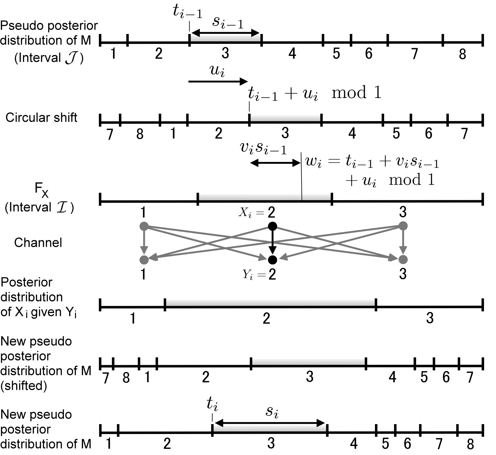
Figure 1: Illustration of the new feedback scheme for a DMC with input and output alphabet $\{1,2,3\}$. The message $M=3$ is transmitted. At time $i$, symbol $X_{i}=2$ is transmitted and symbol $Y_{i}=2$ is received.

We are now ready to formally describe our scheme. At time $i\in[1:n]$, the encoder transmits

$$X_{i}=F_{X}^{-1}(W_{i}),\quad W_{i}=w_{i}(M,Y^{i-1},U^{i},V_{i}),$$

where

$$w_{i}(m,y^{i-1},u^{i},v_{i})\! =\!v_{i}(m,y^{i-1},u^{i})\!\cdot\!s_{i-1}(m,y^{i-1},u^{i-1})$$

$$\;\;\,+t_{i-1}(m,y^{i-1},u^{i-1})+u_{i}\,\mathrm{mod}\,1,$$

$$s_{0}\left(m\right) =e^{-nR},$$

$$t_{0}\left(m\right) =\left(m-1\right)e^{-nR},$$ (2)

$$s_{i}(m,y^{i},u^{i}) =\int_{[t_{i-1}(m),t_{i-1}(m)+s_{i-1}(m)]+u_{i}\,\mathrm{mod}\,1}\!\!\!\!\!\!\!\!\!\!\!\!\!\!\!\!\!\!\!\!\!\!\!\!\!\!\!\!\!\!\!\!\!\!\!\!\!\!\!\!\!\!\!\!\!\!\!\!\!\!\!\!\!\!\!\!\!\!\!\!\!\!\!\!\!\!\!\!\!\!\!\!dF_{W|Y}(w|y_{i}),$$

$$t_{i}(m,y^{i},u^{i}) =\sum_{m^{\prime}<m}s_{i}(m^{\prime},y^{i},u^{i}),$$

where $F_{W|Y}$ is given in (1). Note that in the above integral we used the notation $[t,t+s]+u\mod 1$ to mean the set $\{x+u\mod\,1\,:\,x\in[t,t+s]\}$.

Assuming message $m$ is transmitted, the encoder selects $v_{i}(m,y^{i-1},u^{i})\in[0,1]$ using the maximal information gain rule

$$v_{i}(m,y^{i-1},u^{i})= \arg\max_{v\in[0,1]}\mathbb{E}\Bigl{[}\ln s_{i}\left(m,(y^{i-1},Y_{i}),u^{i}\right)$$

$$\;\;\;\;\;\;\Bigl{|}W_{i}=w_{i}(m,y^{i-1},u^{i},v)\Bigr{]},$$ (3)

where $Y_{i}$ is distributed according to $F_{Y|W}(y|w_{i})$. Note that this is a greedy rule that maximizes the “information gain" for each channel use.

We now provide explanations for the main ingredients of our scheme.

1) To explain the rule for selecting $X_{i}$ in (2), note that at time $i$, both the encoder and the decoder know $Y^{i-1}$. The encoder generates $X_{i}(M,Y^{i-1})$ that follows $F_{X}$ as closely as possible. For a DMC,

$$\mathbb{P}\{X_{i}=x\,|\,Y^{i-1}\!=\!y^{i-1}\}\!=\!\!\sum_{m\,:\,x_{i}(m,y^{i-1})=x}\!\!\!\!\!\!\!p_{M|Y^{i-1}}(m\,|\,y^{i-1}).$$

Therefore, the distribution of $X_{i}$ is determined by how we divide the posterior probabilities of the message among the input symbols. If $M$ is continuous, we use the same trick as in posterior matching, that is, $X_{i}=F_{X}^{-1}\circ F_{M|Y^{i-1}}(M\,|\,y^{i-1})$, and $X_{i}$ would follow $F_{X}$. Since in our setting $M$ is discrete, the posterior cdf $F_{M|Y^{i-1}}$ contains jumps, and each message $m$ is mapped to an interval instead of a single point. We use $V_{i}$ to select a point on the interval and map it by $F_{X}^{-1}$ to obtain the input symbol.

2) To explain the need for the circular shift of the intervals via $U_{i}$, note that if we map a point on the interval directly to the input symbol, the chosen symbol would depend on both the position and the length of the interval corresponding to the correct message. While the length of the interval provides information about the posterior probability of the message, the position of the interval does not contain any useful information. By applying the random circular shift $U_{i}$, the analysis of the error probability involves only the interval lengths. Suppose $m$ is sent, define $S_{i}=s_{i}(m,Y^{i},U^{i})$ to be the pseudo posterior probability of the transmitted message (the length of the interval) at time $i$ and $T_{i}=t_{i}(m,Y^{i},U^{i})$ (the position of the interval). Note that $\{S_{i}\}$ forms a Markov chain, and its transition can be specified by

$$S_{i}=\int_{[0,S_{i-1}]+\tilde{U}_{i}\,\mathrm{mod}\,1}dF_{W|Y}(w|Y_{i}),$$

where $Y_{i}\sim p_{Y|W}(\,\cdot\,|W_{i})$ is independent of $\tilde{U}^{i}$, $S^{i-1}$ and $Y^{i-1}$, and

$$W_{i} =V_{i}\cdot S_{i-1}+\tilde{U}_{i}\,\mathrm{mod}\,1,$$

$$V_{i} =\arg\max_{v\in[0,1]}\mathbb{E}\left[\ln S_{i}\,|\,W_{i}=v\cdot S_{i-1}+\tilde{U}_{i}\,\mathrm{mod}\,1\right],$$

Note that $\tilde{U}_{i}=T_{i-1}+U_{i}\sim\mathrm{U}[0,1]$ is independent of $\tilde{U}^{i-1}$, $S^{i-1}$, and $Y^{i-1}$.

As a result of the random circular shift, the analysis of error reduces to studying the real-valued Markov chain $\{S_{i}\}$. This is simpler than the analysis of posterior matching, which involves keeping track of the entire posterior distribution.

3) The reason we use the maximal information gain rule in (3) to select $V_{i}$ is that it yields a better bound on the error exponent than the simpler rule of selecting $V_{i}$ uniformly at random. With this complicated rule, however, it is very difficult to calculate the posterior probabilities. Hence, in our scheme, the interval length $s_{i}(m,y^{i},u^{i})$ is an estimate of the posterior probability assuming $V_{i}$ is selected uniformly at random. In the following we explain the method of estimating the posterior probability in detail.

Define another probability distribution $\tilde{\mathbb{P}}$ on $(M,X^{n},Y^{n},W^{n},U^{n},V^{n})$ in which $X^{n}$ is also generated according to (2) but $V^{n}$ is an i.i.d. sequence with $V_{i}\sim\mathrm{U}[0,1]$ instead of using (3). The receiver uses this distribution to estimate the posterior probability of each message, i.e.,

$$s_{i}(m,y^{i},u^{i})=\tilde{\mathbb{P}}\{M=m\,|\,Y^{i}=y^{i},\,U^{i}=u^{i}\}.$$

The expression in (2) is obtained inductively using

$$\tilde{\mathbb{P}}\{M=m\,|\,Y^{i}=y^{i},\,U^{i}=u^{i}\}$$

$$\propto\tilde{\mathbb{P}}\{M=m\,|\,Y^{i-1}=y^{i-1},\,U^{i}=u^{i}\}$$

$$\;\;\;\;\cdot\tilde{\mathbb{P}}\{Y_{i}=y_{i}\,|\,M=m,\,Y^{i-1}=y^{i-1},\,U^{i}=u^{i}\},$$

where

$$\tilde{\mathbb{P}}\{M=m\,|\,Y^{i-1}=y^{i-1},\,U^{i}=u^{i}\}$$

$$\;\cdot\tilde{\mathbb{P}}\{Y_{i}=y_{i}\,|\,M=m,\,Y^{i-1}=y^{i-1},\,U^{i}=u^{i}\}$$

$$=s_{i-1}(m)\cdot\tilde{\mathbb{P}}\{Y_{i}=y_{i}\,|\,M=m,Y^{i-1}=y^{i-1},U^{i}=u^{i}\}$$

$$=s_{i-1}(m)\cdot\int_{0}^{1}\tilde{\mathbb{P}}\{Y_{i}=y_{i}\,|\,M=m,\,Y^{i-1}=y^{i-1},$$

$$\;\;\;\;\;\;U^{i}=u^{i},\,V_{i}=v\}\,dv$$

$$=s_{i-1}(m)\cdot\int_{0}^{1}\tilde{\mathbb{P}}\{Y_{i}=y_{i}\,|\,M=m,\,Y^{i-1}=y^{i-1},$$

$$\;\;\;\;\;\;U^{i}=u^{i},W_{i}=v\!\cdot\!s_{i-1}(m)+t_{i-1}(m)+u_{i}\,\mathrm{mod}\,1\}dv$$

$$=\int_{[t_{i-1}(m),t_{i-1}(m)+s_{i-1}(m)]+u_{i}\,\mathrm{mod}\,1}\!\!\!\!\!\!\!\!\!\!\!\!\!\!\!\!\!\!\!\!\!\!\!\!\!\!\!\!\!\!\!\!\!\!\!\!\!\!\!\!\!\!\!\!\!\!\!\!\!\!\!\!\!\!\!\!\!\!\!\!\!\!\!\!\!\!\!\!\!\!\!\!\!\!\!\!\!\!\tilde{\mathbb{P}}\{Y_{i}=y_{i}\,|M=m,Y^{i-1}=y^{i-1}\!,U^{i}\!=u^{i},W_{i}=w\}dw$$

$$=\int_{[t_{i-1}(m),t_{i-1}(m)+s_{i-1}(m)]+u_{i}\,\mathrm{mod}\,1}\!\!\!\!\!\!\!\!\!\!\!\!\!\!\!\!\!\!\!\!\!\!\!\!\!\!\!\!\!\!\!\!\!\!\!\!\!\!\!\!\!\!\!\!\!\!\!\!\!\!\!\!\!\!\!\!\!\!\!\!\!\!\!\!\!\!\!\!\!\!\!\!\!p_{Y|W}(y_{i}|w)\,dw.$$

Note that we write $s_{i-1}(m)=s_{i-1}(m,y^{i-1},u^{i-1})$ and $t_{i-1}(m)=t_{i-1}(m,y^{i-1},u^{i-1})$ for simplicity. Hence,

$$\tilde{\mathbb{P}}\{M=m\,|\,Y^{i}=y^{i},\,U^{i}=u^{i}\}$$

$$=\!\frac{\int_{[t_{i-1}(m),t_{i-1}(m)+s_{i-1}(m)]+u_{i}\,\mathrm{mod}\,1}p_{Y|W}(y_{i}|w)\,dw}{\sum_{\tilde{m}=1}^{|\mathcal{M}|}\!\int_{[t_{i-1}(\tilde{m}),t_{i-1}(\tilde{m})+s_{i-1}(\tilde{m})]+u_{i}\,\mathrm{mod}\,1}\!p_{Y|W}\!(y_{i}|w)dw}$$

$$=\frac{\int_{[t_{i-1}(m),t_{i-1}(m)+s_{i-1}(m)]+u_{i}\,\mathrm{mod}\,1}p_{Y|W}(y_{i}|w)\,dw}{\int_{0}^{1}p_{Y|W}\left(y_{i}|w\right)dw}$$

$$=\int_{[t_{i-1}(m),t_{i-1}(m)+s_{i-1}(m)]+u_{i}\,\mathrm{mod}\,1}\,dF_{W|Y}(w|y_{i}).$$

The quantity $s_{i}(m,y^{i},u^{i})$ can be viewed as a pseudo posterior probability of message $m$. Note that the pseudo posterior probabilities of all the messages still sum up to one, hence we know the correct message is recovered when its pseudo posterior probability is greater than $1/2$.

From the above description, the key differences between our scheme and posterior matching are as follows:

1) We apply a random circular shift $U_{i}$ to reduce the analysis of error to studying the behavior of the Markov chain $\{S_{i}\}$.

2) The message is an integer $M\in[1:e^{nR}]$ rather than a real number $\Theta\in[0,1]$. This again simplifies the analysis.

3) Instead of using the posterior probability of the message as in posterior matching, we use the maximal information gain rule, which is crucial to the analysis of the scheme.

As a result of these differences, our scheme can achieve good error exponent over the entire rate range using a simpler error probability analysis.

III Analysis of the Probability of Error

In this section, we analyze the rate and the error exponent of our scheme for DMCs. Note that in this case, $W_{i}=w\in[0,1]$ is mapped to $X_{i}=x=F_{X}^{-1}\left(w\right)$ if $F_{X}(x-1)<w\leq F_{X}(x)$. As we discussed in the previous section, the pseudo posterior probability of the transmitted message $\left\{S_{i}\right\}$ forms a Markov chain. We obtain the bound on the error exponent by analyzing this Markov chain.

In our scheme, the decoder declares $\hat{m}=\arg\max_{m^{\prime}}s_{n}(m^{\prime},y^{n},u^{n})$. Since the pseudo posterior probabilities of all the messages sum up to one, if the pseudo posterior probability of the transmitted message $S_{n}=s_{n}(m,Y^{n},U^{n})>1/2$, we can be sure that the message is recovered correctly. Hence, the probability of error is upper bounded as

$$P_{e}^{(n)} =\mathbb{P}\left\{M\neq\arg\max_{m}s_{n}(m,Y^{n},U^{n})\right\}$$

$$\leq\mathbb{P}\left\{S_{n}\leq 1/2\right\}.$$

Remark 2: An alternative approach would be to use a threshold decoder [16], which decodes to the message with posterior probability greater than a threshold $\gamma$. However, this would introduce another error event when there is a message other than the correct one with pseudo posterior probability greater than $\gamma$. As a result, we cannot analyze the error probability by studying $S_{n}$ only. Therefore we fix the threshold at $1/2$ to simplify the analysis.

To study how the error probability decays with $n$, we consider the error exponent

$$E(R)=\limsup_{n\to\infty}-n^{-1}\ln P_{e}^{(n)}(R).$$

We define the moment generating function of the ideal increment of information (or ideal moment generating function in short) for DMC as

$$\phi\left(\rho\right) =\sum_{x}p(x)\sum_{y}p(y|x)\left(\frac{p(x|y)}{p(x)}\right)^{-\rho}$$

$$=\sum_{x}p(x)\sum_{y}p(y|x)\left(\frac{p(y|x)}{\sum_{x^{\prime}}p(x^{\prime})p(y|x^{\prime})}\right)^{-\rho}.$$

The function $\ln\phi\left(\rho\right)$ is convex, and it is not difficult to check that

$$\phi^{\prime}\left(0\right)=\left.\frac{d}{d\rho}\phi\left(\rho\right)\right|_{\rho=0}=\left.\frac{d}{d\rho}\ln\phi\left(\rho\right)\right|_{\rho=0}=-I(X;Y).$$

Similarly, we define the moment generating function of the actual increment of information at $s$ (or actual moment generating function in short) as

$$\psi_{s}\left(\rho\right)=\mathbb{E}\left[\left.S_{i}^{-\rho}/S_{i-1}^{-\rho}\right|S_{i-1}=s\right].$$

The function $\ln\psi_{s}\left(\rho\right)$ is convex. To obtain the bound on the error exponent, we also need the quantity

$$\Psi=\inf_{\tau\left(s\right)}\sup_{s\in(0,1)}\psi_{s}\left(\tau\left(s\right)\right),$$

where $\tau(s)$ is nondecreasing and the infimum is taken over all nondecreasing functions $\tau:(0,1)\to[0,\infty)$. We have $\Psi\leq 1$, since we can take $\tau\left(s\right)=0$.

We introduce the following condition on a DMC, which is sufficient for our scheme to achieve the capacity.

Definition 1.

A pair of input symbols $x_{1}\neq x_{2}$ in a DMC $p(y|x)$ is said to be redundant if $p(y|x_{1})=p(y|x_{2})$ for all $y$.

Note that if the channel has redundant input symbols, we can always use only one of these symbols and ignore the others. Therefore we can assume without loss of generality that the channel has no redundant input symbols.

We are now ready to state the main result of this paper.

Theorem 1.

For any DMC $p(y|x)$ without redundant input symbols, we have $\Psi<1$, and the maximal information gain scheme can achieve the capacity. Further, for any $R<I\left(X;Y\right)$, the error exponent is lower bound as

$$E(R) \geq\sup_{\rho>0}\left\{-\rho R-\ln\max\left(\phi\left(\rho\right),\,\Psi\right)\right\}.$$

The proof of this theorem is detailed in the following subsection.

The bound on the error exponent of our scheme becomes quite tight as the rate tends to the capacity.

Corollary 1.

The error exponent $E(R)$ satisfies

$$E(R)=\frac{\left(I\left(X;Y\right)-R\right)^{2}}{2\mathrm{Var}[\ln(p(Y|X)/p(Y))]}-O\left(\left(I\left(X;Y\right)-R\right)^{3}\right)$$

as $R$ tends to $I\left(X;Y\right)$.

The quantity $\mathrm{Var}[\ln(p(Y|X)/p(Y))]$ is known as the channel dispersion [17, 18]. Note that this is the same limit as for the sphere packing bound. Hence the error exponent of our scheme tends to the sphere packing bound when the rate tends to the capacity. The proof of this corollary is given in Appendix A.

To illustrate the above results, consider the following.

Example (Binary Symmetric Channel):

Consider a binary symmetric channel with crossover probability $p$. It is well known that the capacity of this channel is achieved with $X\sim\mathrm{Bern}(1/2)$. The maximal information gain rule always selects the input symbol whose probability interval has the larger overlapping area with the message interval. The actual moment generating function is $\psi_{s}(\rho)=p\alpha+q\beta$, where $q=1-p$, and

$$\alpha =\!\begin{cases}(2p)^{-\rho}\bigg{(}1-2s+\frac{4sp}{(\rho-1)(q-p)}\bigg{)}+\frac{2s}{\rho-1}&s\leq\frac{1}{2},\\[6.0pt] (2s-1)\big{(}2q-\frac{q-p}{s}\big{)}^{-\rho}-\frac{2s(1-(2q-(q-p)/s)^{1-\rho})}{(\rho-1)(q-p)}\!\!&s>\frac{1}{2},\end{cases}$$

$$\beta =\!\begin{cases}(2q)^{-\rho}\bigg{(}1-2s-\frac{4sq}{(\rho-1)(q-p)}\bigg{)}+\frac{2s}{\rho-1}&s\leq\frac{1}{2},\\[6.0pt] (2s-1)\big{(}2p+\frac{q-p}{s}\big{)}^{-\rho}+\frac{2s(1-(2p-(q-p)/s)^{1-\rho})}{(\rho-1)(q-p)}\!\!&s>\frac{1}{2}.\end{cases}$$

The value of $\Psi$ can be found approximately using dynamic programming. For example, for $\mathrm{BSC}(0.1)$, $\Psi\approx 0.8948$.

Figure 2 compares the bound on the error exponent for our scheme to the following.

1) The sphere packing exponent $\max_{Q}\max_{\rho>0}E_{0}\left(\rho,Q\right)-\rho R$, where

$$E_{0}\left(\rho,Q\right)=-\ln\sum_{y}\left(\sum_{x}Q\left(x\right)p\left(y|x\right)^{1/\left(1+\rho\right)}\right)^{1+\rho}.$$

2) The random coding exponent $\max_{Q}\max_{\rho\in(0,1]}E_{0}\left(\rho,Q\right)-\rho R$, which is a lower bound without feedback.

3) The dependence-testing (DT) bound [16], which is the error exponent for random coding without feedback when a threshold decoder is used.

Note that our error exponent approaches the sphere packing exponent when $R$ is close to the capacity. Also our exponent almost coincides with the DT bound, with noticeable difference only when the rate is close to zero.

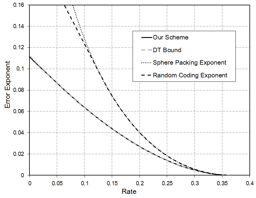
Figure 2: Comparisons of the bound on the error error exponent for a $\mathrm{BSC}(0.1)$.

III-A Proof of Theorem 1

We first outline the main ideas of the proof of the theorem. As we discussed, to analyze the error probability of our scheme, it suffices to study how $S_{i}$ increases from $S_{0}=e^{-nR}$ to $S_{n}>1/2$. We divide the analysis of the scheme by the stage of transmissions into: the starting phase, where $S_{i}$ is small, the transition phase, where $S_{i}$ is not close to $0$ or $1$, and the ending phase, where $S_{i}$ is close to $1$. We outline the proof for each phase.

The starting phase refers to the transmission period in which $S_{i}\leq S_{\mathrm{start}}$, where $S_{\mathrm{start}}$ is a constant that depends on the channel. During this phase, the length of the message interval $[T_{i-1}+U_{i},T_{i-1}+S_{i-1}+U_{i}]\mod 1$ is close to $0$ and is very likely to overlap with the probability interval $[F_{X}\left(x-1\right),F_{X}\left(x\right)]$ for only a single input symbol $x$ as illustrated in Figure 3. In this case, the maximal information gain rule selects $x$ and the probability of $X_{i}$ would be close to $p(x)$. The following lemma shows that in this regime the actual moment generating function is close to the ideal one.

Lemma 1 (starting phase MGF).

For any DMC $p(y|x)$ with input pmf $p(x)$, let $S_{\mathrm{start}}=\min_{x\,:\,p(x)>0}p\left(x\right)$, then there exists $\omega\geq 1$ such that

$$\left(1-\frac{s}{S_{\mathrm{start}}}\right)\phi\left(\rho\right)+\frac{s}{S_{\mathrm{start}}}\omega^{-\rho}\leq\psi_{s}\left(\rho\right)$$

$$\qquad\qquad\qquad\qquad\qquad\leq\left(1-\frac{s}{S_{\mathrm{start}}}\right)\phi\left(\rho\right)+\frac{s}{S_{\mathrm{start}}}\omega^{\rho}$$

for $s\leq S_{\mathrm{start}}$ and $\rho\geq 0$.

The proof of the lemma is given in Appendix B.

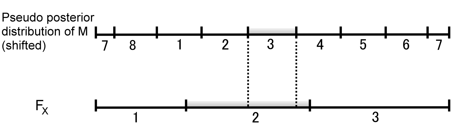
Figure 3: Illustration of the shifted pseudo posterior distribution during the starting phase (assuming $M=3$ is sent).

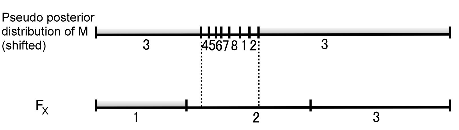
Figure 4: Illustration of the shifted pseudo posterior distribution during the ending phase (assuming $M=3$ is transmitted).

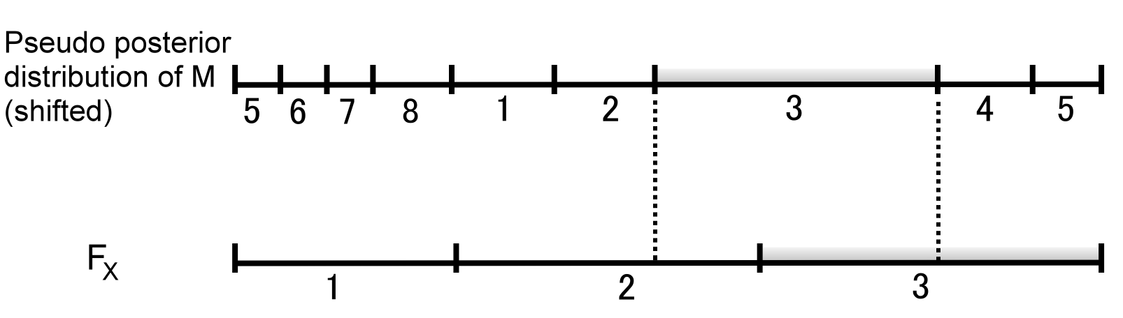
Figure 5: Illustration of the shifted pseudo posterior distribution during the transition phase (assuming $M=3$ is sent).

The ending phase refers to the transmission period in which $S_{i}\geq S_{\mathrm{end}}$, where $S_{\mathrm{end}}$ is a constant that depends on the channel. During the ending phase, the length of the message interval $[T_{i-1}+U_{i},T_{i-1}+S_{i-1}+U_{i}]\mod 1$ is close to one. Hence, the maximal information gain rule is free to select any input symbol. However, the complement of the message interval is likely to overlap with only one symbol probability interval $[F_{X}\left(\bar{x}-1\right),F_{X}\left(\bar{x}\right)]$ as illustrated in Figure 4. In this case, the maximal information gain rule selects the input symbol $x$, which is the “opposite" of $\bar{x}$ in the sense that the posterior probability of $X_{i}=\bar{x}$ is minimized when $X_{i}=x$ is transmitted. This would maximize the posterior probability of the message. We can bound the actual moment generating function during this phase as follows.

Lemma 2 (ending phase MGF).

For any DMC $p(y|x)$, there exists $0<S_{\mathrm{end}}<1$, $\gamma>0$ and $\Psi_{\mathrm{end}}<1$ such that when $s\geq S_{\mathrm{end}}$,

$$\psi_{s}\left(\gamma\left(1-s\right)^{-1}\right)\leq\Psi_{\mathrm{end}}.$$

The proof of the lemma is given in Appendix C.

The transition phase refers to the transmission period in which $S_{\mathrm{start}}<S_{i}<S_{\mathrm{end}}$ as illustrated in Figure 5. For the error exponent in Theorem 1 to be nonzero, we need $\Psi<1$, therefore we need to find a nondecreasing function $\tau:(0,1)\to[0,\infty)$ such that $\psi_{s}\left(\tau\left(s\right)\right)$ is bounded above and away from $1$. From the plot in Figure 6, we can see that $\psi_{s}\left(\rho\right)$ is well-behaved in the starting and ending phases, but not in the transition phase. Nevertheless, it is possible to construct $\tau$ satisfying the requirement, as shown in the following lemma.

Lemma 3.

For a DMC $p(y|x)$ without redundant input symbols, we have $\Psi<1$.

The proof of the lemma is given in Appendix D.

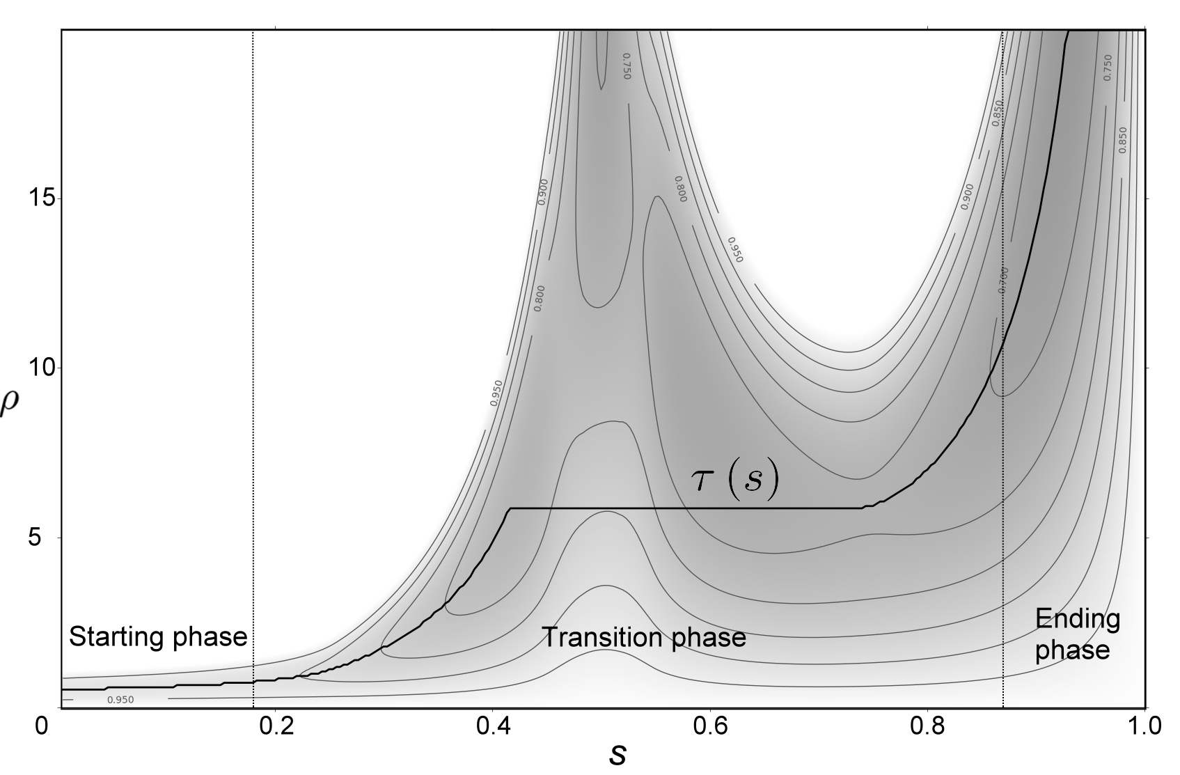
Figure 6: Contour plot of $\psi_{s}\left(\rho\right)$ for an example channel. Darker color indicates smaller $\psi_{s}\left(\rho\right)$. The minimizing function $\tau\left(s\right)$ is also plotted.

To show that our scheme achieves the capacity, recall that $S_{i}$ should increase from $S_{0}=e^{-nR}$ to $S_{n}>1/2$, or equivalently, $-\ln S_{i}$ should decrease from $-\ln S_{0}=nR$ to $-\ln S_{n}<\ln 2$. When $n$ is large, $S_{0}$ is close to zero; hence the time spent in the starting phase would dominate. Since the actual moment generating function is close to the ideal one during this phase, we expect the decrease in $-\ln S_{i}$ for each time step to be close to $-\phi^{\prime}\left(0\right)=I(X;Y)$. Therefore as long as $R<I(X;Y)$, $-\ln S_{i}$ would decrease from $nR$ to a value smaller than $\ln 2$ in $n$ time steps. However, we still need to show that the transition and the ending phase would not affect the performance of the code. As we will see in the proof of the theorem, the fact that $\Psi<1$ is sufficient for this purpose.

We now discuss the details of the proof of Theorem 1.

Let $\rho^{*}$ be the maximizer of $-\rho R-\ln\max\left\{\phi\left(\rho\right),\,\Psi\right\}$, and define

$$\tau_{2}\left(s\right)=\begin{cases}\rho^{*}-\epsilon&\text{ when }s<\xi\\ \tau\left(s\right)&\text{ when }s\geq\xi,\end{cases}$$

and

$$g\left(s\right)=\exp\left(-\int_{\xi}^{s}\tau_{2}\left(r\right)r^{-1}\,dr\right),$$

where $\epsilon$ and $\xi$ are suitable constants.

We now use Lemma 1 to 3 to prove the theorem. The main idea is to design a function $g(s)$ and apply the Markov inequality to $g(S_{n})$. Note that $\frac{d}{d\rho}\ln\phi\left(\rho\right)$ is continuous at $\rho=0$ and $\left.\frac{d}{d\rho}\ln\phi\left(\rho\right)\right|_{\rho=0}=-I(X;Y)$, therefore, $-R\rho-\ln\max\left\{\phi\left(\rho\right),\,\psi\right\}$ is positive when $\rho$ is small. If the proposed bound on the error exponent holds, then $E\left(R\right)>0$ for any $R<I(X;Y)$, and thus capacity can be achieved.

Let $\rho^{*}$ be the maximizer of $-\rho R-\ln\max\left(\phi\left(\rho\right),\,\Psi\right)$. Since $\phi\left(\rho\right)$ is continuous, we may assume $\phi\left(\rho^{*}\right)\geq\Psi$. Let $\epsilon>0$ and $\tau^{*}\left(s\right)>0$ be a nondecreasing function such that

$$\Psi e^{\epsilon}\geq\psi_{s}\left(\tau^{*}\left(s\right)\right)$$

for all $s\in(0,1)$.

By Lemma 1, there exists $\xi_{2}$ such that when $s\leq\xi_{2}$, we have $\psi_{s}\left(\rho\right)\leq\phi\left(\rho\right)e^{\epsilon}$ for $\rho\leq\rho^{*}-4\epsilon/R$. Again by Lemma 1, there exists $\xi\leq\xi_{2}$ such that when $s\leq\xi$, we have $\phi\left(\rho\right)\leq\psi_{s}\left(\rho\right)e^{\epsilon}$ for $\rho\leq\tau^{*}\left(\xi_{2}\right)$. Define

$$\tau\left(s\right)=\begin{cases}\rho^{*}-4\epsilon/R&\text{ when }s<\xi\\ \tau^{*}\left(s\right)&\text{ when }s\geq\xi.\end{cases}$$

Note that

$$\ln\phi\left(\tau^{*}\left(\xi\right)\right) \leq\ln\psi_{\xi}\left(\tau^{*}\left(\xi\right)\right)+\epsilon$$

$$\leq\ln\Psi+2\epsilon$$

$$\leq\ln\phi\left(\rho^{*}\right)+2\epsilon$$

$$<\ln\phi\left(\rho^{*}-4\epsilon/R\right).$$

This implies that $\tau^{*}\left(\xi\right)\geq\rho^{*}-4\epsilon/R$ by the convexity of $\phi\left(\rho\right)$. Hence $\tau\left(s\right)$ is nondecreasing. Define

$$g\left(s\right)=\exp\left(-\int_{\xi}^{s}\tau\left(r\right)r^{-1}\,dr\right).$$

We then consider the quantity $\mathbb{E}\left[g\left(S_{i}\right)\right]$. Note that $g\left(s\right)$ is nonincreasing, hence

$$\mathbb{E}\left[\left.g\left(S_{i}\right)/g\left(S_{i-1}\right)\right|S_{i-1}=s\right]$$

$$=\mathbb{E}\left[\left.\exp\left(-\int_{s}^{S_{i}}\tau\left(r\right)r^{-1}\,dr\right)\right|S_{i-1}=s\right]$$

$$\leq\mathbb{E}\left[\left.\exp\left(-\int_{s}^{S_{i}}\tau\left(s\right)r^{-1}\,dr\right)\right|S_{i-1}=s\right]$$

$$=\mathbb{E}\left[\left.S_{i}^{-\tau\left(s\right)}/s^{-\tau\left(s\right)}\right|S_{i-1}=s\right]$$

$$\leq\max\left(\phi\left(\rho^{*}-4\epsilon/R\right)e^{\epsilon},\,\Psi e^{\epsilon}\right)$$

$$=\phi\left(\rho^{*}-4\epsilon/R\right)e^{\epsilon}.$$

Decoding succeeds if $S_{n}\geq 2/3>1/2$. Since $g\left(S_{0}\right)=e^{\left(\rho^{*}-2\epsilon/R\right)nR}/\xi^{-\left(\rho^{*}-2\epsilon/R\right)}$, we have

$$\mathbb{P}\left\{S_{n}<2/3\right\} \leq\mathbb{E}\left[g\left(S_{n}\right)\right]/g\left(2/3\right)$$

$$\leq\frac{e^{\left(\rho^{*}-4\epsilon/R\right)nR}}{\xi^{-\left(\rho^{*}-4\epsilon/R\right)}}\cdot\frac{\left(\phi\left(\rho^{*}-4\epsilon/R\right)e^{\epsilon}\right)^{n}}{g\left(2/3\right)}$$

$$=\frac{1}{\xi^{-\left(\rho^{*}-4\epsilon/R\right)}g\left(2/3\right)}$$

$$\;\;\;\cdot\exp\left(-n\!\cdot\!\left(-\rho^{*}R\!+\!\epsilon\!-\!\ln\left(\phi\left(\rho^{*}\!-\!4\epsilon/R\right)\right)\right)\right).$$

The proof of the theorem is completed by letting $\epsilon\to 0$.

IV Coding Complexity

In this section, we briefly discuss the implementation of our coding algorithm and show that its computational complexity for DMCs is $O\left(n\log n\right)$ and its memory complexity is $O\left(n\right)$.

Although there are $e^{nR}$ possible messages, most of them share the same pseudo posterior probability, so instead of storing the pseudo posterior probabilities of the messages separately, we store intervals of message points with the same pseudo posterior probability. We use one binary search tree to keep track of boundary points of these intervals, and another self balancing binary search tree to keep track of the cumulative pseudo posterior probabilities up to their boundary points. The encoder and the decoder both keep and update a copy of each tree (which holds the same content due to feedback).

We implemented the self balancing tree by a splay tree [19]. For $n$ transmissions, the number of nodes in the tree is at most $n\left|\mathcal{X}\right|$, and therefore the queries and the updates can be done in $O\left(n\left|\mathcal{X}\right|\log\left(n\left|\mathcal{X}\right|\right)\right)=O\left(n\log n\right)$, and the memory complexity is $O\left(n\right)$. Detailed description of this implementation can be found in [15].

To corroborate our analysis, we performed simulations of our algorithm assuming a $\mathrm{BSC}(0.1)$ and rate $R=0.98C$ with $n$ from $2000$ to $100,000$. For each $n$, $150$ independent trials are run to obtain an average running time and an estimate of the error probability. Figure 7 shows that the average running time is close to linear.

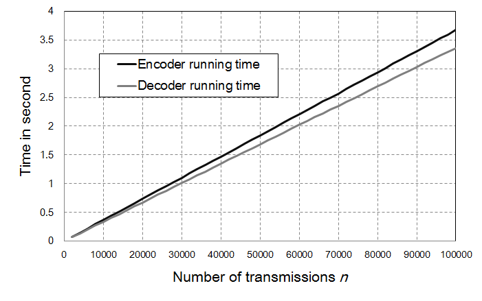
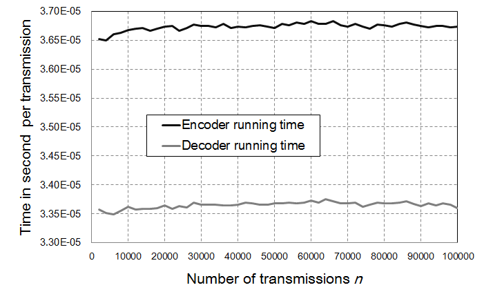
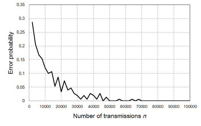
Figure 7: Top: Running time of our coding algorithm for $\mathrm{BSC}(0.1)$ versus the number of channel uses $n$. Middle: Running time divided by $n$. Bottom: Empirical error probability (the portion of trials where the decoded message does not match the transmitted one).

V Conclusion

We proposed a new low coding complexity feedback coding scheme which achieves the capacity of all DMCs. Our scheme is much easier to analyze than posterior matching, making it possible to establish a lower bound on the error exponent that is close to the sphere packing bound at high rate. It would be interesting to explore if our scheme can be modified so that the error exponent exactly coincides with the sphere packing bound when the rate is above a certain threshold. Another possible extension is to investigate whether our scheme achieves the channel dispersion given in [18]. Although variable-length coding with feedback can achieve zero dispersion [20], this may not be achievable using our scheme since it is fixed-length.

VI Acknowledgments

The authors are indebted to Young-Han Kim, Chandra Nair, Tsachy Weissman, and the anonymous reviewers for invaluable comments that have greatly improved the exposition of the results in this paper.

Appendix A Proof of Corollary 1

Recall that the error exponent in Theorem 1 is

$$E(R) \geq\sup_{\rho>0}\left\{-\rho R-\ln\max\left(\phi\left(\rho\right),\,\Psi\right)\right\}.$$

Consider the Taylor expansion of $\ln\phi\left(\rho\right)$ at $\rho=0$,

$$\ln\phi\left(\rho\right)$$

$$=\ln\sum_{y}\left(\sum_{x}p(x)p(y|x)^{1-\rho}\right)\left(\sum_{x}p(x)p(y|x)\right)^{\rho}$$

$$=\rho\cdot-I\left(X;Y\right)+\frac{\rho^{2}}{2}\cdot\sigma^{2}+O\left(\rho^{3}\right),$$

where

$$\sigma^{2}=\mathrm{Var}[\ln(p(Y|X)/p(Y))]$$

$$\;\;=\mathbb{E}\left[\ln(p(Y|X)/p(Y))^{2}\right]-\mathbb{E}\left[\ln(p(Y|X)/p(Y))\right]^{2}$$

$$\;\;=\!\sum_{x}\!\sum_{y}p(x)p(y|x)\!\left(\ln\frac{p(y|x)}{\sum_{x^{\prime}}p(x^{\prime})p(y|x^{\prime})}\right)^{2}\!\!\!-\!I\left(X;\!Y\right)^{2}\!.$$

Take $\rho=\sigma^{-2}\left(I\left(X;Y\right)-R\right)$. As $R\to I(X;Y)$, we have $\rho\to 0$, and therefore $\phi\left(\rho\right)\to 1$ will be larger than $\Psi$, and

$$E(R) \geq-\rho R-\ln\phi\left(\rho\right)$$

$$=\rho\left(I\left(X;Y\right)-R\right)-\frac{\rho^{2}}{2}\cdot\sigma^{2}-O\left(\rho^{3}\right)$$

$$=\frac{1}{2}\sigma^{-2}\left(I\left(X;Y\right)\!-\!R\right)^{2}\!-O\left(\left(I\left(X;Y\right)-R\right)^{3}\right).$$

This completes the proof of the corollary.

Appendix B Proof of Lemma 1 (Starting Phase MGF)

Assume $S_{0}=s\leq S_{\mathrm{start}}$, then

$$S_{1} =\int_{[0,s]+U_{1}\,\mathrm{mod}\,1}dF_{W|Y}\left(w|Y_{1}\right)$$

$$=\int_{[-s/2,s/2]+U^{\prime}_{1}\,\mathrm{mod}\,1}dF_{W|Y}\left(w|Y_{1}\right),$$

where $U^{\prime}_{1}=U_{1}+\left(s/2\right)\,\mathrm{mod}\,1$. Note that $F_{X}^{-1}(w)=x$ if $F_{X}(x-1)<w\leq F_{X}(x)$. Let $\alpha=s/\min_{x}p\left(x\right)$, and let $A$ be the event that

$$\left(1-\frac{\alpha}{2}\right)F_{X}(x-1)+\frac{\alpha}{2}F_{X}(x)<U^{\prime}_{1}$$

$$\;\;\;\;\;\;\;\;\;\;\;\;\;\;\;\;\;\;\;\;\;\;\;\;\;\;\;\;\leq\frac{\alpha}{2}F_{X}(x-1)+\left(1-\frac{\alpha}{2}\right)F_{X}(x)$$

for some $x$. Then $\mathbb{P}\left\{A\right\}=1-\alpha$. Note that $A$ is independent of $F_{X}^{-1}\left(U^{\prime}_{1}\right)$ (the input symbol that $U^{\prime}_{1}$ is mapped to). Conditioned on $A$, the intervals $[-s/2,s/2]+U^{\prime}_{1}\,\mathrm{mod}\,1$ does not cross the boundary points $F_{X}(x)$, and we have $S_{1}=S_{0}+\ln p_{X|Y}\left(F_{X}^{-1}\left(U^{\prime}_{1}\right)|Y_{1}\right)/p_{X}\left(F_{X}^{-1}\left(U^{\prime}_{1}\right)\right)$.

We now show that $S_{0}/S_{1}$ is almost surely bounded by a constant independent of $S_{0}=s$. Note that

$$S_{0}/S_{1}\geq\min_{x,y:p\left(x|y\right)>0}\frac{p\left(x\right)}{p\left(x|y\right)}\overset{def}{=}\omega_{\mathrm{lower}}$$

almost surely. Next we establish an upper bound. If $p\left(x|y\right)>0$ for any $x,y$, then

$$S_{0}/S_{1}\leq\max_{x,y}\frac{p\left(x\right)}{p\left(x|y\right)}.$$

Note that when $S_{0}\leq\min_{x}p\left(x\right)$, the interval $[0,s)+U_{1}\,\mathrm{mod}\,1$ intersects at most one boundary point $F_{X}(x)$. Assume $F_{X}(i)\in\left([0,s)+U_{1}\,\mathrm{mod}\,1\right)$, and let $r=s^{-1}\left(F_{X}(i)-(U_{1}\,\mathrm{mod}\,1)\right)$ be the portion of the interval lying in the $X=i$ region, then the maximal information gain scheme would select $X$ among $x\in\{i,i+1\}$ that gives a larger

$$\mathbb{E}\left[\left.\ln\left(rp\left(i|Y\right)+\left(1-r\right)p\left(i+1|Y\right)\right)\right|X=x\right]\overset{def}{=}b_{x}\left(r\right).$$

If we have $p_{Y|X}\left(y|i+1\right)>0$ for any $y$ with $p_{Y|X}\left(y|i\right)>0$, then $S_{0}/S_{1}\leq\max_{x,y:p(x|y)>0}p(x)/p(x|y)$ holds when $X=i$. Otherwise there exists a $y$ such that $p_{Y|X}\left(y|i\right)>0$, $p_{Y|X}\left(y|i+1\right)=0$, then $b_{i}\left(r\right)\to-\infty$ when $r\to 0$. By continuity, assume $b_{i+1}\left(r\right)>b_{i}\left(r\right)$ for $r<r_{i,i+1}$, then when $X=i$ we have $r\geq r_{i,i+1}$, and

$$S_{0}/S_{1}\leq r_{i,i+1}^{-1}\max_{x,y:p\left(x|y\right)>0}\frac{p\left(x\right)}{p\left(x|y\right)}$$

almost surely. Define $r_{i+1,i}$ similarly. Therefore $S_{0}/S_{1}\leq\omega_{\mathrm{upper}}\overset{def}{=}\big{(}\max_{i,j}r_{i,j}^{-1}\big{)}\big{(}\max_{x,y:p(x|y)>0}p(x)/p(x|y)\big{)}$, and

$$\left(1-\alpha\right)\phi\left(\rho\right)+\alpha\omega_{\mathrm{lower}}^{\rho}\leq\mathbb{E}\left[\left.S_{1}^{-\rho}/S_{0}^{-\rho}\right|S_{0}=s\right]$$

$$\;\;\;\;\;\;\;\;\;\;\;\;\;\;\;\;\;\;\;\;\;\;\;\;\;\;\;\;\;\;\;\;\;\;\;\;\;\;\;\;\;\;\;\;\;\;\leq\left(1-\alpha\right)\phi\left(\rho\right)+\alpha\omega_{\mathrm{upper}}^{\rho}.$$

The proof of Lemma 1 is completed by letting $\omega=\max\left\{\omega_{\mathrm{upper}},\omega_{\mathrm{lower}}^{-1}\right\}$.

Appendix C Proof of Lemma 2 (Ending Phase MGF)

Assume $S_{0}=s\geq 1-\xi$. Note that the interval of the message $[0,s]+U_{1}\,\mathrm{mod}\,1$ overlaps all the intervals corresponding to the input symbols. Therefore the encoder can choose among all symbols the one that minimizes the expected value of $-\ln S_{1}$.

$$S_{1} =\int_{[0,s]+U_{1}\,\mathrm{mod}\,1}dF_{W|Y}\left(w|Y_{1}\right)$$

$$=1-\int_{[-\left(1-s\right)/2,\left(1-s\right)/2]+U^{\prime}_{1}\,\mathrm{mod}\,1}dF_{W|Y}\left(w|Y_{1}\right),$$

where $U^{\prime}_{1}=U{}_{1}+\left(\left(1+s\right)/2\right)\,\mathrm{mod}\,1$. Note that $F_{X}^{-1}(w)=x$ if $F_{X}(x-1)<w\leq F_{X}(x)$. Let $\alpha=\left(1-s\right)/\min_{x}p\left(x\right)$, and let $A$ be the event that

$$\left(1-\frac{\alpha}{2}\right)F_{X}(x-1)+\frac{\alpha}{2}F_{X}(x)<U^{\prime}_{1}$$

$$\;\;\;\;\leq\frac{\alpha}{2}F_{X}(x-1)+\left(1-\frac{\alpha}{2}\right)F_{X}(x)$$

for some $k$. Then $\mathbb{P}\left\{A\right\}=1-\alpha$. Note that $A$ is independent of $F_{X}^{-1}\left(U^{\prime}_{1}\right)$ (the input symbol that $U^{\prime}_{1}$ is mapped to).

Conditioned on $A$ and $U^{\prime}_{1}=u^{\prime}_{1}$, the intervals $[-\left(1-s\right)/2,\left(1-s\right)/2]+U^{\prime}_{1}\,\mathrm{mod}\,1$ does not cross the boundary points $F_{X}(x)$. Assume the interval maps to $x_{1}=F_{X}^{-1}\left(u^{\prime}_{1}\right)$. Define the opposite symbol $\mathrm{opp}\left(x_{1}\right)$ as the symbol $\bar{x}_{1}$ that minimizes

$$\mathbb{E}\left[\left.p_{X|Y}\left(x_{1}|Y\right)\right|X=\bar{x}_{1}\right].$$

In case of a tie, choose the symbol that minimizes $\mathbb{E}\left[\left.\left(p_{X|Y}\left(x_{1}|Y\right)\right)^{2}\right|X=\bar{x}_{1}\right]$, and so on. Since

$$\mathbb{E}\left[\left.-\ln S_{1}\right|U^{\prime}_{1}=u^{\prime}_{1},X=x\right]$$

$$=\mathbb{E}\Bigl{[}-\ln\Bigl{(}1-\int_{[-\frac{1-s}{2},\frac{1-s}{2})+u^{\prime}_{1}\,\mathrm{mod}\,1}\!\!\!\!\!\!\!\!\!\!\!\!\!\!\!\!\!\!\!\!\!\!\!\!\!\!\!\!dF_{W|Y}\left(w|Y\right)\Bigr{)}\Bigr{|}X=x\Bigr{]}$$

$$=\mathbb{E}\Bigl{[}-\ln\Bigl{(}1-\frac{1-s}{p_{X}\left(x_{1}\right)}p_{X|Y}\left(x_{1}|Y\right)\Bigr{)}\Bigr{|}X=x\Bigr{]}$$

$$=\sum_{k=1}^{K}k^{-1}\Bigl{(}\frac{1-s}{p_{X}\left(x_{1}\right)}\Bigr{)}^{k}\mathbb{E}\left[\left.\left(p_{X|Y}\left(x_{1}|Y\right)\right)^{k}\right|X=x\right]$$

$$\;\;\;\;+O\Bigl{(}\left(1-s\right)^{K+1}\Bigr{)}$$

by the Taylor series expansion, we can find $S_{\mathrm{end}}$ such that the maximal information gain scheme chooses $\mathrm{opp}\left(x_{1}\right)=\mathrm{opp}\left(F_{X}^{-1}\left(u^{\prime}_{1}\right)\right)$ whenever $s\geq S_{\mathrm{end}}$ and $u^{\prime}_{1}$ satisfies the conditions of the event $A$.

Note that $p_{X}\left(x_{1}\right)$ is the weighted mean of $\mathbb{E}\left[\left.p_{X|Y}\left(x_{1}|Y\right)\right|X=\bar{x}_{1}\right]$ over $\bar{x}_{1}$, and those values are not all equal (or else the capacity of the channel is zero), we have, for any $x_{1}$,

$$\mathbb{E}\left[\left.p_{X|Y}\left(x_{1}|Y\right)\right|X=\mathrm{opp}\left(x_{1}\right)\right]\leq\left(1-\eta\right)p_{X}\left(x_{1}\right)$$

for a constant $\eta>0$ which does not depend on $x_{1}$.

Assume $S_{\mathrm{end}}$ is close enough to $1$ such that $s^{-\left(1-s\right)^{-1}}\geq e^{1-\eta/4}$ for $s\geq S_{\mathrm{end}}$.

$$\mathbb{E}\left[\left.S_{1}^{-\gamma\left(1-s\right)^{-1}}\right|A,S_{0}=s\right]$$

$$=\mathbb{E}\biggl{[}\biggl{(}1-\frac{p_{X|Y}\left(F_{X}^{-1}\left(U^{\prime}_{1}\right)|Y\right)}{p_{X}\left(F_{X}^{-1}\left(U^{\prime}_{1}\right)\right)}\left(1-s\right)\biggr{)}^{-\gamma\left(1-s\right)^{-1}}$$

$$\;\;\;\;\;\;\;\;\;\;\;\;\biggl{|}X=\mathrm{opp}\left(F_{X}^{-1}\left(U^{\prime}_{1}\right)\right),S_{0}=s\biggr{]}$$

$$\leq\max_{x\in\mathcal{X}}\mathbb{E}\biggl{[}\Big{(}1-\frac{p_{X|Y}\left(x|Y\right)}{p_{X}\left(x\right)}\left(1-s\right)\Big{)}^{-\gamma\left(1-s\right)^{-1}}$$

$$\;\;\;\;\;\;\;\;\;\;\;\;\biggl{|}X=\mathrm{opp}\left(x\right),S_{0}=s\biggr{]}$$

$$\leq\max_{x\in\mathcal{X}}\mathbb{E}\biggl{[}\exp\Bigl{(}\gamma\Bigl{(}\frac{p_{X|Y}\left(x|Y\right)}{p_{X}\left(x\right)}+\frac{\eta}{8}\Bigr{)}\Bigr{)}$$

$$\;\;\;\;\;\;\;\;\;\;\;\;\biggl{|}X=\mathrm{opp}\left(x\right),S_{0}=s\biggr{]}$$

$$\leq\max_{x\in\mathcal{X}}\exp\biggl{(}\mathbb{E}\biggl{[}\gamma\Bigl{(}\frac{p_{X|Y}\left(x|Y\right)}{p_{X}\left(x\right)}+\frac{\eta}{4}\Bigr{)}$$

$$\;\;\;\;\;\;\;\;\;\;\;\;\bigg{|}X=\mathrm{opp}\left(x\right),S_{0}=s\biggr{]}\biggr{)}$$

$$\leq\exp\left(\gamma\left(\left(1-\eta\right)+\eta/4\right)\right)$$

$$=e^{\gamma\left(1-\eta/4\right)}e^{-\eta\gamma/2}$$

for $S_{\mathrm{end}}$ is close enough to $1$ and $\gamma=\gamma\left(\eta,S_{\mathrm{end}}\right)>0$ small enough (depend only on the channel, $\eta$ and $S_{\mathrm{end}}$). The third line from the bottom can be shown by differentiating the expressions with respect to $\gamma$. We have

$$\mathbb{E}\left[\left.S_{1}^{-\gamma\left(1-s\right)^{-1}}/S_{0}^{-\gamma\left(1-s\right)^{-1}}\right|A,S_{0}=s\right]$$

$$\leq e^{-\gamma\left(1-\eta/4\right)}\mathbb{E}\left[\left.S_{1}^{-\gamma\left(1-s\right)^{-1}}\right|A,S_{0}=s\right]$$

$$\leq e^{-\eta\gamma/2}.$$

Define $\omega=\max_{x,y:p\left(x\right)>0}\frac{p\left(x|y\right)}{p\left(x\right)}$, then

$$S_{1}^{-\gamma\left(1-s\right)^{-1}}/S_{0}^{-\gamma\left(1-s\right)^{-1}} \leq\left(1-\omega\left(1-s\right)\right)^{-\gamma\left(1-s\right)^{-1}}s^{\gamma\left(1-s\right)^{-1}}$$

$$\leq e^{\gamma\left(1+\omega-\eta/4\right)}.$$

Hence,

$$\psi_{s}\left(\gamma\left(1-s\right)^{-1}\right) =\left(1-\alpha\right)e^{-\eta\gamma/2}+\alpha e^{\gamma\left(1+\omega-\eta/4\right)}$$

$$\leq e^{-\eta\gamma/2}+\frac{1-s}{\min_{x_{k}}p\left(x_{k}\right)}e^{\gamma\left(1+\omega-\eta/4\right)}$$

$$\leq e^{-\eta\gamma/4}$$

for $1-s$ small enough. This completes the proof of Lemma 2.

Appendix D Proof of Lemma 3

By Lemma 2, when $S_{i}\geq S_{\mathrm{end}}$, the actual moment generating function can be bounded. It is left to bound the actual MGF for $S_{i}<S_{\mathrm{end}}$. We first prove that $\psi_{s}^{\prime}\left(0\right)$ for $s\leq S_{\mathrm{end}}$ can be bounded above and away from $0$.

Since the maximal information gain rule (3) minimizes the expectation of $-\ln S_{i}$, it has a smaller $\mathbb{E}\left[-\ln S_{i}\right|S_{i-1}=s]$ than any other rule of selecting $V_{i}$. In particular, if we generate $V_{i}$ according to $\mathrm{U}[0,1]$, the expectation would be $\tilde{\mathbb{E}}[-\ln S_{i}|S_{i-1}=s]$, where $\tilde{\mathbb{E}}$ denotes the expectation under the probability measure $\tilde{\mathbb{P}}$. Therefore,

$$\mathbb{E}[-\ln S_{i}|S_{i-1}=s]$$

$$\leq\tilde{\mathbb{E}}[-\ln S_{i}|S_{i-1}=s]$$

$$=\tilde{\mathbb{E}}\biggl{[}-\ln\int_{[T_{i-1},T_{i-1}+s]+U_{i}\,\mathrm{mod}\,1}f_{W|Y}(w|Y_{i})\,dw\biggr{]}$$

$$=\tilde{\mathbb{E}}\biggl{[}-\ln\int_{[T_{i-1},T_{i-1}+s]+U_{i}\,\mathrm{mod}\,1}\frac{f_{Y|W}(Y_{i}|w)}{f_{Y}(Y_{i})}\,dw\biggr{]}$$

$$=\tilde{\mathbb{E}}\biggl{[}-\ln\int_{[0,s]+U_{i}\,\mathrm{mod}\,1}\frac{f_{Y|W}(Y_{i}|w)}{f_{Y}(Y_{i})}\,dw\,\Big{|}\,T_{i-1}=0\biggr{]}$$

$$=\int_{0}^{1}\!\int_{[0,s]+u\,\mathrm{mod}\,1}\int\!\biggl{(}\!-\!\ln\!\int_{[0,s]+u\,\mathrm{mod}\,1}\!\!\!\frac{f_{Y|W}(y|w)}{f_{Y}(y)}\,dw\!\biggr{)}$$

$$\;\;\;\cdot f_{Y|W}\left(y|w_{0}\right)dy\cdot s^{-1}\,dw_{0}\cdot du$$

$$=-\ln s+\int_{0}^{1}\int\biggl{(}\int_{[0,s]+u\,\mathrm{mod}\,1}f_{Y|W}\left(y|w\right)\cdot s^{-1}\,dw\biggr{)}$$

$$\;\;\;\;\biggl{(}-\ln\frac{\int_{[0,s]+u\,\mathrm{mod}\,1}f_{Y|W}(y|w)\cdot s^{-1}\,dw}{f_{Y}(y)}\biggr{)}dy\cdot du$$

$$=-\ln s-I(U_{i};Y_{i}|M,S_{i-1}=s).$$

Hence

$$\psi_{s}^{\prime}\left(0\right) =\left.\frac{d}{d\rho}\psi_{s}\left(\rho\right)\right|_{\rho=0}$$

$$=\mathbb{E}[-\ln S_{i}/s|S_{i-1}=s]$$

$$\leq-I(U_{i};Y_{i}|M,S_{i-1}=s)$$

$$=-H(Y_{i})+H(Y_{i}|U_{i},M=m,S_{i-1}=s).$$

Since $H(Y_{i}|U_{i}=u,M,S_{i-1}=s)$ is continuous in $u$, and entropy is strictly concave, to show $H(Y_{i}|U_{i},M,S_{i-1}=s)<H(Y_{i})$, it suffices to show that $Y_{i}$ does not have the same distribution conditioned on $U_{i}=u$ for different $u$. Assume the contrary, i.e., that there exists some $s<1$ such that $Y_{i}$ has the same distribution conditioned on $U_{i}=u$ and $S_{i-1}=s$ for all $u$. Note that if $V_{i}\sim\mathrm{U}[0,1]$,

$$\mathbb{P}\left\{Y_{i}=y|U_{i}=u\right\}=s^{-1}\int_{[0,s]+u\,\mathrm{mod}\,1}p_{Y|W}\left(y|w\right)\,dw.$$

Differentiating the expression with respect to $u$, we have

$$p_{Y|W}\left(y|w\right)=p_{Y|W}\left(y|w+s\,\,\mathrm{mod}\,1\right)$$

for all $y$ and $w$. By $p_{Y|W}(y|w)=p_{Y|X}(y|F_{X}^{-1}(w))$ and the assumption that the channel has no redundant input symbols, we have

$$F_{X}^{-1}(w)=F_{X}^{-1}(w+s\,\,\mathrm{mod}\,1)$$

for all $y$ and $w$. This implies $F_{X}^{-1}(w)$ is either constant or periodic, which leads to a contradiction since $F_{X}^{-1}(w)$ is nondecreasing and is not constant. Therefore we know that $H(Y_{i}|U_{i},M,S_{i-1}=s)<H(Y_{i})$ for $s<1$. Since $H(Y_{i}|U_{i},M,S_{i-1}=s)$ is continuous in $s\in[0,S_{\mathrm{end}}]$ assuming $V_{i}\sim\mathrm{U}[0,1]$, the expression is bounded above and away from $H(Y_{i})$, and thus we have $\psi_{s}^{\prime}\left(0\right)\leq\zeta$ for all $s\leq S_{\mathrm{end}}$, where $\zeta<0$ is a constant.

Without loss of generality, assume the message transmitted is $m=1$, then the message interval at time $i$ is $[U_{i},U_{i}+S_{i-1}]\mod 1$, and the symbol selected by the maximal information gain scheme is a function $X_{i}=x^{*}\left(S_{i-1},U_{i}\right)$ of $S_{i-1}$ and $U_{i}$. Therefore

$$\psi_{s}\left(\rho\right)$$

$$=\mathbb{E}\left[\left.S_{i}^{-\rho}/S_{i-1}^{-\rho}\right|S_{i-1}=s\right]$$

$$=\int_{0}^{1}\mathbb{E}\left[\left.S_{i}^{-\rho}/S_{i-1}^{-\rho}\right|S_{i-1}=s,U_{i}=u,X_{i}=x^{*}\left(s,u\right)\right]\!du$$

$$=\int_{0}^{1}\psi_{s,u,x^{*}\left(s,u\right)}\left(\rho\right)\,du,$$

where $\psi_{s,u,x}\left(\rho\right)=\mathbb{E}\!\left[\left.S_{i}^{-\rho}/S_{i-1}^{-\rho}\right|S_{i-1}\!=\!s,U_{i}\!=\!u,X_{i}\!=\!x\right]$ is the moment generating function when the message interval is $[u,u+s]\mod 1$ and the transmitted symbol is $x$.

It is easy to show that $\psi^{\prime}_{s,u,x}\left(\rho\right)$, when treated as a function of $\left(s,u,\rho\right)$, is continuous and strictly increasing in $\rho$. Restricted on $s\leq S_{\mathrm{end}}$ and $\rho\leq 1$, the domain of the function is $[0,S_{\mathrm{end}}]\times[0,1]\times[0,1]$ which is compact, and therefore the function is uniformly continuous in this domain. We can find $\bar{\rho}_{x}>0$ such that $\psi^{\prime}_{s,u,x}\left(\rho\right)-\psi^{\prime}_{s,u,x}\left(0\right)\leq-\zeta/2$ for any $s\leq S_{\mathrm{end}}$, $u\in[0,1]$ and $\rho\leq\bar{\rho}_{x}$. Let $\bar{\rho}=\min_{x}\bar{\rho}_{x}$. For any $s\leq S_{\mathrm{end}}$ and $\rho\leq\bar{\rho}$,

$$\psi_{s,u,x}\left(\rho\right) =1+\int_{0}^{\rho}\psi^{\prime}_{s,u,x}\left(r\right)\,dr$$

$$\leq 1+\rho\left(\psi^{\prime}_{s,u,x}\left(0\right)-\zeta/2\right),$$

and

$$\psi_{s}\left(\rho\right) =\int_{0}^{1}\psi_{s,u,x^{*}\left(s,u\right)}\left(\rho\right)\,du$$

$$\leq\int_{0}^{1}\left(1+\rho\left(\psi^{\prime}_{s,u,x^{*}\left(s,u\right)}\left(0\right)-\zeta/2\right)\right)du$$

$$=1+\rho\left(\psi^{\prime}_{s}\left(0\right)-\zeta/2\right)$$

$$\leq 1+\rho\zeta/2.$$

Let

$$\tau\left(s\right)=\begin{cases}\min\left(\bar{\rho},\,\gamma\left(1-S_{\mathrm{end}}\right)^{-1}\right)&\text{ when }s<S_{\mathrm{end}}\\ \gamma\left(1-s\right)^{-1}&\text{ when }s\geq S_{\mathrm{end}}\end{cases}$$

be a nondecreasing function, where $\gamma$ is from Lemma 2. Then

$$\Psi \leq\sup_{s\in(0,1)}\psi_{s}\left(\tau\left(s\right)\right)$$

$$\leq\max\left(1+\min\left(\bar{\rho},\,\gamma\left(1-S_{\mathrm{end}}\right)^{-1}\right)\cdot\zeta/2,\,\Psi_{\mathrm{end}}\right)$$

$$<1.$$

This completest the proof of Lemma 3.