New Coordinates for the Amplitude Parameter Space
of Continuous Gravitational Waves

Abstract

The parameter space for continuous gravitational waves can be divided into amplitude parameters (signal amplitude, inclination and polarization angles describing the orientation of the source, and an initial phase) and phase-evolution parameters (signal frequency and frequency derivatives, and parameters such as sky position which determine the Doppler modulation of the signal). The division is useful in part because of the existence of a set of functions known as the Jaranowski-Królak-Schutz (JKS) coordinates, which are a set of four coordinates on the amplitude parameter space such that the gravitational-wave signal can be written as a linear combination of four template waveforms (which depend on the phase-evolution parameters) with the JKS coordinates as coefficients. We define a new set of coordinates on the amplitude parameter space, with the same properties, which can be more closely connected to the physical amplitude parameters. These naturally divide into two pairs of Cartesian-like coordinates on two-dimensional subspaces, one corresponding to left- and the other to right-circular polarization. We thus refer to these as CPF (circular polarization factored) coordinates. The corresponding two sets of polar coordinates (known as CPF-polar) can be related in a simple way to the physical parameters. A further coordinate transformation can be made, within each subspace, between CPF and so-called root-radius coordinates, whose radial coordinate is the fourth root of the radial coordinate in CPF-polar coordinates. We illustrate some simplifying applications for these various coordinate systems, such as: a calculation of the Jacobian for the transformation between JKS or CPF coordinates and the physical amplitude parameters (amplitude, inclination, polarization and initial phase); a demonstration that the Jacobian between root-radius coordinates and the physical parameters is a constant; an illustration of the signal coordinate singularities associated with left- and right-circular polarization, which correspond to the origins of the two two-dimensional subspaces; and an elucidation of the form of the log-likelihood ratio between hypotheses of Gaussian noise with and without a continuous gravitational-wave signal. These are used to illustrate some of the prospects for approximate evaluation of a Bayesian detection statistic defined by marginalization over the physical parameter space. Additionally, in the presence of simplifying assumptions about the observing geometry, we are able, using CPF-polar coordinates, to explicitly evaluate the integral for the Bayesian detection statistic, and compare it to the approximate results.

I Overview

The gravitational-wave (GW) signal emitted from a nearly periodic, non-precessing system, such as a rotating neutron star or a slowly-evolving binary of compact objects, can be described by a number of system parameters, such as the sky position (e.g., as described by right ascension and declination) of the source, the instantaneous frequency of the signal as a function of time, the orientation of the equatorial/orbital plane, the distance to the source, etc. Four of these parameters (a combination of distance, moments of inertia and frequency known as the signal amplitude $h_{0}$, an initial phase $\phi_{0}$, the inclination $\iota$ of the system angular momentum to the line of sight, and a polarization angle $\psi$ which describes the orientation of the equatorial/orbital plane) are generally known as amplitude parameters (or sometimes extrinsic parameters). Jaranowski et al jks98:_data showed that the GW signal can be written as a linear combination of four template waveforms, with coefficients given by four functions of the amplitude parameters $\{h_{0},\chi\mathbin{=}\cos\iota,\psi,\phi_{0}\}$ and the form of the template waveforms depending on the remaining parameters, known variously as phase parameters, Doppler parameters, or intrinsic parameters. (We refer to them as phase-evolution parameters.) The log-likelihood ratio between models including Gaussian noise with and without a continuous GW signal is then quadratic in these four functions, known as the Jaranowski-Królak-Schutz (JKS) coordinates on amplitude parameter space. This allows the likelihood function to be maximized analytically over these parameters, which forms the basis of the $\mathcal{F}$-statistic method jks98:_data to search for continuous gravitational waves. Prix and Krishnan Prix09:_Bstat propose an alternative, Bayesian-inspired detection statistic, in which the likelihood ratio is marginalized over the amplitude parameters to generate a Bayes factor to compare the signal and noise hypotheses. The specific form of this statistic, known as the $\mathcal{B}$-statistic, depends on the prior probability distribution for the amplitude parameters. Taking a prior distribution uniform in the JKS coordinates would produce a statistic equivalent to the $\mathcal{F}$-statistic. However, a physically realistic prior distribution should be isotropic in the orientation of the equatorial/orbital plane of the emitting system, i.e., uniform in both $\chi=\cos\iota$ and $\psi$. Thus the relationship between the JKS and physical coordinates is important for evaluating the $\mathcal{B}$-statistic, either in JKS coordinates, where the likelihood ratio is a Gaussian but the prior probability distribution is more complicated, or in physical coordinates, where the prior is simple by the likelihood is more complicated. This paper proposes several new sets of coordinates on amplitude parameter space which elucidate this relationship, and the relationship between physical amplitude parameters and the GW signal.

The paper is organized as follows: In section II we write the explicit signal model for continuous GWs, in terms both of the tensor GW propagating from the source to the solar system and of the signal received in each detector, indicating the dependence on the amplitude and phase-evolution parameters.

In section III we describe three types of coordinates on the amplitude parameter space: the physical coordinates $\{h_{0},\iota,\psi,\phi_{0}\}$ related to the emitting system, the JKS coordinates $\{\mathcal{A}^{1},\mathcal{A}^{2},\mathcal{A}^{3},\mathcal{A}^{4}\}$ in which the signal is linear, and a new set of coordinates $\{\mathcal{A}^{\breve{1}},\mathcal{A}^{\breve{2}},\mathcal{A}^{\breve{3}},\mathcal{A}^{\breve{4}}\}$ which also have this property, but are more simply related to the physical coordinates. Because the coordinate pairs $\{\mathcal{A}^{\breve{1}},\mathcal{A}^{\breve{2}}\}$ and $\{\mathcal{A}^{\breve{3}},\mathcal{A}^{\breve{4}}\}$ span the space of right- and left-handed circular polarization, respectively, we refer to $\{\mathcal{A}^{\breve{1}},\mathcal{A}^{\breve{2}},\mathcal{A}^{\breve{3}},\mathcal{A}^{\breve{4}}\}$ as CPF (circular polarization factored) coordinates. Considering the combinations $\{\mathcal{A}^{\breve{1}},\mathcal{A}^{\breve{2}}\}$ and $\{\mathcal{A}^{\breve{3}},\mathcal{A}^{\breve{4}}\}$ as Cartesian coordinates on their respective two-dimensional subspaces, we define the corresponding polar coordinates $\{A_{\textsc{r}},\phi_{\textsc{r}}\}$ and $\{A_{\textsc{l}},\phi_{\textsc{l}}\}$–known as CPF-polar coordinates–which have the practical advantage that $\{A_{\textsc{r}},A_{\textsc{l}}\}$ are functions of only $\{h_{0},\iota\}$ and $\{\phi_{\textsc{r}},\phi_{\textsc{l}}\}$ are functions of only $\{\psi,\phi_{0}\}$. A final useful coordinate transformation is to so-called root-radius coordinates which use the same angles $\{\phi_{\textsc{r}},\phi_{\textsc{l}}\}$ but define radial coordinates $r_{\textsc{r}}=A_{\textsc{r}}^{1/4}$ and $r_{\textsc{l}}=A_{\textsc{l}}^{1/4}$. The root-radius coordinates have corresponding Cartesian counterparts defined from the polar pairs in the usual way.

In section IV we illustrate several simple applications of these new coordinates: Section IV.1 contains a simple analytic calculation of the Jacobian of the transformation between JKS and physical coordinates, previously calculated in Prix09:_Bstat using the symbolic manipulation program maximamaxima . We also illustrate the Jacobians for conversions between various sets of coordinates and show that the Jacobian between physical and root-radius coordinates is a constant. In section IV.2 we consider the nature of the coordinate singularities associated with right and left circular polarization, which correspond to $A_{\textsc{r}}=0$ and $A_{\textsc{l}}=0$, respectively.

Section V contains several illustrations of how the new coordinates can be applied to computation of the $\mathcal{B}$-statistic, by writing, in section V.1, the log-likelihood ratio explicitly in the new coordinates. In section V.2 we illustrate the problem with an obvious technique for approximate calculation of the $\mathcal{B}$-statistic integral in JKS or CPF coordinates, i.e., Taylor expanding the logarithm of the Jacobian appearing in the prior probability density function (pdf) about the maximum-likelihood point. The problem is that the resulting Gaussian expression does not always have a maximum at the expected point; if the maximum likelihood signal parameters are too close to circular polarization, the integrand has a saddle point at the point of interest, not a maximum. In section V.3 we show that an approximate Gaussian integration can be performed in root-radius coordinates, which gives a simple relationship between the $\mathcal{B}$-statistic and the $\mathcal{F}$-statistic, which should be valid when both the left- and right-circular polarization amplitudes are large compared to the scale set by the detector sensitivity and observing time. In section V.4, the expression for the log-likelihood in the new coordinates of this paper is used to simplify evaluation of the $\mathcal{B}$-statistic integral as an integral over the physical parameters by making clear the dependence on the $h_{0}$ and $\phi_{0}$ parameters, the integrals over which can be performed analytically.

In section VI we consider the special case where the averaged amplitude-modulation coefficients have a simple form which causes the likelihood ratio to factor into pieces related to the two circular-polarization subspaces. In that case, the $\mathcal{B}$-statistic integral can be evaluated explicitly in CPF-polar coordinates. We compare the exact solution to the various approximations considered in section V.

Appendix A spells out the calculation of the log-likelihood ratio in CPF coordinates, in particular the “metric” made up of the coefficients in the quadratic terms. Appendix B contains another related coordinate system, which also have a constant Jacobian factor relating them to the physical parameters, but whose practical applications remain to be found.

II Signal Model for Continuous Gravitational Waves

The tensor GW signal from a nearly periodic source can be written as

$${\mathchoice{\mathord{\hbox to0.0pt{\hbox to8.79988pt{\hss$\displaystyle h$\hss}\hss}\raise 7.98605pt\hbox to8.79988pt{\hss\hbox{$\scriptstyle\leftrightarrow$}\hss}}}{\mathord{\hbox to0.0pt{\hbox to8.79988pt{\hss$\textstyle h$\hss}\hss}\raise 7.98605pt\hbox to8.79988pt{\hss\hbox{$\scriptstyle\leftrightarrow$}\hss}}}{\mathord{\hbox to0.0pt{\hbox to6.99988pt{\hss$\scriptstyle h$\hss}\hss}\raise 5.59023pt\hbox to6.99988pt{\hss\hbox{$\scriptscriptstyle\leftrightarrow$}\hss}}}{\mathord{\hbox to0.0pt{\hbox to6.99988pt{\hss$\scriptscriptstyle h$\hss}\hss}\raise 3.99301pt\hbox to6.99988pt{\hss\hbox{$\scriptscriptstyle\leftrightarrow$}\hss}}}}\mathord{\hbox{}}(\tau)=h_{+}(\tau)\,{\mathchoice{\mathord{\hbox to0.0pt{\hbox to8.79988pt{\hss$\displaystyle e$\hss}\hss}\raise 4.95134pt\hbox to8.79988pt{\hss\hbox{$\scriptstyle\leftrightarrow$}\hss}}}{\mathord{\hbox to0.0pt{\hbox to8.79988pt{\hss$\textstyle e$\hss}\hss}\raise 4.95134pt\hbox to8.79988pt{\hss\hbox{$\scriptstyle\leftrightarrow$}\hss}}}{\mathord{\hbox to0.0pt{\hbox to6.99988pt{\hss$\scriptstyle e$\hss}\hss}\raise 3.46594pt\hbox to6.99988pt{\hss\hbox{$\scriptscriptstyle\leftrightarrow$}\hss}}}{\mathord{\hbox to0.0pt{\hbox to6.99988pt{\hss$\scriptscriptstyle e$\hss}\hss}\raise 2.47566pt\hbox to6.99988pt{\hss\hbox{$\scriptscriptstyle\leftrightarrow$}\hss}}}}\mathord{\hbox{}}_{\!+}+h_{\times}(\tau)\,{\mathchoice{\mathord{\hbox to0.0pt{\hbox to8.79988pt{\hss$\displaystyle e$\hss}\hss}\raise 4.95134pt\hbox to8.79988pt{\hss\hbox{$\scriptstyle\leftrightarrow$}\hss}}}{\mathord{\hbox to0.0pt{\hbox to8.79988pt{\hss$\textstyle e$\hss}\hss}\raise 4.95134pt\hbox to8.79988pt{\hss\hbox{$\scriptstyle\leftrightarrow$}\hss}}}{\mathord{\hbox to0.0pt{\hbox to6.99988pt{\hss$\scriptstyle e$\hss}\hss}\raise 3.46594pt\hbox to6.99988pt{\hss\hbox{$\scriptscriptstyle\leftrightarrow$}\hss}}}{\mathord{\hbox to0.0pt{\hbox to6.99988pt{\hss$\scriptscriptstyle e$\hss}\hss}\raise 2.47566pt\hbox to6.99988pt{\hss\hbox{$\scriptscriptstyle\leftrightarrow$}\hss}}}}\mathord{\hbox{}}_{\!\times}\ ,\ ,$$ (1)

with

$$h_{+}(\tau) \equiv A_{+}\cos[\phi(\tau)+\phi_{0}]\ ,$$ (2a)

$$h_{\times}(\tau) \equiv A_{\times}\sin[\phi(\tau)+\phi_{0}]\ ,$$ (2b)

where $\tau$ is the time of arrival of the signal at the solar system barycenter (SSB), ${\mathchoice{\mathord{\hbox to0.0pt{\hbox to8.79988pt{\hss$\displaystyle e$\hss}\hss}\raise 4.95134pt\hbox to8.79988pt{\hss\hbox{$\scriptstyle\leftrightarrow$}\hss}}}{\mathord{\hbox to0.0pt{\hbox to8.79988pt{\hss$\textstyle e$\hss}\hss}\raise 4.95134pt\hbox to8.79988pt{\hss\hbox{$\scriptstyle\leftrightarrow$}\hss}}}{\mathord{\hbox to0.0pt{\hbox to6.99988pt{\hss$\scriptstyle e$\hss}\hss}\raise 3.46594pt\hbox to6.99988pt{\hss\hbox{$\scriptscriptstyle\leftrightarrow$}\hss}}}{\mathord{\hbox to0.0pt{\hbox to6.99988pt{\hss$\scriptscriptstyle e$\hss}\hss}\raise 2.47566pt\hbox to6.99988pt{\hss\hbox{$\scriptscriptstyle\leftrightarrow$}\hss}}}}\mathord{\hbox{}}_{\!+}$ and ${\mathchoice{\mathord{\hbox to0.0pt{\hbox to8.79988pt{\hss$\displaystyle e$\hss}\hss}\raise 4.95134pt\hbox to8.79988pt{\hss\hbox{$\scriptstyle\leftrightarrow$}\hss}}}{\mathord{\hbox to0.0pt{\hbox to8.79988pt{\hss$\textstyle e$\hss}\hss}\raise 4.95134pt\hbox to8.79988pt{\hss\hbox{$\scriptstyle\leftrightarrow$}\hss}}}{\mathord{\hbox to0.0pt{\hbox to6.99988pt{\hss$\scriptstyle e$\hss}\hss}\raise 3.46594pt\hbox to6.99988pt{\hss\hbox{$\scriptscriptstyle\leftrightarrow$}\hss}}}{\mathord{\hbox to0.0pt{\hbox to6.99988pt{\hss$\scriptscriptstyle e$\hss}\hss}\raise 2.47566pt\hbox to6.99988pt{\hss\hbox{$\scriptscriptstyle\leftrightarrow$}\hss}}}}\mathord{\hbox{}}_{\!\times}$ are polarization basis tensors, $A_{+}$ and $A_{\times}$ are the amplitudes of the corresponding polarizations, $\phi(\tau)$ describes the phase evolution of the signal, and $\phi_{0}$ is the phase at the reference time $\tau=0$.

If we denote the unit vector from the source to the SSB as $\vec{k}$, the polarization basis tensors can be constructed from unit vectors which form a right-handed orthonormal basis $\{\vec{\ell},\vec{m},\vec{k}\}$:

$${\mathchoice{\mathord{\hbox to0.0pt{\hbox to8.79988pt{\hss$\displaystyle e$\hss}\hss}\raise 4.95134pt\hbox to8.79988pt{\hss\hbox{$\scriptstyle\leftrightarrow$}\hss}}}{\mathord{\hbox to0.0pt{\hbox to8.79988pt{\hss$\textstyle e$\hss}\hss}\raise 4.95134pt\hbox to8.79988pt{\hss\hbox{$\scriptstyle\leftrightarrow$}\hss}}}{\mathord{\hbox to0.0pt{\hbox to6.99988pt{\hss$\scriptstyle e$\hss}\hss}\raise 3.46594pt\hbox to6.99988pt{\hss\hbox{$\scriptscriptstyle\leftrightarrow$}\hss}}}{\mathord{\hbox to0.0pt{\hbox to6.99988pt{\hss$\scriptscriptstyle e$\hss}\hss}\raise 2.47566pt\hbox to6.99988pt{\hss\hbox{$\scriptscriptstyle\leftrightarrow$}\hss}}}}\mathord{\hbox{}}_{\!+} =\vec{\ell}\otimes\vec{\ell}-\vec{m}\otimes\vec{m}$$ (3a)

$${\mathchoice{\mathord{\hbox to0.0pt{\hbox to8.79988pt{\hss$\displaystyle e$\hss}\hss}\raise 4.95134pt\hbox to8.79988pt{\hss\hbox{$\scriptstyle\leftrightarrow$}\hss}}}{\mathord{\hbox to0.0pt{\hbox to8.79988pt{\hss$\textstyle e$\hss}\hss}\raise 4.95134pt\hbox to8.79988pt{\hss\hbox{$\scriptstyle\leftrightarrow$}\hss}}}{\mathord{\hbox to0.0pt{\hbox to6.99988pt{\hss$\scriptstyle e$\hss}\hss}\raise 3.46594pt\hbox to6.99988pt{\hss\hbox{$\scriptscriptstyle\leftrightarrow$}\hss}}}{\mathord{\hbox to0.0pt{\hbox to6.99988pt{\hss$\scriptscriptstyle e$\hss}\hss}\raise 2.47566pt\hbox to6.99988pt{\hss\hbox{$\scriptscriptstyle\leftrightarrow$}\hss}}}}\mathord{\hbox{}}_{\!\times} =\vec{\ell}\otimes\vec{m}+\vec{m}\otimes\vec{\ell}\ .$$ (3b)

Typical sources for GWs described by (1) are spinning deformed neutron stars and slowly evolving compact binary systems. For concreteness, we will refer to the former, but the signal geometry is the same, with the equatorial plane of the spinning neutron star replaced by the the orbital plane of the binary. A polarization basis which produces the signal (1), in which the $+$ and $\times$ components are a quarter-cycle out of phase, is obtained by choosing either $\vec{\ell}$ or $\vec{m}$ to lie in the equatorial plane of the neutron star. For a given source sky position (which can be specified by right ascension $\alpha$ and declination $\delta$, and defines the propagation direction $\vec{k}$ from the source to the SSB), we need an additional polarization angle $\psi$ to specify the orientation of the basis vectors $\{\vec{\ell},\vec{m}\}$ used to construct the polarization basis tensors $\{{\mathchoice{\mathord{\hbox to0.0pt{\hbox to8.79988pt{\hss$\displaystyle e$\hss}\hss}\raise 4.95134pt\hbox to8.79988pt{\hss\hbox{$\scriptstyle\leftrightarrow$}\hss}}}{\mathord{\hbox to0.0pt{\hbox to8.79988pt{\hss$\textstyle e$\hss}\hss}\raise 4.95134pt\hbox to8.79988pt{\hss\hbox{$\scriptstyle\leftrightarrow$}\hss}}}{\mathord{\hbox to0.0pt{\hbox to6.99988pt{\hss$\scriptstyle e$\hss}\hss}\raise 3.46594pt\hbox to6.99988pt{\hss\hbox{$\scriptscriptstyle\leftrightarrow$}\hss}}}{\mathord{\hbox to0.0pt{\hbox to6.99988pt{\hss$\scriptscriptstyle e$\hss}\hss}\raise 2.47566pt\hbox to6.99988pt{\hss\hbox{$\scriptscriptstyle\leftrightarrow$}\hss}}}}\mathord{\hbox{}}_{\!+},{\mathchoice{\mathord{\hbox to0.0pt{\hbox to8.79988pt{\hss$\displaystyle e$\hss}\hss}\raise 4.95134pt\hbox to8.79988pt{\hss\hbox{$\scriptstyle\leftrightarrow$}\hss}}}{\mathord{\hbox to0.0pt{\hbox to8.79988pt{\hss$\textstyle e$\hss}\hss}\raise 4.95134pt\hbox to8.79988pt{\hss\hbox{$\scriptstyle\leftrightarrow$}\hss}}}{\mathord{\hbox to0.0pt{\hbox to6.99988pt{\hss$\scriptstyle e$\hss}\hss}\raise 3.46594pt\hbox to6.99988pt{\hss\hbox{$\scriptscriptstyle\leftrightarrow$}\hss}}}{\mathord{\hbox to0.0pt{\hbox to6.99988pt{\hss$\scriptscriptstyle e$\hss}\hss}\raise 2.47566pt\hbox to6.99988pt{\hss\hbox{$\scriptscriptstyle\leftrightarrow$}\hss}}}}\mathord{\hbox{}}_{\!\times}\}$, as illustrated in figure 1.

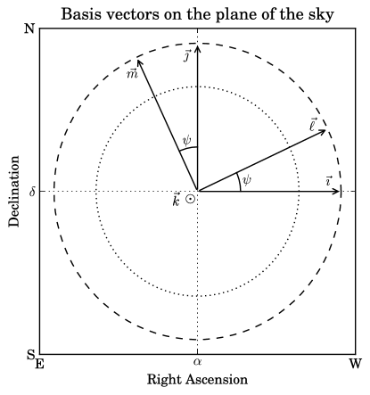
Figure 1: Basis vectors used to define the basis tensors, from the perspective of the observer looking at the source. The propagation unit vector $\vec{k}$ is pointing out of the page. The unit vector $\vec{\imath}$ lies in the equatorial plane perpendicular to the line of sight, pointing “West on the sky” in the direction of decreasing right ascension $\alpha$, and the unit vector $\vec{\jmath}$ points “North on the sky” in the direction of increasing declination $\delta$. They are used to construct basis tensors ${\mathchoice{\mathord{\hbox to0.0pt{\hbox to8.79988pt{\hss$\displaystyle\varepsilon$\hss}\hss}\raise 4.95134pt\hbox to8.79988pt{\hss\hbox{$\scriptstyle\leftrightarrow$}\hss}}}{\mathord{\hbox to0.0pt{\hbox to8.79988pt{\hss$\textstyle\varepsilon$\hss}\hss}\raise 4.95134pt\hbox to8.79988pt{\hss\hbox{$\scriptstyle\leftrightarrow$}\hss}}}{\mathord{\hbox to0.0pt{\hbox to6.99988pt{\hss$\scriptstyle\varepsilon$\hss}\hss}\raise 3.46594pt\hbox to6.99988pt{\hss\hbox{$\scriptscriptstyle\leftrightarrow$}\hss}}}{\mathord{\hbox to0.0pt{\hbox to6.99988pt{\hss$\scriptscriptstyle\varepsilon$\hss}\hss}\raise 2.47566pt\hbox to6.99988pt{\hss\hbox{$\scriptscriptstyle\leftrightarrow$}\hss}}}}\mathord{\hbox{}}_{\!+}=\vec{\imath}\otimes\vec{\imath}-\vec{\jmath}\otimes\vec{\jmath}$ and ${\mathchoice{\mathord{\hbox to0.0pt{\hbox to8.79988pt{\hss$\displaystyle\varepsilon$\hss}\hss}\raise 4.95134pt\hbox to8.79988pt{\hss\hbox{$\scriptstyle\leftrightarrow$}\hss}}}{\mathord{\hbox to0.0pt{\hbox to8.79988pt{\hss$\textstyle\varepsilon$\hss}\hss}\raise 4.95134pt\hbox to8.79988pt{\hss\hbox{$\scriptstyle\leftrightarrow$}\hss}}}{\mathord{\hbox to0.0pt{\hbox to6.99988pt{\hss$\scriptstyle\varepsilon$\hss}\hss}\raise 3.46594pt\hbox to6.99988pt{\hss\hbox{$\scriptscriptstyle\leftrightarrow$}\hss}}}{\mathord{\hbox to0.0pt{\hbox to6.99988pt{\hss$\scriptscriptstyle\varepsilon$\hss}\hss}\raise 2.47566pt\hbox to6.99988pt{\hss\hbox{$\scriptscriptstyle\leftrightarrow$}\hss}}}}\mathord{\hbox{}}_{\!\times}=\vec{\imath}\otimes\vec{\jmath}+\vec{\jmath}\otimes\vec{\imath}$. The source’s preferred polarization basis ${\mathchoice{\mathord{\hbox to0.0pt{\hbox to8.79988pt{\hss$\displaystyle e$\hss}\hss}\raise 4.95134pt\hbox to8.79988pt{\hss\hbox{$\scriptstyle\leftrightarrow$}\hss}}}{\mathord{\hbox to0.0pt{\hbox to8.79988pt{\hss$\textstyle e$\hss}\hss}\raise 4.95134pt\hbox to8.79988pt{\hss\hbox{$\scriptstyle\leftrightarrow$}\hss}}}{\mathord{\hbox to0.0pt{\hbox to6.99988pt{\hss$\scriptstyle e$\hss}\hss}\raise 3.46594pt\hbox to6.99988pt{\hss\hbox{$\scriptscriptstyle\leftrightarrow$}\hss}}}{\mathord{\hbox to0.0pt{\hbox to6.99988pt{\hss$\scriptscriptstyle e$\hss}\hss}\raise 2.47566pt\hbox to6.99988pt{\hss\hbox{$\scriptscriptstyle\leftrightarrow$}\hss}}}}\mathord{\hbox{}}_{\!+}=\vec{\ell}\otimes\vec{\ell}-\vec{m}\otimes\vec{m}$ and ${\mathchoice{\mathord{\hbox to0.0pt{\hbox to8.79988pt{\hss$\displaystyle e$\hss}\hss}\raise 4.95134pt\hbox to8.79988pt{\hss\hbox{$\scriptstyle\leftrightarrow$}\hss}}}{\mathord{\hbox to0.0pt{\hbox to8.79988pt{\hss$\textstyle e$\hss}\hss}\raise 4.95134pt\hbox to8.79988pt{\hss\hbox{$\scriptstyle\leftrightarrow$}\hss}}}{\mathord{\hbox to0.0pt{\hbox to6.99988pt{\hss$\scriptstyle e$\hss}\hss}\raise 3.46594pt\hbox to6.99988pt{\hss\hbox{$\scriptscriptstyle\leftrightarrow$}\hss}}}{\mathord{\hbox to0.0pt{\hbox to6.99988pt{\hss$\scriptscriptstyle e$\hss}\hss}\raise 2.47566pt\hbox to6.99988pt{\hss\hbox{$\scriptscriptstyle\leftrightarrow$}\hss}}}}\mathord{\hbox{}}_{\!\times}=\vec{\ell}\otimes\vec{m}+\vec{m}\otimes\vec{\ell}$ is defined by constructing a right-handed orthonormal basis $\{\vec{\ell},\vec{m},\vec{k}\}$ such that either $\vec{\ell}$ or $\vec{m}$ to lie parallel or antiparallel to the projection onto the sky of the neutron star spin; the other unit vector then lies in the neutron star’s equatorial plane. The polarization angle $\psi$ is measured counterclockwise from $\vec{\imath}$ to $\vec{\ell}$. By choosing $\vec{\ell}$ or $\vec{m}$ to lie parallel or antiparallel to the projected angular momentum, $\psi$ can be arranged to lie in the interval $(-\pi/4,\pi/4]$.

The angle $\psi$ is measured counter-clockwise from a reference direction $\vec{\imath}$ to $\vec{\ell}$. The freedom to choose $\vec{\ell}$ or $\vec{m}$ pointing in either direction within the orbital plane allows us to restrict $\psi$ to a 90-degree interval such as $(-\pi/4,\pi/4]$. The reference direction $\vec{\imath}$ is defined to lie in the Earth’s equatorial plane, perpendicular to the line of sight, pointing in the local “West on the sky” direction of decreasing right ascension. Together with a unit vector $\vec{\jmath}$ pointing “North on the sky” (perpendicular to the line of sight, in the direction of increasing declination), it forms a right-handed orthonormal basis $\{\vec{\imath},\vec{\jmath},\vec{k}\}$. We can use this basis to form an alternate set of basis tensors

$${\mathchoice{\mathord{\hbox to0.0pt{\hbox to8.79988pt{\hss$\displaystyle\varepsilon$\hss}\hss}\raise 4.95134pt\hbox to8.79988pt{\hss\hbox{$\scriptstyle\leftrightarrow$}\hss}}}{\mathord{\hbox to0.0pt{\hbox to8.79988pt{\hss$\textstyle\varepsilon$\hss}\hss}\raise 4.95134pt\hbox to8.79988pt{\hss\hbox{$\scriptstyle\leftrightarrow$}\hss}}}{\mathord{\hbox to0.0pt{\hbox to6.99988pt{\hss$\scriptstyle\varepsilon$\hss}\hss}\raise 3.46594pt\hbox to6.99988pt{\hss\hbox{$\scriptscriptstyle\leftrightarrow$}\hss}}}{\mathord{\hbox to0.0pt{\hbox to6.99988pt{\hss$\scriptscriptstyle\varepsilon$\hss}\hss}\raise 2.47566pt\hbox to6.99988pt{\hss\hbox{$\scriptscriptstyle\leftrightarrow$}\hss}}}}\mathord{\hbox{}}_{\!+} =\vec{\imath}\otimes\vec{\imath}-\vec{\jmath}\otimes\vec{\jmath}$$ (4a)

$${\mathchoice{\mathord{\hbox to0.0pt{\hbox to8.79988pt{\hss$\displaystyle\varepsilon$\hss}\hss}\raise 4.95134pt\hbox to8.79988pt{\hss\hbox{$\scriptstyle\leftrightarrow$}\hss}}}{\mathord{\hbox to0.0pt{\hbox to8.79988pt{\hss$\textstyle\varepsilon$\hss}\hss}\raise 4.95134pt\hbox to8.79988pt{\hss\hbox{$\scriptstyle\leftrightarrow$}\hss}}}{\mathord{\hbox to0.0pt{\hbox to6.99988pt{\hss$\scriptstyle\varepsilon$\hss}\hss}\raise 3.46594pt\hbox to6.99988pt{\hss\hbox{$\scriptscriptstyle\leftrightarrow$}\hss}}}{\mathord{\hbox to0.0pt{\hbox to6.99988pt{\hss$\scriptscriptstyle\varepsilon$\hss}\hss}\raise 2.47566pt\hbox to6.99988pt{\hss\hbox{$\scriptscriptstyle\leftrightarrow$}\hss}}}}\mathord{\hbox{}}_{\!\times} =\vec{\imath}\otimes\vec{\jmath}+\vec{\jmath}\otimes\vec{\imath}$$ (4b)

which are determined entirely by the sky position $\{\alpha,\delta\}$. In terms of this alternate polarization basis, the preferred basis can be written as

$${\mathchoice{\mathord{\hbox to0.0pt{\hbox to8.79988pt{\hss$\displaystyle e$\hss}\hss}\raise 4.95134pt\hbox to8.79988pt{\hss\hbox{$\scriptstyle\leftrightarrow$}\hss}}}{\mathord{\hbox to0.0pt{\hbox to8.79988pt{\hss$\textstyle e$\hss}\hss}\raise 4.95134pt\hbox to8.79988pt{\hss\hbox{$\scriptstyle\leftrightarrow$}\hss}}}{\mathord{\hbox to0.0pt{\hbox to6.99988pt{\hss$\scriptstyle e$\hss}\hss}\raise 3.46594pt\hbox to6.99988pt{\hss\hbox{$\scriptscriptstyle\leftrightarrow$}\hss}}}{\mathord{\hbox to0.0pt{\hbox to6.99988pt{\hss$\scriptscriptstyle e$\hss}\hss}\raise 2.47566pt\hbox to6.99988pt{\hss\hbox{$\scriptscriptstyle\leftrightarrow$}\hss}}}}\mathord{\hbox{}}_{\!+}\, = {\mathchoice{\mathord{\hbox to0.0pt{\hbox to8.79988pt{\hss$\displaystyle\varepsilon$\hss}\hss}\raise 4.95134pt\hbox to8.79988pt{\hss\hbox{$\scriptstyle\leftrightarrow$}\hss}}}{\mathord{\hbox to0.0pt{\hbox to8.79988pt{\hss$\textstyle\varepsilon$\hss}\hss}\raise 4.95134pt\hbox to8.79988pt{\hss\hbox{$\scriptstyle\leftrightarrow$}\hss}}}{\mathord{\hbox to0.0pt{\hbox to6.99988pt{\hss$\scriptstyle\varepsilon$\hss}\hss}\raise 3.46594pt\hbox to6.99988pt{\hss\hbox{$\scriptscriptstyle\leftrightarrow$}\hss}}}{\mathord{\hbox to0.0pt{\hbox to6.99988pt{\hss$\scriptscriptstyle\varepsilon$\hss}\hss}\raise 2.47566pt\hbox to6.99988pt{\hss\hbox{$\scriptscriptstyle\leftrightarrow$}\hss}}}}\mathord{\hbox{}}_{\!+} \,\cos 2\psi\, + \,{\mathchoice{\mathord{\hbox to0.0pt{\hbox to8.79988pt{\hss$\displaystyle\varepsilon$\hss}\hss}\raise 4.95134pt\hbox to8.79988pt{\hss\hbox{$\scriptstyle\leftrightarrow$}\hss}}}{\mathord{\hbox to0.0pt{\hbox to8.79988pt{\hss$\textstyle\varepsilon$\hss}\hss}\raise 4.95134pt\hbox to8.79988pt{\hss\hbox{$\scriptstyle\leftrightarrow$}\hss}}}{\mathord{\hbox to0.0pt{\hbox to6.99988pt{\hss$\scriptstyle\varepsilon$\hss}\hss}\raise 3.46594pt\hbox to6.99988pt{\hss\hbox{$\scriptscriptstyle\leftrightarrow$}\hss}}}{\mathord{\hbox to0.0pt{\hbox to6.99988pt{\hss$\scriptscriptstyle\varepsilon$\hss}\hss}\raise 2.47566pt\hbox to6.99988pt{\hss\hbox{$\scriptscriptstyle\leftrightarrow$}\hss}}}}\mathord{\hbox{}}_{\!\times}\,\sin 2\psi$$ (5a)

$${\mathchoice{\mathord{\hbox to0.0pt{\hbox to8.79988pt{\hss$\displaystyle e$\hss}\hss}\raise 4.95134pt\hbox to8.79988pt{\hss\hbox{$\scriptstyle\leftrightarrow$}\hss}}}{\mathord{\hbox to0.0pt{\hbox to8.79988pt{\hss$\textstyle e$\hss}\hss}\raise 4.95134pt\hbox to8.79988pt{\hss\hbox{$\scriptstyle\leftrightarrow$}\hss}}}{\mathord{\hbox to0.0pt{\hbox to6.99988pt{\hss$\scriptstyle e$\hss}\hss}\raise 3.46594pt\hbox to6.99988pt{\hss\hbox{$\scriptscriptstyle\leftrightarrow$}\hss}}}{\mathord{\hbox to0.0pt{\hbox to6.99988pt{\hss$\scriptscriptstyle e$\hss}\hss}\raise 2.47566pt\hbox to6.99988pt{\hss\hbox{$\scriptscriptstyle\leftrightarrow$}\hss}}}}\mathord{\hbox{}}_{\!\times}\, =-\, {\mathchoice{\mathord{\hbox to0.0pt{\hbox to8.79988pt{\hss$\displaystyle\varepsilon$\hss}\hss}\raise 4.95134pt\hbox to8.79988pt{\hss\hbox{$\scriptstyle\leftrightarrow$}\hss}}}{\mathord{\hbox to0.0pt{\hbox to8.79988pt{\hss$\textstyle\varepsilon$\hss}\hss}\raise 4.95134pt\hbox to8.79988pt{\hss\hbox{$\scriptstyle\leftrightarrow$}\hss}}}{\mathord{\hbox to0.0pt{\hbox to6.99988pt{\hss$\scriptstyle\varepsilon$\hss}\hss}\raise 3.46594pt\hbox to6.99988pt{\hss\hbox{$\scriptscriptstyle\leftrightarrow$}\hss}}}{\mathord{\hbox to0.0pt{\hbox to6.99988pt{\hss$\scriptscriptstyle\varepsilon$\hss}\hss}\raise 2.47566pt\hbox to6.99988pt{\hss\hbox{$\scriptscriptstyle\leftrightarrow$}\hss}}}}\mathord{\hbox{}}_{\!+} \,\sin 2\psi\, + \,{\mathchoice{\mathord{\hbox to0.0pt{\hbox to8.79988pt{\hss$\displaystyle\varepsilon$\hss}\hss}\raise 4.95134pt\hbox to8.79988pt{\hss\hbox{$\scriptstyle\leftrightarrow$}\hss}}}{\mathord{\hbox to0.0pt{\hbox to8.79988pt{\hss$\textstyle\varepsilon$\hss}\hss}\raise 4.95134pt\hbox to8.79988pt{\hss\hbox{$\scriptstyle\leftrightarrow$}\hss}}}{\mathord{\hbox to0.0pt{\hbox to6.99988pt{\hss$\scriptstyle\varepsilon$\hss}\hss}\raise 3.46594pt\hbox to6.99988pt{\hss\hbox{$\scriptscriptstyle\leftrightarrow$}\hss}}}{\mathord{\hbox to0.0pt{\hbox to6.99988pt{\hss$\scriptscriptstyle\varepsilon$\hss}\hss}\raise 2.47566pt\hbox to6.99988pt{\hss\hbox{$\scriptscriptstyle\leftrightarrow$}\hss}}}}\mathord{\hbox{}}_{\!\times}\,\cos 2\psi\ .$$ (5b)

For GWs generated by a non-precessing system with nearly periodically varying quadrupole moments (e.g., a triaxial neutron star spinning about a principal axis), the amplitudes of the two polarizations are given by

$$A_{+} =\frac{h_{0}}{2}(1+\cos^{2}\iota)$$ (6a)

$$A_{\times} =h_{0}\cos\iota\ ,$$ (6b)

where $\iota$ is the angle between the line of sight and the neutron star’s rotation axis, and

$$h_{0}=\frac{4G}{c^{4}}\frac{\left\lvert I_{xx}-I_{yy}\right\rvert\Omega^{2}}{d}$$ (7)

is the amplitude in terms of the equatorial quadrupole moments $\{I_{xx},I_{yy}\}$, the rotation frequency $\Omega$, and the distance $d$ to the source.

Finally, the phase evolution $\phi(\tau)$ at the SSB is typically described in terms of parameters describing the neutron star rotation and spindown, e.g.,

$$\phi(\tau)=2\pi\left(f_{0}\tau+f_{1}\frac{\tau^{2}}{2}+\cdots\right)\ ,$$ (8)

although it may be more complicated if, e.g., the spinning neutron star is in a binary system which Doppler modulates the signal.

The parameters describing the signal are divided into two categories:

• Amplitude parameters $\{h_{0},\iota,\psi,\phi_{0}\}$, and

• Phase-evolution parameters such as the sky position $\{\alpha,\delta\}$, signal frequency and spindown parameters ${f_{0},f_{1},\ldots}$, and any orbital parameters for spinning neutron stars in binary systems.

Finally, the measured signal $h^{X}(t)$ at time $t$ by detector $X$ is the response of the detector to the GW tensor ${\mathchoice{\mathord{\hbox to0.0pt{\hbox to8.79988pt{\hss$\displaystyle h$\hss}\hss}\raise 7.98605pt\hbox to8.79988pt{\hss\hbox{$\scriptstyle\leftrightarrow$}\hss}}}{\mathord{\hbox to0.0pt{\hbox to8.79988pt{\hss$\textstyle h$\hss}\hss}\raise 7.98605pt\hbox to8.79988pt{\hss\hbox{$\scriptstyle\leftrightarrow$}\hss}}}{\mathord{\hbox to0.0pt{\hbox to6.99988pt{\hss$\scriptstyle h$\hss}\hss}\raise 5.59023pt\hbox to6.99988pt{\hss\hbox{$\scriptscriptstyle\leftrightarrow$}\hss}}}{\mathord{\hbox to0.0pt{\hbox to6.99988pt{\hss$\scriptscriptstyle h$\hss}\hss}\raise 3.99301pt\hbox to6.99988pt{\hss\hbox{$\scriptscriptstyle\leftrightarrow$}\hss}}}}\mathord{\hbox{}}^{X}(t)\equiv{\mathchoice{\mathord{\hbox to0.0pt{\hbox to8.79988pt{\hss$\displaystyle h$\hss}\hss}\raise 7.98605pt\hbox to8.79988pt{\hss\hbox{$\scriptstyle\leftrightarrow$}\hss}}}{\mathord{\hbox to0.0pt{\hbox to8.79988pt{\hss$\textstyle h$\hss}\hss}\raise 7.98605pt\hbox to8.79988pt{\hss\hbox{$\scriptstyle\leftrightarrow$}\hss}}}{\mathord{\hbox to0.0pt{\hbox to6.99988pt{\hss$\scriptstyle h$\hss}\hss}\raise 5.59023pt\hbox to6.99988pt{\hss\hbox{$\scriptscriptstyle\leftrightarrow$}\hss}}}{\mathord{\hbox to0.0pt{\hbox to6.99988pt{\hss$\scriptscriptstyle h$\hss}\hss}\raise 3.99301pt\hbox to6.99988pt{\hss\hbox{$\scriptscriptstyle\leftrightarrow$}\hss}}}}\mathord{\hbox{}}(\tau^{X}(t))$. The function $\tau^{X}(t)$ denotes the SSB arrival time $\tau$ of a wavefront that reaches detector $X$ at time $t$, which accounts for the sky-position $\{\alpha,\delta\}$ dependent Doppler modulation due to detector motion.

If we consider a stretch of time that is short enough for the detector arms to have approximately constant orientation, then we can most easily write the general detector response in the frequency domain (see for example Rubbo:2003ap ; WhelanPrix08:_MLDC1B ) as

$$\begin{split}\widetilde{h}^{X}(f)&=\widetilde{{\mathchoice{\mathord{\hbox to0.0pt{\hbox to8.79988pt{\hss$\displaystyle h$\hss}\hss}\raise 7.98605pt\hbox to8.79988pt{\hss\hbox{$\scriptstyle\leftrightarrow$}\hss}}}{\mathord{\hbox to0.0pt{\hbox to8.79988pt{\hss$\textstyle h$\hss}\hss}\raise 7.98605pt\hbox to8.79988pt{\hss\hbox{$\scriptstyle\leftrightarrow$}\hss}}}{\mathord{\hbox to0.0pt{\hbox to6.99988pt{\hss$\scriptstyle h$\hss}\hss}\raise 5.59023pt\hbox to6.99988pt{\hss\hbox{$\scriptscriptstyle\leftrightarrow$}\hss}}}{\mathord{\hbox to0.0pt{\hbox to6.99988pt{\hss$\scriptscriptstyle h$\hss}\hss}\raise 3.99301pt\hbox to6.99988pt{\hss\hbox{$\scriptscriptstyle\leftrightarrow$}\hss}}}}\mathord{\hbox{}}}{}^{X}(f):{\mathchoice{\mathord{\hbox to0.0pt{\hbox to8.79988pt{\hss$\displaystyle d$\hss}\hss}\raise 7.98605pt\hbox to8.79988pt{\hss\hbox{$\scriptstyle\leftrightarrow$}\hss}}}{\mathord{\hbox to0.0pt{\hbox to8.79988pt{\hss$\textstyle d$\hss}\hss}\raise 7.98605pt\hbox to8.79988pt{\hss\hbox{$\scriptstyle\leftrightarrow$}\hss}}}{\mathord{\hbox to0.0pt{\hbox to6.99988pt{\hss$\scriptstyle d$\hss}\hss}\raise 5.59023pt\hbox to6.99988pt{\hss\hbox{$\scriptscriptstyle\leftrightarrow$}\hss}}}{\mathord{\hbox to0.0pt{\hbox to6.99988pt{\hss$\scriptscriptstyle d$\hss}\hss}\raise 3.99301pt\hbox to6.99988pt{\hss\hbox{$\scriptscriptstyle\leftrightarrow$}\hss}}}}\mathord{\hbox{}}^{X}(f)\\ &=\widetilde{h}_{+}^{X}(f)\,F_{+}^{X}(f)+\widetilde{h}_{\times}^{X}(f)\,F_{\times}^{X}(f)\ ,\end{split}$$ (9)

where $\widetilde{\;\;\;}$ denotes the Fourier-transform, and the antenna pattern functions are defined as

$$F_{+}^{X}(f) \equiv{\mathchoice{\mathord{\hbox to0.0pt{\hbox to8.79988pt{\hss$\displaystyle e$\hss}\hss}\raise 4.95134pt\hbox to8.79988pt{\hss\hbox{$\scriptstyle\leftrightarrow$}\hss}}}{\mathord{\hbox to0.0pt{\hbox to8.79988pt{\hss$\textstyle e$\hss}\hss}\raise 4.95134pt\hbox to8.79988pt{\hss\hbox{$\scriptstyle\leftrightarrow$}\hss}}}{\mathord{\hbox to0.0pt{\hbox to6.99988pt{\hss$\scriptstyle e$\hss}\hss}\raise 3.46594pt\hbox to6.99988pt{\hss\hbox{$\scriptscriptstyle\leftrightarrow$}\hss}}}{\mathord{\hbox to0.0pt{\hbox to6.99988pt{\hss$\scriptscriptstyle e$\hss}\hss}\raise 2.47566pt\hbox to6.99988pt{\hss\hbox{$\scriptscriptstyle\leftrightarrow$}\hss}}}}\mathord{\hbox{}}_{\!+}:{\mathchoice{\mathord{\hbox to0.0pt{\hbox to8.79988pt{\hss$\displaystyle d$\hss}\hss}\raise 7.98605pt\hbox to8.79988pt{\hss\hbox{$\scriptstyle\leftrightarrow$}\hss}}}{\mathord{\hbox to0.0pt{\hbox to8.79988pt{\hss$\textstyle d$\hss}\hss}\raise 7.98605pt\hbox to8.79988pt{\hss\hbox{$\scriptstyle\leftrightarrow$}\hss}}}{\mathord{\hbox to0.0pt{\hbox to6.99988pt{\hss$\scriptstyle d$\hss}\hss}\raise 5.59023pt\hbox to6.99988pt{\hss\hbox{$\scriptscriptstyle\leftrightarrow$}\hss}}}{\mathord{\hbox to0.0pt{\hbox to6.99988pt{\hss$\scriptscriptstyle d$\hss}\hss}\raise 3.99301pt\hbox to6.99988pt{\hss\hbox{$\scriptscriptstyle\leftrightarrow$}\hss}}}}\mathord{\hbox{}}^{X}(f)\ ,$$ (10a)

$$F_{\times}^{X}(f) \equiv{\mathchoice{\mathord{\hbox to0.0pt{\hbox to8.79988pt{\hss$\displaystyle e$\hss}\hss}\raise 4.95134pt\hbox to8.79988pt{\hss\hbox{$\scriptstyle\leftrightarrow$}\hss}}}{\mathord{\hbox to0.0pt{\hbox to8.79988pt{\hss$\textstyle e$\hss}\hss}\raise 4.95134pt\hbox to8.79988pt{\hss\hbox{$\scriptstyle\leftrightarrow$}\hss}}}{\mathord{\hbox to0.0pt{\hbox to6.99988pt{\hss$\scriptstyle e$\hss}\hss}\raise 3.46594pt\hbox to6.99988pt{\hss\hbox{$\scriptscriptstyle\leftrightarrow$}\hss}}}{\mathord{\hbox to0.0pt{\hbox to6.99988pt{\hss$\scriptscriptstyle e$\hss}\hss}\raise 2.47566pt\hbox to6.99988pt{\hss\hbox{$\scriptscriptstyle\leftrightarrow$}\hss}}}}\mathord{\hbox{}}_{\!\times}:{\mathchoice{\mathord{\hbox to0.0pt{\hbox to8.79988pt{\hss$\displaystyle d$\hss}\hss}\raise 7.98605pt\hbox to8.79988pt{\hss\hbox{$\scriptstyle\leftrightarrow$}\hss}}}{\mathord{\hbox to0.0pt{\hbox to8.79988pt{\hss$\textstyle d$\hss}\hss}\raise 7.98605pt\hbox to8.79988pt{\hss\hbox{$\scriptstyle\leftrightarrow$}\hss}}}{\mathord{\hbox to0.0pt{\hbox to6.99988pt{\hss$\scriptstyle d$\hss}\hss}\raise 5.59023pt\hbox to6.99988pt{\hss\hbox{$\scriptscriptstyle\leftrightarrow$}\hss}}}{\mathord{\hbox to0.0pt{\hbox to6.99988pt{\hss$\scriptscriptstyle d$\hss}\hss}\raise 3.99301pt\hbox to6.99988pt{\hss\hbox{$\scriptscriptstyle\leftrightarrow$}\hss}}}}\mathord{\hbox{}}^{X}(f)\ ,$$ (10b)

in terms of the (generally complex, and sky-position dependent) detector tensor ${\mathchoice{\mathord{\hbox to0.0pt{\hbox to8.79988pt{\hss$\displaystyle d$\hss}\hss}\raise 7.98605pt\hbox to8.79988pt{\hss\hbox{$\scriptstyle\leftrightarrow$}\hss}}}{\mathord{\hbox to0.0pt{\hbox to8.79988pt{\hss$\textstyle d$\hss}\hss}\raise 7.98605pt\hbox to8.79988pt{\hss\hbox{$\scriptstyle\leftrightarrow$}\hss}}}{\mathord{\hbox to0.0pt{\hbox to6.99988pt{\hss$\scriptstyle d$\hss}\hss}\raise 5.59023pt\hbox to6.99988pt{\hss\hbox{$\scriptscriptstyle\leftrightarrow$}\hss}}}{\mathord{\hbox to0.0pt{\hbox to6.99988pt{\hss$\scriptscriptstyle d$\hss}\hss}\raise 3.99301pt\hbox to6.99988pt{\hss\hbox{$\scriptscriptstyle\leftrightarrow$}\hss}}}}\mathord{\hbox{}}^{X}(f)$. Along the lines of (5), the dependence of $\{F_{+},F_{\times}\}$ upon the sky position and the polarization basis can be separated as

$$F_{+}(\alpha,\delta,\psi)\, = a(\alpha,\delta) \,\cos 2\psi\, + \,b(\alpha,\delta)\,\sin 2\psi\ ,$$ (11a)

$$F_{\times}(\alpha,\delta,\psi)\, =-\, a(\alpha,\delta) \,\sin 2\psi\, + \,b(\alpha,\delta)\,\cos 2\psi\ ,$$ (11b)

in terms of the (generally complex) amplitude modulation coefficients

$$a^{X}(f) \equiv{\mathchoice{\mathord{\hbox to0.0pt{\hbox to8.79988pt{\hss$\displaystyle\varepsilon$\hss}\hss}\raise 4.95134pt\hbox to8.79988pt{\hss\hbox{$\scriptstyle\leftrightarrow$}\hss}}}{\mathord{\hbox to0.0pt{\hbox to8.79988pt{\hss$\textstyle\varepsilon$\hss}\hss}\raise 4.95134pt\hbox to8.79988pt{\hss\hbox{$\scriptstyle\leftrightarrow$}\hss}}}{\mathord{\hbox to0.0pt{\hbox to6.99988pt{\hss$\scriptstyle\varepsilon$\hss}\hss}\raise 3.46594pt\hbox to6.99988pt{\hss\hbox{$\scriptscriptstyle\leftrightarrow$}\hss}}}{\mathord{\hbox to0.0pt{\hbox to6.99988pt{\hss$\scriptscriptstyle\varepsilon$\hss}\hss}\raise 2.47566pt\hbox to6.99988pt{\hss\hbox{$\scriptscriptstyle\leftrightarrow$}\hss}}}}\mathord{\hbox{}}_{\!+}:{\mathchoice{\mathord{\hbox to0.0pt{\hbox to8.79988pt{\hss$\displaystyle d$\hss}\hss}\raise 7.98605pt\hbox to8.79988pt{\hss\hbox{$\scriptstyle\leftrightarrow$}\hss}}}{\mathord{\hbox to0.0pt{\hbox to8.79988pt{\hss$\textstyle d$\hss}\hss}\raise 7.98605pt\hbox to8.79988pt{\hss\hbox{$\scriptstyle\leftrightarrow$}\hss}}}{\mathord{\hbox to0.0pt{\hbox to6.99988pt{\hss$\scriptstyle d$\hss}\hss}\raise 5.59023pt\hbox to6.99988pt{\hss\hbox{$\scriptscriptstyle\leftrightarrow$}\hss}}}{\mathord{\hbox to0.0pt{\hbox to6.99988pt{\hss$\scriptscriptstyle d$\hss}\hss}\raise 3.99301pt\hbox to6.99988pt{\hss\hbox{$\scriptscriptstyle\leftrightarrow$}\hss}}}}\mathord{\hbox{}}^{X}(f)\ ,$$ (12a)

$$b^{X}(f) \equiv{\mathchoice{\mathord{\hbox to0.0pt{\hbox to8.79988pt{\hss$\displaystyle\varepsilon$\hss}\hss}\raise 4.95134pt\hbox to8.79988pt{\hss\hbox{$\scriptstyle\leftrightarrow$}\hss}}}{\mathord{\hbox to0.0pt{\hbox to8.79988pt{\hss$\textstyle\varepsilon$\hss}\hss}\raise 4.95134pt\hbox to8.79988pt{\hss\hbox{$\scriptstyle\leftrightarrow$}\hss}}}{\mathord{\hbox to0.0pt{\hbox to6.99988pt{\hss$\scriptstyle\varepsilon$\hss}\hss}\raise 3.46594pt\hbox to6.99988pt{\hss\hbox{$\scriptscriptstyle\leftrightarrow$}\hss}}}{\mathord{\hbox to0.0pt{\hbox to6.99988pt{\hss$\scriptscriptstyle\varepsilon$\hss}\hss}\raise 2.47566pt\hbox to6.99988pt{\hss\hbox{$\scriptscriptstyle\leftrightarrow$}\hss}}}}\mathord{\hbox{}}_{\!\times}:{\mathchoice{\mathord{\hbox to0.0pt{\hbox to8.79988pt{\hss$\displaystyle d$\hss}\hss}\raise 7.98605pt\hbox to8.79988pt{\hss\hbox{$\scriptstyle\leftrightarrow$}\hss}}}{\mathord{\hbox to0.0pt{\hbox to8.79988pt{\hss$\textstyle d$\hss}\hss}\raise 7.98605pt\hbox to8.79988pt{\hss\hbox{$\scriptstyle\leftrightarrow$}\hss}}}{\mathord{\hbox to0.0pt{\hbox to6.99988pt{\hss$\scriptstyle d$\hss}\hss}\raise 5.59023pt\hbox to6.99988pt{\hss\hbox{$\scriptscriptstyle\leftrightarrow$}\hss}}}{\mathord{\hbox to0.0pt{\hbox to6.99988pt{\hss$\scriptscriptstyle d$\hss}\hss}\raise 3.99301pt\hbox to6.99988pt{\hss\hbox{$\scriptscriptstyle\leftrightarrow$}\hss}}}}\mathord{\hbox{}}^{X}(f)\ ,$$ (12b)

which are independent of the signal amplitude parameters.

In the case of ground-based detectors, one commonly uses the long-wavelength limit approximation, as the interferometer arms are typically much shorter than the wavelength $c/f_{0}$ of the GWs. In this limit the detector-response tensor ${\mathchoice{\mathord{\hbox to0.0pt{\hbox to8.79988pt{\hss$\displaystyle d$\hss}\hss}\raise 7.98605pt\hbox to8.79988pt{\hss\hbox{$\scriptstyle\leftrightarrow$}\hss}}}{\mathord{\hbox to0.0pt{\hbox to8.79988pt{\hss$\textstyle d$\hss}\hss}\raise 7.98605pt\hbox to8.79988pt{\hss\hbox{$\scriptstyle\leftrightarrow$}\hss}}}{\mathord{\hbox to0.0pt{\hbox to6.99988pt{\hss$\scriptstyle d$\hss}\hss}\raise 5.59023pt\hbox to6.99988pt{\hss\hbox{$\scriptscriptstyle\leftrightarrow$}\hss}}}{\mathord{\hbox to0.0pt{\hbox to6.99988pt{\hss$\scriptscriptstyle d$\hss}\hss}\raise 3.99301pt\hbox to6.99988pt{\hss\hbox{$\scriptscriptstyle\leftrightarrow$}\hss}}}}\mathord{\hbox{}}(f)$ becomes real-valued and independent of frequency (and sky-position), and can be expressed as

$${\mathchoice{\mathord{\hbox to0.0pt{\hbox to8.79988pt{\hss$\displaystyle d$\hss}\hss}\raise 7.98605pt\hbox to8.79988pt{\hss\hbox{$\scriptstyle\leftrightarrow$}\hss}}}{\mathord{\hbox to0.0pt{\hbox to8.79988pt{\hss$\textstyle d$\hss}\hss}\raise 7.98605pt\hbox to8.79988pt{\hss\hbox{$\scriptstyle\leftrightarrow$}\hss}}}{\mathord{\hbox to0.0pt{\hbox to6.99988pt{\hss$\scriptstyle d$\hss}\hss}\raise 5.59023pt\hbox to6.99988pt{\hss\hbox{$\scriptscriptstyle\leftrightarrow$}\hss}}}{\mathord{\hbox to0.0pt{\hbox to6.99988pt{\hss$\scriptscriptstyle d$\hss}\hss}\raise 3.99301pt\hbox to6.99988pt{\hss\hbox{$\scriptscriptstyle\leftrightarrow$}\hss}}}}\mathord{\hbox{}}(f)\approx{\mathchoice{\mathord{\hbox to0.0pt{\hbox to8.79988pt{\hss$\displaystyle d$\hss}\hss}\raise 7.98605pt\hbox to8.79988pt{\hss\hbox{$\scriptstyle\leftrightarrow$}\hss}}}{\mathord{\hbox to0.0pt{\hbox to8.79988pt{\hss$\textstyle d$\hss}\hss}\raise 7.98605pt\hbox to8.79988pt{\hss\hbox{$\scriptstyle\leftrightarrow$}\hss}}}{\mathord{\hbox to0.0pt{\hbox to6.99988pt{\hss$\scriptstyle d$\hss}\hss}\raise 5.59023pt\hbox to6.99988pt{\hss\hbox{$\scriptscriptstyle\leftrightarrow$}\hss}}}{\mathord{\hbox to0.0pt{\hbox to6.99988pt{\hss$\scriptscriptstyle d$\hss}\hss}\raise 3.99301pt\hbox to6.99988pt{\hss\hbox{$\scriptscriptstyle\leftrightarrow$}\hss}}}}\mathord{\hbox{}}_{\mathrm{LWL}}\equiv\frac{1}{2}\left(\vec{u}\otimes\vec{u}+\vec{v}\otimes\vec{v}\right)\ ,$$ (13)

for interferometer arms along unit vectors $\vec{u}$ and $\vec{v}$.

III Coordinates on Amplitude Parameter Space

III.1 Physical Coordinates

The amplitude parameters most closely connected to the geometry of the emitting system are $\{h_{0},\iota,\psi,\phi_{0}\}$. They form a set of coordinates on the four-dimensional amplitude parameter space. Any signal of the form (1) can be described by parameters in the range

$$0\leq h_{0}<\infty\qquad\hbox{and}\qquad 0\leq\iota\leq\pi$$ (14)

and

$$-\frac{\pi}{4}<\psi\leq\frac{\pi}{4}\qquad\hbox{and}\qquad 0\leq\phi_{0}<2\pi$$ (15)

The range of angles can be understood by noting that if we make the transformation $\psi\rightarrow\psi+\pi/2$, (5) implies that $\{{\mathchoice{\mathord{\hbox to0.0pt{\hbox to8.79988pt{\hss$\displaystyle e$\hss}\hss}\raise 4.95134pt\hbox to8.79988pt{\hss\hbox{$\scriptstyle\leftrightarrow$}\hss}}}{\mathord{\hbox to0.0pt{\hbox to8.79988pt{\hss$\textstyle e$\hss}\hss}\raise 4.95134pt\hbox to8.79988pt{\hss\hbox{$\scriptstyle\leftrightarrow$}\hss}}}{\mathord{\hbox to0.0pt{\hbox to6.99988pt{\hss$\scriptstyle e$\hss}\hss}\raise 3.46594pt\hbox to6.99988pt{\hss\hbox{$\scriptscriptstyle\leftrightarrow$}\hss}}}{\mathord{\hbox to0.0pt{\hbox to6.99988pt{\hss$\scriptscriptstyle e$\hss}\hss}\raise 2.47566pt\hbox to6.99988pt{\hss\hbox{$\scriptscriptstyle\leftrightarrow$}\hss}}}}\mathord{\hbox{}}_{\!+},{\mathchoice{\mathord{\hbox to0.0pt{\hbox to8.79988pt{\hss$\displaystyle e$\hss}\hss}\raise 4.95134pt\hbox to8.79988pt{\hss\hbox{$\scriptstyle\leftrightarrow$}\hss}}}{\mathord{\hbox to0.0pt{\hbox to8.79988pt{\hss$\textstyle e$\hss}\hss}\raise 4.95134pt\hbox to8.79988pt{\hss\hbox{$\scriptstyle\leftrightarrow$}\hss}}}{\mathord{\hbox to0.0pt{\hbox to6.99988pt{\hss$\scriptstyle e$\hss}\hss}\raise 3.46594pt\hbox to6.99988pt{\hss\hbox{$\scriptscriptstyle\leftrightarrow$}\hss}}}{\mathord{\hbox to0.0pt{\hbox to6.99988pt{\hss$\scriptscriptstyle e$\hss}\hss}\raise 2.47566pt\hbox to6.99988pt{\hss\hbox{$\scriptscriptstyle\leftrightarrow$}\hss}}}}\mathord{\hbox{}}_{\!\times}\}\rightarrow\{-{\mathchoice{\mathord{\hbox to0.0pt{\hbox to8.79988pt{\hss$\displaystyle e$\hss}\hss}\raise 4.95134pt\hbox to8.79988pt{\hss\hbox{$\scriptstyle\leftrightarrow$}\hss}}}{\mathord{\hbox to0.0pt{\hbox to8.79988pt{\hss$\textstyle e$\hss}\hss}\raise 4.95134pt\hbox to8.79988pt{\hss\hbox{$\scriptstyle\leftrightarrow$}\hss}}}{\mathord{\hbox to0.0pt{\hbox to6.99988pt{\hss$\scriptstyle e$\hss}\hss}\raise 3.46594pt\hbox to6.99988pt{\hss\hbox{$\scriptscriptstyle\leftrightarrow$}\hss}}}{\mathord{\hbox to0.0pt{\hbox to6.99988pt{\hss$\scriptscriptstyle e$\hss}\hss}\raise 2.47566pt\hbox to6.99988pt{\hss\hbox{$\scriptscriptstyle\leftrightarrow$}\hss}}}}\mathord{\hbox{}}_{\!+},-{\mathchoice{\mathord{\hbox to0.0pt{\hbox to8.79988pt{\hss$\displaystyle e$\hss}\hss}\raise 4.95134pt\hbox to8.79988pt{\hss\hbox{$\scriptstyle\leftrightarrow$}\hss}}}{\mathord{\hbox to0.0pt{\hbox to8.79988pt{\hss$\textstyle e$\hss}\hss}\raise 4.95134pt\hbox to8.79988pt{\hss\hbox{$\scriptstyle\leftrightarrow$}\hss}}}{\mathord{\hbox to0.0pt{\hbox to6.99988pt{\hss$\scriptstyle e$\hss}\hss}\raise 3.46594pt\hbox to6.99988pt{\hss\hbox{$\scriptscriptstyle\leftrightarrow$}\hss}}}{\mathord{\hbox to0.0pt{\hbox to6.99988pt{\hss$\scriptscriptstyle e$\hss}\hss}\raise 2.47566pt\hbox to6.99988pt{\hss\hbox{$\scriptscriptstyle\leftrightarrow$}\hss}}}}\mathord{\hbox{}}_{\!\times}\}$, which means that the transformation $\{\psi,\phi_{0}\}\rightarrow\{\psi+\pi/2,\phi_{0}+\pi\}$ leaves the waveform (1) unchanged.

It is also convenient to define $\chi=\cos\iota$, so that

$$A_{+}=\frac{h_{0}}{2}(1+\chi^{2})\qquad\hbox{and}\qquad A_{\times}=h_{0}\chi$$ (16)

and consider the physical coordinates $\{h_{0},\chi\mathbin{=}\cos\iota,\psi,\phi_{0}\}$ with parameter space ranges

$$0\leq h_{0}<\infty\qquad\hbox{and}\qquad-1\leq\chi\leq 1$$ (17)

If the distribution of neutron star spins is isotropic, a physical probability distribution on amplitude parameter space should be uniform in $\chi$ and $\psi$ as well as $\phi_{0}$, so that

$$\text{pdf}(h_{0},\chi,\psi,\phi_{0}|\mathcal{H}_{s})=\frac{1}{2\pi^{2}}\text{pdf}(h_{0}|\mathcal{H}_{s})\quad\hbox{(isotropic prior)}$$ (18)

Finally, note that the range on $h_{0}$ and $\chi$ implies that

$$0\leq A_{+}<\infty\qquad\hbox{and}\qquad-A_{+}\leq A_{\times}\leq A_{+}$$ (19)

If $\iota=\pi/2$, so that $\chi=0$, the GW signal is linearly polarized. In this case, $A_{+}=h_{0}/2$, $A_{\times}=0$, and the signal in the preferred basis contains only the plus polarization state:

$$\begin{split}{\mathchoice{\mathord{\hbox to0.0pt{\hbox to8.79988pt{\hss$\displaystyle h$\hss}\hss}\raise 7.98605pt\hbox to8.79988pt{\hss\hbox{$\scriptstyle\leftrightarrow$}\hss}}}{\mathord{\hbox to0.0pt{\hbox to8.79988pt{\hss$\textstyle h$\hss}\hss}\raise 7.98605pt\hbox to8.79988pt{\hss\hbox{$\scriptstyle\leftrightarrow$}\hss}}}{\mathord{\hbox to0.0pt{\hbox to6.99988pt{\hss$\scriptstyle h$\hss}\hss}\raise 5.59023pt\hbox to6.99988pt{\hss\hbox{$\scriptscriptstyle\leftrightarrow$}\hss}}}{\mathord{\hbox to0.0pt{\hbox to6.99988pt{\hss$\scriptscriptstyle h$\hss}\hss}\raise 3.99301pt\hbox to6.99988pt{\hss\hbox{$\scriptscriptstyle\leftrightarrow$}\hss}}}}\mathord{\hbox{}}(\tau)&=\frac{h_{0}}{2}\cos(\phi(\tau)+\phi_{0}){\mathchoice{\mathord{\hbox to0.0pt{\hbox to8.79988pt{\hss$\displaystyle e$\hss}\hss}\raise 4.95134pt\hbox to8.79988pt{\hss\hbox{$\scriptstyle\leftrightarrow$}\hss}}}{\mathord{\hbox to0.0pt{\hbox to8.79988pt{\hss$\textstyle e$\hss}\hss}\raise 4.95134pt\hbox to8.79988pt{\hss\hbox{$\scriptstyle\leftrightarrow$}\hss}}}{\mathord{\hbox to0.0pt{\hbox to6.99988pt{\hss$\scriptstyle e$\hss}\hss}\raise 3.46594pt\hbox to6.99988pt{\hss\hbox{$\scriptscriptstyle\leftrightarrow$}\hss}}}{\mathord{\hbox to0.0pt{\hbox to6.99988pt{\hss$\scriptscriptstyle e$\hss}\hss}\raise 2.47566pt\hbox to6.99988pt{\hss\hbox{$\scriptscriptstyle\leftrightarrow$}\hss}}}}\mathord{\hbox{}}_{\!+}\\ &=\frac{h_{0}}{2}\cos(\phi(\tau)+\phi_{0})\left({\mathchoice{\mathord{\hbox to0.0pt{\hbox to8.79988pt{\hss$\displaystyle\varepsilon$\hss}\hss}\raise 4.95134pt\hbox to8.79988pt{\hss\hbox{$\scriptstyle\leftrightarrow$}\hss}}}{\mathord{\hbox to0.0pt{\hbox to8.79988pt{\hss$\textstyle\varepsilon$\hss}\hss}\raise 4.95134pt\hbox to8.79988pt{\hss\hbox{$\scriptstyle\leftrightarrow$}\hss}}}{\mathord{\hbox to0.0pt{\hbox to6.99988pt{\hss$\scriptstyle\varepsilon$\hss}\hss}\raise 3.46594pt\hbox to6.99988pt{\hss\hbox{$\scriptscriptstyle\leftrightarrow$}\hss}}}{\mathord{\hbox to0.0pt{\hbox to6.99988pt{\hss$\scriptscriptstyle\varepsilon$\hss}\hss}\raise 2.47566pt\hbox to6.99988pt{\hss\hbox{$\scriptscriptstyle\leftrightarrow$}\hss}}}}\mathord{\hbox{}}_{\!+}\,\cos 2\psi+{\mathchoice{\mathord{\hbox to0.0pt{\hbox to8.79988pt{\hss$\displaystyle\varepsilon$\hss}\hss}\raise 4.95134pt\hbox to8.79988pt{\hss\hbox{$\scriptstyle\leftrightarrow$}\hss}}}{\mathord{\hbox to0.0pt{\hbox to8.79988pt{\hss$\textstyle\varepsilon$\hss}\hss}\raise 4.95134pt\hbox to8.79988pt{\hss\hbox{$\scriptstyle\leftrightarrow$}\hss}}}{\mathord{\hbox to0.0pt{\hbox to6.99988pt{\hss$\scriptstyle\varepsilon$\hss}\hss}\raise 3.46594pt\hbox to6.99988pt{\hss\hbox{$\scriptscriptstyle\leftrightarrow$}\hss}}}{\mathord{\hbox to0.0pt{\hbox to6.99988pt{\hss$\scriptscriptstyle\varepsilon$\hss}\hss}\raise 2.47566pt\hbox to6.99988pt{\hss\hbox{$\scriptscriptstyle\leftrightarrow$}\hss}}}}\mathord{\hbox{}}_{\!\times}\,\sin 2\psi\right)\end{split}$$ (20)

If $\iota=0$, so that $\chi=1$, the GW signal is right circularly polarized. In this case, $A_{+}=h_{0}=A_{\times}$ and the signal is

$$\begin{split}{\mathchoice{\mathord{\hbox to0.0pt{\hbox to8.79988pt{\hss$\displaystyle h$\hss}\hss}\raise 7.98605pt\hbox to8.79988pt{\hss\hbox{$\scriptstyle\leftrightarrow$}\hss}}}{\mathord{\hbox to0.0pt{\hbox to8.79988pt{\hss$\textstyle h$\hss}\hss}\raise 7.98605pt\hbox to8.79988pt{\hss\hbox{$\scriptstyle\leftrightarrow$}\hss}}}{\mathord{\hbox to0.0pt{\hbox to6.99988pt{\hss$\scriptstyle h$\hss}\hss}\raise 5.59023pt\hbox to6.99988pt{\hss\hbox{$\scriptscriptstyle\leftrightarrow$}\hss}}}{\mathord{\hbox to0.0pt{\hbox to6.99988pt{\hss$\scriptscriptstyle h$\hss}\hss}\raise 3.99301pt\hbox to6.99988pt{\hss\hbox{$\scriptscriptstyle\leftrightarrow$}\hss}}}}\mathord{\hbox{}}(\tau)&=h_{0}\left[\cos(\phi(\tau)+\phi_{0}){\mathchoice{\mathord{\hbox to0.0pt{\hbox to8.79988pt{\hss$\displaystyle e$\hss}\hss}\raise 4.95134pt\hbox to8.79988pt{\hss\hbox{$\scriptstyle\leftrightarrow$}\hss}}}{\mathord{\hbox to0.0pt{\hbox to8.79988pt{\hss$\textstyle e$\hss}\hss}\raise 4.95134pt\hbox to8.79988pt{\hss\hbox{$\scriptstyle\leftrightarrow$}\hss}}}{\mathord{\hbox to0.0pt{\hbox to6.99988pt{\hss$\scriptstyle e$\hss}\hss}\raise 3.46594pt\hbox to6.99988pt{\hss\hbox{$\scriptscriptstyle\leftrightarrow$}\hss}}}{\mathord{\hbox to0.0pt{\hbox to6.99988pt{\hss$\scriptscriptstyle e$\hss}\hss}\raise 2.47566pt\hbox to6.99988pt{\hss\hbox{$\scriptscriptstyle\leftrightarrow$}\hss}}}}\mathord{\hbox{}}_{\!+}+\sin(\phi(\tau)+\phi_{0}){\mathchoice{\mathord{\hbox to0.0pt{\hbox to8.79988pt{\hss$\displaystyle e$\hss}\hss}\raise 4.95134pt\hbox to8.79988pt{\hss\hbox{$\scriptstyle\leftrightarrow$}\hss}}}{\mathord{\hbox to0.0pt{\hbox to8.79988pt{\hss$\textstyle e$\hss}\hss}\raise 4.95134pt\hbox to8.79988pt{\hss\hbox{$\scriptstyle\leftrightarrow$}\hss}}}{\mathord{\hbox to0.0pt{\hbox to6.99988pt{\hss$\scriptstyle e$\hss}\hss}\raise 3.46594pt\hbox to6.99988pt{\hss\hbox{$\scriptscriptstyle\leftrightarrow$}\hss}}}{\mathord{\hbox to0.0pt{\hbox to6.99988pt{\hss$\scriptscriptstyle e$\hss}\hss}\raise 2.47566pt\hbox to6.99988pt{\hss\hbox{$\scriptscriptstyle\leftrightarrow$}\hss}}}}\mathord{\hbox{}}_{\!\times}\right]\\ &=h_{0}\left[\cos(\phi(\tau)+\phi_{0}-2\psi){\mathchoice{\mathord{\hbox to0.0pt{\hbox to8.79988pt{\hss$\displaystyle\varepsilon$\hss}\hss}\raise 4.95134pt\hbox to8.79988pt{\hss\hbox{$\scriptstyle\leftrightarrow$}\hss}}}{\mathord{\hbox to0.0pt{\hbox to8.79988pt{\hss$\textstyle\varepsilon$\hss}\hss}\raise 4.95134pt\hbox to8.79988pt{\hss\hbox{$\scriptstyle\leftrightarrow$}\hss}}}{\mathord{\hbox to0.0pt{\hbox to6.99988pt{\hss$\scriptstyle\varepsilon$\hss}\hss}\raise 3.46594pt\hbox to6.99988pt{\hss\hbox{$\scriptscriptstyle\leftrightarrow$}\hss}}}{\mathord{\hbox to0.0pt{\hbox to6.99988pt{\hss$\scriptscriptstyle\varepsilon$\hss}\hss}\raise 2.47566pt\hbox to6.99988pt{\hss\hbox{$\scriptscriptstyle\leftrightarrow$}\hss}}}}\mathord{\hbox{}}_{\!+}+\sin(\phi(\tau)+\phi_{0}-2\psi){\mathchoice{\mathord{\hbox to0.0pt{\hbox to8.79988pt{\hss$\displaystyle\varepsilon$\hss}\hss}\raise 4.95134pt\hbox to8.79988pt{\hss\hbox{$\scriptstyle\leftrightarrow$}\hss}}}{\mathord{\hbox to0.0pt{\hbox to8.79988pt{\hss$\textstyle\varepsilon$\hss}\hss}\raise 4.95134pt\hbox to8.79988pt{\hss\hbox{$\scriptstyle\leftrightarrow$}\hss}}}{\mathord{\hbox to0.0pt{\hbox to6.99988pt{\hss$\scriptstyle\varepsilon$\hss}\hss}\raise 3.46594pt\hbox to6.99988pt{\hss\hbox{$\scriptscriptstyle\leftrightarrow$}\hss}}}{\mathord{\hbox to0.0pt{\hbox to6.99988pt{\hss$\scriptscriptstyle\varepsilon$\hss}\hss}\raise 2.47566pt\hbox to6.99988pt{\hss\hbox{$\scriptscriptstyle\leftrightarrow$}\hss}}}}\mathord{\hbox{}}_{\!\times}\right]\end{split}$$ (21)

We see that for right circular polarization there is a degeneracy of the $\psi$ and $\phi_{0}$ coordinates, with the waveform depending only on the combination $\phi_{0}-2\psi$.

If $\iota=\pi$, so that $\chi=-1$, the GW signal is left circularly polarized. In this case, $A_{+}=h_{0}=-A_{\times}$ and the signal is

$$\begin{split}{\mathchoice{\mathord{\hbox to0.0pt{\hbox to8.79988pt{\hss$\displaystyle h$\hss}\hss}\raise 7.98605pt\hbox to8.79988pt{\hss\hbox{$\scriptstyle\leftrightarrow$}\hss}}}{\mathord{\hbox to0.0pt{\hbox to8.79988pt{\hss$\textstyle h$\hss}\hss}\raise 7.98605pt\hbox to8.79988pt{\hss\hbox{$\scriptstyle\leftrightarrow$}\hss}}}{\mathord{\hbox to0.0pt{\hbox to6.99988pt{\hss$\scriptstyle h$\hss}\hss}\raise 5.59023pt\hbox to6.99988pt{\hss\hbox{$\scriptscriptstyle\leftrightarrow$}\hss}}}{\mathord{\hbox to0.0pt{\hbox to6.99988pt{\hss$\scriptscriptstyle h$\hss}\hss}\raise 3.99301pt\hbox to6.99988pt{\hss\hbox{$\scriptscriptstyle\leftrightarrow$}\hss}}}}\mathord{\hbox{}}(\tau)&=h_{0}\left[\cos(\phi(\tau)+\phi_{0}){\mathchoice{\mathord{\hbox to0.0pt{\hbox to8.79988pt{\hss$\displaystyle e$\hss}\hss}\raise 4.95134pt\hbox to8.79988pt{\hss\hbox{$\scriptstyle\leftrightarrow$}\hss}}}{\mathord{\hbox to0.0pt{\hbox to8.79988pt{\hss$\textstyle e$\hss}\hss}\raise 4.95134pt\hbox to8.79988pt{\hss\hbox{$\scriptstyle\leftrightarrow$}\hss}}}{\mathord{\hbox to0.0pt{\hbox to6.99988pt{\hss$\scriptstyle e$\hss}\hss}\raise 3.46594pt\hbox to6.99988pt{\hss\hbox{$\scriptscriptstyle\leftrightarrow$}\hss}}}{\mathord{\hbox to0.0pt{\hbox to6.99988pt{\hss$\scriptscriptstyle e$\hss}\hss}\raise 2.47566pt\hbox to6.99988pt{\hss\hbox{$\scriptscriptstyle\leftrightarrow$}\hss}}}}\mathord{\hbox{}}_{\!+}-\sin(\phi(\tau)+\phi_{0}){\mathchoice{\mathord{\hbox to0.0pt{\hbox to8.79988pt{\hss$\displaystyle e$\hss}\hss}\raise 4.95134pt\hbox to8.79988pt{\hss\hbox{$\scriptstyle\leftrightarrow$}\hss}}}{\mathord{\hbox to0.0pt{\hbox to8.79988pt{\hss$\textstyle e$\hss}\hss}\raise 4.95134pt\hbox to8.79988pt{\hss\hbox{$\scriptstyle\leftrightarrow$}\hss}}}{\mathord{\hbox to0.0pt{\hbox to6.99988pt{\hss$\scriptstyle e$\hss}\hss}\raise 3.46594pt\hbox to6.99988pt{\hss\hbox{$\scriptscriptstyle\leftrightarrow$}\hss}}}{\mathord{\hbox to0.0pt{\hbox to6.99988pt{\hss$\scriptscriptstyle e$\hss}\hss}\raise 2.47566pt\hbox to6.99988pt{\hss\hbox{$\scriptscriptstyle\leftrightarrow$}\hss}}}}\mathord{\hbox{}}_{\!\times}\right]\\ &=h_{0}\left[\cos(\phi(\tau)+\phi_{0}+2\psi){\mathchoice{\mathord{\hbox to0.0pt{\hbox to8.79988pt{\hss$\displaystyle\varepsilon$\hss}\hss}\raise 4.95134pt\hbox to8.79988pt{\hss\hbox{$\scriptstyle\leftrightarrow$}\hss}}}{\mathord{\hbox to0.0pt{\hbox to8.79988pt{\hss$\textstyle\varepsilon$\hss}\hss}\raise 4.95134pt\hbox to8.79988pt{\hss\hbox{$\scriptstyle\leftrightarrow$}\hss}}}{\mathord{\hbox to0.0pt{\hbox to6.99988pt{\hss$\scriptstyle\varepsilon$\hss}\hss}\raise 3.46594pt\hbox to6.99988pt{\hss\hbox{$\scriptscriptstyle\leftrightarrow$}\hss}}}{\mathord{\hbox to0.0pt{\hbox to6.99988pt{\hss$\scriptscriptstyle\varepsilon$\hss}\hss}\raise 2.47566pt\hbox to6.99988pt{\hss\hbox{$\scriptscriptstyle\leftrightarrow$}\hss}}}}\mathord{\hbox{}}_{\!+}+\sin(\phi(\tau)+\phi_{0}+2\psi){\mathchoice{\mathord{\hbox to0.0pt{\hbox to8.79988pt{\hss$\displaystyle\varepsilon$\hss}\hss}\raise 4.95134pt\hbox to8.79988pt{\hss\hbox{$\scriptstyle\leftrightarrow$}\hss}}}{\mathord{\hbox to0.0pt{\hbox to8.79988pt{\hss$\textstyle\varepsilon$\hss}\hss}\raise 4.95134pt\hbox to8.79988pt{\hss\hbox{$\scriptstyle\leftrightarrow$}\hss}}}{\mathord{\hbox to0.0pt{\hbox to6.99988pt{\hss$\scriptstyle\varepsilon$\hss}\hss}\raise 3.46594pt\hbox to6.99988pt{\hss\hbox{$\scriptscriptstyle\leftrightarrow$}\hss}}}{\mathord{\hbox to0.0pt{\hbox to6.99988pt{\hss$\scriptscriptstyle\varepsilon$\hss}\hss}\raise 2.47566pt\hbox to6.99988pt{\hss\hbox{$\scriptscriptstyle\leftrightarrow$}\hss}}}}\mathord{\hbox{}}_{\!\times}\right]\end{split}$$ (22)

We see that for right circular polarization there is a degeneracy of the $\psi$ and $\phi_{0}$ coordinates, with the waveform depending only on the combination $\phi_{0}+2\psi$.

III.2 JKS $\mathcal{A}^{\mu}$ Coordinates

The basis of the $\mathcal{F}$-statistic maximum likelihood method jks98:_data is the observation that the GW signal (1) is linear in the following four combinations of the four amplitude parameters:

$$\mathcal{A}^{1} =A_{+}\cos 2\psi\cos\phi_{0}-A_{\times}\sin 2\psi\sin\phi_{0}$$ (23a)

$$\mathcal{A}^{2} =A_{+}\sin 2\psi\cos\phi_{0}+A_{\times}\cos 2\psi\sin\phi_{0}$$ (23b)

$$\mathcal{A}^{3} =-A_{+}\cos 2\psi\sin\phi_{0}-A_{\times}\sin 2\psi\cos\phi_{0}$$ (23c)

$$\mathcal{A}^{4} =-A_{+}\sin 2\psi\sin\phi_{0}+A_{\times}\cos 2\psi\cos\phi_{0}\ .$$ (23d)

The GW tensor waveform (1) can be written as

$${\mathchoice{\mathord{\hbox to0.0pt{\hbox to8.79988pt{\hss$\displaystyle h$\hss}\hss}\raise 7.98605pt\hbox to8.79988pt{\hss\hbox{$\scriptstyle\leftrightarrow$}\hss}}}{\mathord{\hbox to0.0pt{\hbox to8.79988pt{\hss$\textstyle h$\hss}\hss}\raise 7.98605pt\hbox to8.79988pt{\hss\hbox{$\scriptstyle\leftrightarrow$}\hss}}}{\mathord{\hbox to0.0pt{\hbox to6.99988pt{\hss$\scriptstyle h$\hss}\hss}\raise 5.59023pt\hbox to6.99988pt{\hss\hbox{$\scriptscriptstyle\leftrightarrow$}\hss}}}{\mathord{\hbox to0.0pt{\hbox to6.99988pt{\hss$\scriptscriptstyle h$\hss}\hss}\raise 3.99301pt\hbox to6.99988pt{\hss\hbox{$\scriptscriptstyle\leftrightarrow$}\hss}}}}\mathord{\hbox{}}(\tau;\mathcal{A},\lambda)=\mathcal{A}^{\mu}{\mathchoice{\mathord{\hbox to0.0pt{\hbox to8.79988pt{\hss$\displaystyle h$\hss}\hss}\raise 7.98605pt\hbox to8.79988pt{\hss\hbox{$\scriptstyle\leftrightarrow$}\hss}}}{\mathord{\hbox to0.0pt{\hbox to8.79988pt{\hss$\textstyle h$\hss}\hss}\raise 7.98605pt\hbox to8.79988pt{\hss\hbox{$\scriptstyle\leftrightarrow$}\hss}}}{\mathord{\hbox to0.0pt{\hbox to6.99988pt{\hss$\scriptstyle h$\hss}\hss}\raise 5.59023pt\hbox to6.99988pt{\hss\hbox{$\scriptscriptstyle\leftrightarrow$}\hss}}}{\mathord{\hbox to0.0pt{\hbox to6.99988pt{\hss$\scriptscriptstyle h$\hss}\hss}\raise 3.99301pt\hbox to6.99988pt{\hss\hbox{$\scriptscriptstyle\leftrightarrow$}\hss}}}}\mathord{\hbox{}}_{\mu}(\tau;\lambda)\ ,$$ (24)

where

$${\mathchoice{\mathord{\hbox to0.0pt{\hbox to8.79988pt{\hss$\displaystyle h$\hss}\hss}\raise 7.98605pt\hbox to8.79988pt{\hss\hbox{$\scriptstyle\leftrightarrow$}\hss}}}{\mathord{\hbox to0.0pt{\hbox to8.79988pt{\hss$\textstyle h$\hss}\hss}\raise 7.98605pt\hbox to8.79988pt{\hss\hbox{$\scriptstyle\leftrightarrow$}\hss}}}{\mathord{\hbox to0.0pt{\hbox to6.99988pt{\hss$\scriptstyle h$\hss}\hss}\raise 5.59023pt\hbox to6.99988pt{\hss\hbox{$\scriptscriptstyle\leftrightarrow$}\hss}}}{\mathord{\hbox to0.0pt{\hbox to6.99988pt{\hss$\scriptscriptstyle h$\hss}\hss}\raise 3.99301pt\hbox to6.99988pt{\hss\hbox{$\scriptscriptstyle\leftrightarrow$}\hss}}}}\mathord{\hbox{}}_{1}(\tau) ={\mathchoice{\mathord{\hbox to0.0pt{\hbox to8.79988pt{\hss$\displaystyle\varepsilon$\hss}\hss}\raise 4.95134pt\hbox to8.79988pt{\hss\hbox{$\scriptstyle\leftrightarrow$}\hss}}}{\mathord{\hbox to0.0pt{\hbox to8.79988pt{\hss$\textstyle\varepsilon$\hss}\hss}\raise 4.95134pt\hbox to8.79988pt{\hss\hbox{$\scriptstyle\leftrightarrow$}\hss}}}{\mathord{\hbox to0.0pt{\hbox to6.99988pt{\hss$\scriptstyle\varepsilon$\hss}\hss}\raise 3.46594pt\hbox to6.99988pt{\hss\hbox{$\scriptscriptstyle\leftrightarrow$}\hss}}}{\mathord{\hbox to0.0pt{\hbox to6.99988pt{\hss$\scriptscriptstyle\varepsilon$\hss}\hss}\raise 2.47566pt\hbox to6.99988pt{\hss\hbox{$\scriptscriptstyle\leftrightarrow$}\hss}}}}\mathord{\hbox{}}_{\!+}\,\cos\phi(\tau)$$ (25a)

$${\mathchoice{\mathord{\hbox to0.0pt{\hbox to8.79988pt{\hss$\displaystyle h$\hss}\hss}\raise 7.98605pt\hbox to8.79988pt{\hss\hbox{$\scriptstyle\leftrightarrow$}\hss}}}{\mathord{\hbox to0.0pt{\hbox to8.79988pt{\hss$\textstyle h$\hss}\hss}\raise 7.98605pt\hbox to8.79988pt{\hss\hbox{$\scriptstyle\leftrightarrow$}\hss}}}{\mathord{\hbox to0.0pt{\hbox to6.99988pt{\hss$\scriptstyle h$\hss}\hss}\raise 5.59023pt\hbox to6.99988pt{\hss\hbox{$\scriptscriptstyle\leftrightarrow$}\hss}}}{\mathord{\hbox to0.0pt{\hbox to6.99988pt{\hss$\scriptscriptstyle h$\hss}\hss}\raise 3.99301pt\hbox to6.99988pt{\hss\hbox{$\scriptscriptstyle\leftrightarrow$}\hss}}}}\mathord{\hbox{}}_{2}(\tau) ={\mathchoice{\mathord{\hbox to0.0pt{\hbox to8.79988pt{\hss$\displaystyle\varepsilon$\hss}\hss}\raise 4.95134pt\hbox to8.79988pt{\hss\hbox{$\scriptstyle\leftrightarrow$}\hss}}}{\mathord{\hbox to0.0pt{\hbox to8.79988pt{\hss$\textstyle\varepsilon$\hss}\hss}\raise 4.95134pt\hbox to8.79988pt{\hss\hbox{$\scriptstyle\leftrightarrow$}\hss}}}{\mathord{\hbox to0.0pt{\hbox to6.99988pt{\hss$\scriptstyle\varepsilon$\hss}\hss}\raise 3.46594pt\hbox to6.99988pt{\hss\hbox{$\scriptscriptstyle\leftrightarrow$}\hss}}}{\mathord{\hbox to0.0pt{\hbox to6.99988pt{\hss$\scriptscriptstyle\varepsilon$\hss}\hss}\raise 2.47566pt\hbox to6.99988pt{\hss\hbox{$\scriptscriptstyle\leftrightarrow$}\hss}}}}\mathord{\hbox{}}_{\!\times}\,\cos\phi(\tau)$$ (25b)

$${\mathchoice{\mathord{\hbox to0.0pt{\hbox to8.79988pt{\hss$\displaystyle h$\hss}\hss}\raise 7.98605pt\hbox to8.79988pt{\hss\hbox{$\scriptstyle\leftrightarrow$}\hss}}}{\mathord{\hbox to0.0pt{\hbox to8.79988pt{\hss$\textstyle h$\hss}\hss}\raise 7.98605pt\hbox to8.79988pt{\hss\hbox{$\scriptstyle\leftrightarrow$}\hss}}}{\mathord{\hbox to0.0pt{\hbox to6.99988pt{\hss$\scriptstyle h$\hss}\hss}\raise 5.59023pt\hbox to6.99988pt{\hss\hbox{$\scriptscriptstyle\leftrightarrow$}\hss}}}{\mathord{\hbox to0.0pt{\hbox to6.99988pt{\hss$\scriptscriptstyle h$\hss}\hss}\raise 3.99301pt\hbox to6.99988pt{\hss\hbox{$\scriptscriptstyle\leftrightarrow$}\hss}}}}\mathord{\hbox{}}_{3}(\tau) ={\mathchoice{\mathord{\hbox to0.0pt{\hbox to8.79988pt{\hss$\displaystyle\varepsilon$\hss}\hss}\raise 4.95134pt\hbox to8.79988pt{\hss\hbox{$\scriptstyle\leftrightarrow$}\hss}}}{\mathord{\hbox to0.0pt{\hbox to8.79988pt{\hss$\textstyle\varepsilon$\hss}\hss}\raise 4.95134pt\hbox to8.79988pt{\hss\hbox{$\scriptstyle\leftrightarrow$}\hss}}}{\mathord{\hbox to0.0pt{\hbox to6.99988pt{\hss$\scriptstyle\varepsilon$\hss}\hss}\raise 3.46594pt\hbox to6.99988pt{\hss\hbox{$\scriptscriptstyle\leftrightarrow$}\hss}}}{\mathord{\hbox to0.0pt{\hbox to6.99988pt{\hss$\scriptscriptstyle\varepsilon$\hss}\hss}\raise 2.47566pt\hbox to6.99988pt{\hss\hbox{$\scriptscriptstyle\leftrightarrow$}\hss}}}}\mathord{\hbox{}}_{\!+}\,\sin\phi(\tau)$$ (25c)

$${\mathchoice{\mathord{\hbox to0.0pt{\hbox to8.79988pt{\hss$\displaystyle h$\hss}\hss}\raise 7.98605pt\hbox to8.79988pt{\hss\hbox{$\scriptstyle\leftrightarrow$}\hss}}}{\mathord{\hbox to0.0pt{\hbox to8.79988pt{\hss$\textstyle h$\hss}\hss}\raise 7.98605pt\hbox to8.79988pt{\hss\hbox{$\scriptstyle\leftrightarrow$}\hss}}}{\mathord{\hbox to0.0pt{\hbox to6.99988pt{\hss$\scriptstyle h$\hss}\hss}\raise 5.59023pt\hbox to6.99988pt{\hss\hbox{$\scriptscriptstyle\leftrightarrow$}\hss}}}{\mathord{\hbox to0.0pt{\hbox to6.99988pt{\hss$\scriptscriptstyle h$\hss}\hss}\raise 3.99301pt\hbox to6.99988pt{\hss\hbox{$\scriptscriptstyle\leftrightarrow$}\hss}}}}\mathord{\hbox{}}_{4}(\tau) ={\mathchoice{\mathord{\hbox to0.0pt{\hbox to8.79988pt{\hss$\displaystyle\varepsilon$\hss}\hss}\raise 4.95134pt\hbox to8.79988pt{\hss\hbox{$\scriptstyle\leftrightarrow$}\hss}}}{\mathord{\hbox to0.0pt{\hbox to8.79988pt{\hss$\textstyle\varepsilon$\hss}\hss}\raise 4.95134pt\hbox to8.79988pt{\hss\hbox{$\scriptstyle\leftrightarrow$}\hss}}}{\mathord{\hbox to0.0pt{\hbox to6.99988pt{\hss$\scriptstyle\varepsilon$\hss}\hss}\raise 3.46594pt\hbox to6.99988pt{\hss\hbox{$\scriptscriptstyle\leftrightarrow$}\hss}}}{\mathord{\hbox to0.0pt{\hbox to6.99988pt{\hss$\scriptscriptstyle\varepsilon$\hss}\hss}\raise 2.47566pt\hbox to6.99988pt{\hss\hbox{$\scriptscriptstyle\leftrightarrow$}\hss}}}}\mathord{\hbox{}}_{\!\times}\,\sin\phi(\tau)$$ (25d)

and we have introduced the Einstein summation convention that sums such as $\sum_{\mu=1}^{4}$ are implied when indices are repeated. As illustrated in Prix09:_Bstat , using the maximized likelihood as a detection statistic is equivalent to using a marginalized likelihood, with an unphysical prior:

$$\text{pdf}(\mathcal{A}^{1},\mathcal{A}^{2},\mathcal{A}^{3},\mathcal{A}^{4}|\mathcal{H}_{s})=\text{constant}\qquad\hbox{($\mathcal{F}$-stat prior)}$$ (26)

To convert the $\mathcal{F}$-statistic prior into physical coordinates, or to convert a physical isotropic prior of the form (18) into $\{\mathcal{A}^{\mu}\}$ coordinates requires the Jacobian for the transformation between $\{h_{0},\chi,\psi,\phi_{0}\}$ and $\{\mathcal{A}^{\mu}\}$. This was reported in Prix09:_Bstat as

$$d\mathcal{A}^{1}\,d\mathcal{A}^{2}\,d\mathcal{A}^{3}\,d\mathcal{A}^{4}=\frac{h_{0}^{3}}{4}\left(1-\chi^{2}\right)^{3}\,dh_{0}\,d\chi\,d\psi\,d\phi_{0}\ ,$$ (27)

a derivation of which we present in section IV.1. This means that, for example,

$$\text{pdf}(\mathcal{A}^{1},\mathcal{A}^{2},\mathcal{A}^{3},\mathcal{A}^{4}|\mathcal{H}_{s})=\frac{4\,\text{pdf}(h_{0},\chi,\psi,\phi_{0}|\mathcal{H}_{s})}{h_{0}^{3}\left(1-\chi^{2}\right)^{3}}\ .$$ (28)

III.3 New Coordinates

III.3.1 CPF (Circular Polarization Factored) Coordinates

We now introduce an alternate set of coordinates $\{\mathcal{A}^{\breve{\mu}}\}$ of the form

$$\mathcal{A}^{\breve{1}} \equiv\frac{\mathcal{A}^{1}+\mathcal{A}^{4}}{2}$$ (29a)

$$\mathcal{A}^{\breve{2}} \equiv\frac{\mathcal{A}^{2}-\mathcal{A}^{3}}{2}$$ (29b)

$$\mathcal{A}^{\breve{3}} \equiv\frac{\mathcal{A}^{1}-\mathcal{A}^{4}}{2}$$ (29c)

$$\mathcal{A}^{\breve{4}} \equiv\frac{-\mathcal{A}^{2}-\mathcal{A}^{3}}{2}$$ (29d)

The GW signal is also linear in these coordinates, with the form (again using the Einstein summation convention)

$${\mathchoice{\mathord{\hbox to0.0pt{\hbox to8.79988pt{\hss$\displaystyle h$\hss}\hss}\raise 7.98605pt\hbox to8.79988pt{\hss\hbox{$\scriptstyle\leftrightarrow$}\hss}}}{\mathord{\hbox to0.0pt{\hbox to8.79988pt{\hss$\textstyle h$\hss}\hss}\raise 7.98605pt\hbox to8.79988pt{\hss\hbox{$\scriptstyle\leftrightarrow$}\hss}}}{\mathord{\hbox to0.0pt{\hbox to6.99988pt{\hss$\scriptstyle h$\hss}\hss}\raise 5.59023pt\hbox to6.99988pt{\hss\hbox{$\scriptscriptstyle\leftrightarrow$}\hss}}}{\mathord{\hbox to0.0pt{\hbox to6.99988pt{\hss$\scriptscriptstyle h$\hss}\hss}\raise 3.99301pt\hbox to6.99988pt{\hss\hbox{$\scriptscriptstyle\leftrightarrow$}\hss}}}}\mathord{\hbox{}}(\tau;\mathcal{A},\lambda)=\mathcal{A}^{\breve{\mu}}\,{\mathchoice{\mathord{\hbox to0.0pt{\hbox to8.79988pt{\hss$\displaystyle h$\hss}\hss}\raise 7.98605pt\hbox to8.79988pt{\hss\hbox{$\scriptstyle\leftrightarrow$}\hss}}}{\mathord{\hbox to0.0pt{\hbox to8.79988pt{\hss$\textstyle h$\hss}\hss}\raise 7.98605pt\hbox to8.79988pt{\hss\hbox{$\scriptstyle\leftrightarrow$}\hss}}}{\mathord{\hbox to0.0pt{\hbox to6.99988pt{\hss$\scriptstyle h$\hss}\hss}\raise 5.59023pt\hbox to6.99988pt{\hss\hbox{$\scriptscriptstyle\leftrightarrow$}\hss}}}{\mathord{\hbox to0.0pt{\hbox to6.99988pt{\hss$\scriptscriptstyle h$\hss}\hss}\raise 3.99301pt\hbox to6.99988pt{\hss\hbox{$\scriptscriptstyle\leftrightarrow$}\hss}}}}\mathord{\hbox{}}_{\breve{\mu}}(\tau;\lambda)\ ,$$ (30)

where

$${\mathchoice{\mathord{\hbox to0.0pt{\hbox to8.79988pt{\hss$\displaystyle h$\hss}\hss}\raise 7.98605pt\hbox to8.79988pt{\hss\hbox{$\scriptstyle\leftrightarrow$}\hss}}}{\mathord{\hbox to0.0pt{\hbox to8.79988pt{\hss$\textstyle h$\hss}\hss}\raise 7.98605pt\hbox to8.79988pt{\hss\hbox{$\scriptstyle\leftrightarrow$}\hss}}}{\mathord{\hbox to0.0pt{\hbox to6.99988pt{\hss$\scriptstyle h$\hss}\hss}\raise 5.59023pt\hbox to6.99988pt{\hss\hbox{$\scriptscriptstyle\leftrightarrow$}\hss}}}{\mathord{\hbox to0.0pt{\hbox to6.99988pt{\hss$\scriptscriptstyle h$\hss}\hss}\raise 3.99301pt\hbox to6.99988pt{\hss\hbox{$\scriptscriptstyle\leftrightarrow$}\hss}}}}\mathord{\hbox{}}_{\breve{1}} ={\mathchoice{\mathord{\hbox to0.0pt{\hbox to8.79988pt{\hss$\displaystyle h$\hss}\hss}\raise 7.98605pt\hbox to8.79988pt{\hss\hbox{$\scriptstyle\leftrightarrow$}\hss}}}{\mathord{\hbox to0.0pt{\hbox to8.79988pt{\hss$\textstyle h$\hss}\hss}\raise 7.98605pt\hbox to8.79988pt{\hss\hbox{$\scriptstyle\leftrightarrow$}\hss}}}{\mathord{\hbox to0.0pt{\hbox to6.99988pt{\hss$\scriptstyle h$\hss}\hss}\raise 5.59023pt\hbox to6.99988pt{\hss\hbox{$\scriptscriptstyle\leftrightarrow$}\hss}}}{\mathord{\hbox to0.0pt{\hbox to6.99988pt{\hss$\scriptscriptstyle h$\hss}\hss}\raise 3.99301pt\hbox to6.99988pt{\hss\hbox{$\scriptscriptstyle\leftrightarrow$}\hss}}}}\mathord{\hbox{}}_{1}+{\mathchoice{\mathord{\hbox to0.0pt{\hbox to8.79988pt{\hss$\displaystyle h$\hss}\hss}\raise 7.98605pt\hbox to8.79988pt{\hss\hbox{$\scriptstyle\leftrightarrow$}\hss}}}{\mathord{\hbox to0.0pt{\hbox to8.79988pt{\hss$\textstyle h$\hss}\hss}\raise 7.98605pt\hbox to8.79988pt{\hss\hbox{$\scriptstyle\leftrightarrow$}\hss}}}{\mathord{\hbox to0.0pt{\hbox to6.99988pt{\hss$\scriptstyle h$\hss}\hss}\raise 5.59023pt\hbox to6.99988pt{\hss\hbox{$\scriptscriptstyle\leftrightarrow$}\hss}}}{\mathord{\hbox to0.0pt{\hbox to6.99988pt{\hss$\scriptscriptstyle h$\hss}\hss}\raise 3.99301pt\hbox to6.99988pt{\hss\hbox{$\scriptscriptstyle\leftrightarrow$}\hss}}}}\mathord{\hbox{}}_{4}$$ (31a)

$${\mathchoice{\mathord{\hbox to0.0pt{\hbox to8.79988pt{\hss$\displaystyle h$\hss}\hss}\raise 7.98605pt\hbox to8.79988pt{\hss\hbox{$\scriptstyle\leftrightarrow$}\hss}}}{\mathord{\hbox to0.0pt{\hbox to8.79988pt{\hss$\textstyle h$\hss}\hss}\raise 7.98605pt\hbox to8.79988pt{\hss\hbox{$\scriptstyle\leftrightarrow$}\hss}}}{\mathord{\hbox to0.0pt{\hbox to6.99988pt{\hss$\scriptstyle h$\hss}\hss}\raise 5.59023pt\hbox to6.99988pt{\hss\hbox{$\scriptscriptstyle\leftrightarrow$}\hss}}}{\mathord{\hbox to0.0pt{\hbox to6.99988pt{\hss$\scriptscriptstyle h$\hss}\hss}\raise 3.99301pt\hbox to6.99988pt{\hss\hbox{$\scriptscriptstyle\leftrightarrow$}\hss}}}}\mathord{\hbox{}}_{\breve{2}} ={\mathchoice{\mathord{\hbox to0.0pt{\hbox to8.79988pt{\hss$\displaystyle h$\hss}\hss}\raise 7.98605pt\hbox to8.79988pt{\hss\hbox{$\scriptstyle\leftrightarrow$}\hss}}}{\mathord{\hbox to0.0pt{\hbox to8.79988pt{\hss$\textstyle h$\hss}\hss}\raise 7.98605pt\hbox to8.79988pt{\hss\hbox{$\scriptstyle\leftrightarrow$}\hss}}}{\mathord{\hbox to0.0pt{\hbox to6.99988pt{\hss$\scriptstyle h$\hss}\hss}\raise 5.59023pt\hbox to6.99988pt{\hss\hbox{$\scriptscriptstyle\leftrightarrow$}\hss}}}{\mathord{\hbox to0.0pt{\hbox to6.99988pt{\hss$\scriptscriptstyle h$\hss}\hss}\raise 3.99301pt\hbox to6.99988pt{\hss\hbox{$\scriptscriptstyle\leftrightarrow$}\hss}}}}\mathord{\hbox{}}_{2}-{\mathchoice{\mathord{\hbox to0.0pt{\hbox to8.79988pt{\hss$\displaystyle h$\hss}\hss}\raise 7.98605pt\hbox to8.79988pt{\hss\hbox{$\scriptstyle\leftrightarrow$}\hss}}}{\mathord{\hbox to0.0pt{\hbox to8.79988pt{\hss$\textstyle h$\hss}\hss}\raise 7.98605pt\hbox to8.79988pt{\hss\hbox{$\scriptstyle\leftrightarrow$}\hss}}}{\mathord{\hbox to0.0pt{\hbox to6.99988pt{\hss$\scriptstyle h$\hss}\hss}\raise 5.59023pt\hbox to6.99988pt{\hss\hbox{$\scriptscriptstyle\leftrightarrow$}\hss}}}{\mathord{\hbox to0.0pt{\hbox to6.99988pt{\hss$\scriptscriptstyle h$\hss}\hss}\raise 3.99301pt\hbox to6.99988pt{\hss\hbox{$\scriptscriptstyle\leftrightarrow$}\hss}}}}\mathord{\hbox{}}_{3}$$ (31b)

$${\mathchoice{\mathord{\hbox to0.0pt{\hbox to8.79988pt{\hss$\displaystyle h$\hss}\hss}\raise 7.98605pt\hbox to8.79988pt{\hss\hbox{$\scriptstyle\leftrightarrow$}\hss}}}{\mathord{\hbox to0.0pt{\hbox to8.79988pt{\hss$\textstyle h$\hss}\hss}\raise 7.98605pt\hbox to8.79988pt{\hss\hbox{$\scriptstyle\leftrightarrow$}\hss}}}{\mathord{\hbox to0.0pt{\hbox to6.99988pt{\hss$\scriptstyle h$\hss}\hss}\raise 5.59023pt\hbox to6.99988pt{\hss\hbox{$\scriptscriptstyle\leftrightarrow$}\hss}}}{\mathord{\hbox to0.0pt{\hbox to6.99988pt{\hss$\scriptscriptstyle h$\hss}\hss}\raise 3.99301pt\hbox to6.99988pt{\hss\hbox{$\scriptscriptstyle\leftrightarrow$}\hss}}}}\mathord{\hbox{}}_{\breve{3}} ={\mathchoice{\mathord{\hbox to0.0pt{\hbox to8.79988pt{\hss$\displaystyle h$\hss}\hss}\raise 7.98605pt\hbox to8.79988pt{\hss\hbox{$\scriptstyle\leftrightarrow$}\hss}}}{\mathord{\hbox to0.0pt{\hbox to8.79988pt{\hss$\textstyle h$\hss}\hss}\raise 7.98605pt\hbox to8.79988pt{\hss\hbox{$\scriptstyle\leftrightarrow$}\hss}}}{\mathord{\hbox to0.0pt{\hbox to6.99988pt{\hss$\scriptstyle h$\hss}\hss}\raise 5.59023pt\hbox to6.99988pt{\hss\hbox{$\scriptscriptstyle\leftrightarrow$}\hss}}}{\mathord{\hbox to0.0pt{\hbox to6.99988pt{\hss$\scriptscriptstyle h$\hss}\hss}\raise 3.99301pt\hbox to6.99988pt{\hss\hbox{$\scriptscriptstyle\leftrightarrow$}\hss}}}}\mathord{\hbox{}}_{1}-{\mathchoice{\mathord{\hbox to0.0pt{\hbox to8.79988pt{\hss$\displaystyle h$\hss}\hss}\raise 7.98605pt\hbox to8.79988pt{\hss\hbox{$\scriptstyle\leftrightarrow$}\hss}}}{\mathord{\hbox to0.0pt{\hbox to8.79988pt{\hss$\textstyle h$\hss}\hss}\raise 7.98605pt\hbox to8.79988pt{\hss\hbox{$\scriptstyle\leftrightarrow$}\hss}}}{\mathord{\hbox to0.0pt{\hbox to6.99988pt{\hss$\scriptstyle h$\hss}\hss}\raise 5.59023pt\hbox to6.99988pt{\hss\hbox{$\scriptscriptstyle\leftrightarrow$}\hss}}}{\mathord{\hbox to0.0pt{\hbox to6.99988pt{\hss$\scriptscriptstyle h$\hss}\hss}\raise 3.99301pt\hbox to6.99988pt{\hss\hbox{$\scriptscriptstyle\leftrightarrow$}\hss}}}}\mathord{\hbox{}}_{4}$$ (31c)

$${\mathchoice{\mathord{\hbox to0.0pt{\hbox to8.79988pt{\hss$\displaystyle h$\hss}\hss}\raise 7.98605pt\hbox to8.79988pt{\hss\hbox{$\scriptstyle\leftrightarrow$}\hss}}}{\mathord{\hbox to0.0pt{\hbox to8.79988pt{\hss$\textstyle h$\hss}\hss}\raise 7.98605pt\hbox to8.79988pt{\hss\hbox{$\scriptstyle\leftrightarrow$}\hss}}}{\mathord{\hbox to0.0pt{\hbox to6.99988pt{\hss$\scriptstyle h$\hss}\hss}\raise 5.59023pt\hbox to6.99988pt{\hss\hbox{$\scriptscriptstyle\leftrightarrow$}\hss}}}{\mathord{\hbox to0.0pt{\hbox to6.99988pt{\hss$\scriptscriptstyle h$\hss}\hss}\raise 3.99301pt\hbox to6.99988pt{\hss\hbox{$\scriptscriptstyle\leftrightarrow$}\hss}}}}\mathord{\hbox{}}_{\breve{4}} =-{\mathchoice{\mathord{\hbox to0.0pt{\hbox to8.79988pt{\hss$\displaystyle h$\hss}\hss}\raise 7.98605pt\hbox to8.79988pt{\hss\hbox{$\scriptstyle\leftrightarrow$}\hss}}}{\mathord{\hbox to0.0pt{\hbox to8.79988pt{\hss$\textstyle h$\hss}\hss}\raise 7.98605pt\hbox to8.79988pt{\hss\hbox{$\scriptstyle\leftrightarrow$}\hss}}}{\mathord{\hbox to0.0pt{\hbox to6.99988pt{\hss$\scriptstyle h$\hss}\hss}\raise 5.59023pt\hbox to6.99988pt{\hss\hbox{$\scriptscriptstyle\leftrightarrow$}\hss}}}{\mathord{\hbox to0.0pt{\hbox to6.99988pt{\hss$\scriptscriptstyle h$\hss}\hss}\raise 3.99301pt\hbox to6.99988pt{\hss\hbox{$\scriptscriptstyle\leftrightarrow$}\hss}}}}\mathord{\hbox{}}_{2}-{\mathchoice{\mathord{\hbox to0.0pt{\hbox to8.79988pt{\hss$\displaystyle h$\hss}\hss}\raise 7.98605pt\hbox to8.79988pt{\hss\hbox{$\scriptstyle\leftrightarrow$}\hss}}}{\mathord{\hbox to0.0pt{\hbox to8.79988pt{\hss$\textstyle h$\hss}\hss}\raise 7.98605pt\hbox to8.79988pt{\hss\hbox{$\scriptstyle\leftrightarrow$}\hss}}}{\mathord{\hbox to0.0pt{\hbox to6.99988pt{\hss$\scriptstyle h$\hss}\hss}\raise 5.59023pt\hbox to6.99988pt{\hss\hbox{$\scriptscriptstyle\leftrightarrow$}\hss}}}{\mathord{\hbox to0.0pt{\hbox to6.99988pt{\hss$\scriptscriptstyle h$\hss}\hss}\raise 3.99301pt\hbox to6.99988pt{\hss\hbox{$\scriptscriptstyle\leftrightarrow$}\hss}}}}\mathord{\hbox{}}_{3}$$ (31d)

so these new coordinates can be used in an $\mathcal{F}$-statistic construction in just the same way as the original JKS $\{\mathcal{A}^{\mu}\}$ coordinates.

The basis waveforms (31) take on a simple form if we define left- and right-circular polarization basis tensors as

$${\mathchoice{\mathord{\hbox to0.0pt{\hbox to8.79988pt{\hss$\displaystyle\varepsilon$\hss}\hss}\raise 4.95134pt\hbox to8.79988pt{\hss\hbox{$\scriptstyle\leftrightarrow$}\hss}}}{\mathord{\hbox to0.0pt{\hbox to8.79988pt{\hss$\textstyle\varepsilon$\hss}\hss}\raise 4.95134pt\hbox to8.79988pt{\hss\hbox{$\scriptstyle\leftrightarrow$}\hss}}}{\mathord{\hbox to0.0pt{\hbox to6.99988pt{\hss$\scriptstyle\varepsilon$\hss}\hss}\raise 3.46594pt\hbox to6.99988pt{\hss\hbox{$\scriptscriptstyle\leftrightarrow$}\hss}}}{\mathord{\hbox to0.0pt{\hbox to6.99988pt{\hss$\scriptscriptstyle\varepsilon$\hss}\hss}\raise 2.47566pt\hbox to6.99988pt{\hss\hbox{$\scriptscriptstyle\leftrightarrow$}\hss}}}}\mathord{\hbox{}}_{\!{\textsc{r}}}={\mathchoice{\mathord{\hbox to0.0pt{\hbox to8.79988pt{\hss$\displaystyle\varepsilon$\hss}\hss}\raise 4.95134pt\hbox to8.79988pt{\hss\hbox{$\scriptstyle\leftrightarrow$}\hss}}}{\mathord{\hbox to0.0pt{\hbox to8.79988pt{\hss$\textstyle\varepsilon$\hss}\hss}\raise 4.95134pt\hbox to8.79988pt{\hss\hbox{$\scriptstyle\leftrightarrow$}\hss}}}{\mathord{\hbox to0.0pt{\hbox to6.99988pt{\hss$\scriptstyle\varepsilon$\hss}\hss}\raise 3.46594pt\hbox to6.99988pt{\hss\hbox{$\scriptscriptstyle\leftrightarrow$}\hss}}}{\mathord{\hbox to0.0pt{\hbox to6.99988pt{\hss$\scriptscriptstyle\varepsilon$\hss}\hss}\raise 2.47566pt\hbox to6.99988pt{\hss\hbox{$\scriptscriptstyle\leftrightarrow$}\hss}}}}\mathord{\hbox{}}_{\!+}+i{\mathchoice{\mathord{\hbox to0.0pt{\hbox to8.79988pt{\hss$\displaystyle\varepsilon$\hss}\hss}\raise 4.95134pt\hbox to8.79988pt{\hss\hbox{$\scriptstyle\leftrightarrow$}\hss}}}{\mathord{\hbox to0.0pt{\hbox to8.79988pt{\hss$\textstyle\varepsilon$\hss}\hss}\raise 4.95134pt\hbox to8.79988pt{\hss\hbox{$\scriptstyle\leftrightarrow$}\hss}}}{\mathord{\hbox to0.0pt{\hbox to6.99988pt{\hss$\scriptstyle\varepsilon$\hss}\hss}\raise 3.46594pt\hbox to6.99988pt{\hss\hbox{$\scriptscriptstyle\leftrightarrow$}\hss}}}{\mathord{\hbox to0.0pt{\hbox to6.99988pt{\hss$\scriptscriptstyle\varepsilon$\hss}\hss}\raise 2.47566pt\hbox to6.99988pt{\hss\hbox{$\scriptscriptstyle\leftrightarrow$}\hss}}}}\mathord{\hbox{}}_{\!\times}\qquad\hbox{and}\qquad{\mathchoice{\mathord{\hbox to0.0pt{\hbox to8.79988pt{\hss$\displaystyle\varepsilon$\hss}\hss}\raise 4.95134pt\hbox to8.79988pt{\hss\hbox{$\scriptstyle\leftrightarrow$}\hss}}}{\mathord{\hbox to0.0pt{\hbox to8.79988pt{\hss$\textstyle\varepsilon$\hss}\hss}\raise 4.95134pt\hbox to8.79988pt{\hss\hbox{$\scriptstyle\leftrightarrow$}\hss}}}{\mathord{\hbox to0.0pt{\hbox to6.99988pt{\hss$\scriptstyle\varepsilon$\hss}\hss}\raise 3.46594pt\hbox to6.99988pt{\hss\hbox{$\scriptscriptstyle\leftrightarrow$}\hss}}}{\mathord{\hbox to0.0pt{\hbox to6.99988pt{\hss$\scriptscriptstyle\varepsilon$\hss}\hss}\raise 2.47566pt\hbox to6.99988pt{\hss\hbox{$\scriptscriptstyle\leftrightarrow$}\hss}}}}\mathord{\hbox{}}_{\!{\textsc{l}}}={\mathchoice{\mathord{\hbox to0.0pt{\hbox to8.79988pt{\hss$\displaystyle\varepsilon$\hss}\hss}\raise 4.95134pt\hbox to8.79988pt{\hss\hbox{$\scriptstyle\leftrightarrow$}\hss}}}{\mathord{\hbox to0.0pt{\hbox to8.79988pt{\hss$\textstyle\varepsilon$\hss}\hss}\raise 4.95134pt\hbox to8.79988pt{\hss\hbox{$\scriptstyle\leftrightarrow$}\hss}}}{\mathord{\hbox to0.0pt{\hbox to6.99988pt{\hss$\scriptstyle\varepsilon$\hss}\hss}\raise 3.46594pt\hbox to6.99988pt{\hss\hbox{$\scriptscriptstyle\leftrightarrow$}\hss}}}{\mathord{\hbox to0.0pt{\hbox to6.99988pt{\hss$\scriptscriptstyle\varepsilon$\hss}\hss}\raise 2.47566pt\hbox to6.99988pt{\hss\hbox{$\scriptscriptstyle\leftrightarrow$}\hss}}}}\mathord{\hbox{}}_{\!+}-i{\mathchoice{\mathord{\hbox to0.0pt{\hbox to8.79988pt{\hss$\displaystyle\varepsilon$\hss}\hss}\raise 4.95134pt\hbox to8.79988pt{\hss\hbox{$\scriptstyle\leftrightarrow$}\hss}}}{\mathord{\hbox to0.0pt{\hbox to8.79988pt{\hss$\textstyle\varepsilon$\hss}\hss}\raise 4.95134pt\hbox to8.79988pt{\hss\hbox{$\scriptstyle\leftrightarrow$}\hss}}}{\mathord{\hbox to0.0pt{\hbox to6.99988pt{\hss$\scriptstyle\varepsilon$\hss}\hss}\raise 3.46594pt\hbox to6.99988pt{\hss\hbox{$\scriptscriptstyle\leftrightarrow$}\hss}}}{\mathord{\hbox to0.0pt{\hbox to6.99988pt{\hss$\scriptscriptstyle\varepsilon$\hss}\hss}\raise 2.47566pt\hbox to6.99988pt{\hss\hbox{$\scriptscriptstyle\leftrightarrow$}\hss}}}}\mathord{\hbox{}}_{\!\times}$$ (32)

then

$${\mathchoice{\mathord{\hbox to0.0pt{\hbox to8.79988pt{\hss$\displaystyle h$\hss}\hss}\raise 7.98605pt\hbox to8.79988pt{\hss\hbox{$\scriptstyle\leftrightarrow$}\hss}}}{\mathord{\hbox to0.0pt{\hbox to8.79988pt{\hss$\textstyle h$\hss}\hss}\raise 7.98605pt\hbox to8.79988pt{\hss\hbox{$\scriptstyle\leftrightarrow$}\hss}}}{\mathord{\hbox to0.0pt{\hbox to6.99988pt{\hss$\scriptstyle h$\hss}\hss}\raise 5.59023pt\hbox to6.99988pt{\hss\hbox{$\scriptscriptstyle\leftrightarrow$}\hss}}}{\mathord{\hbox to0.0pt{\hbox to6.99988pt{\hss$\scriptscriptstyle h$\hss}\hss}\raise 3.99301pt\hbox to6.99988pt{\hss\hbox{$\scriptscriptstyle\leftrightarrow$}\hss}}}}\mathord{\hbox{}}_{\breve{1}}(\tau) =\operatorname{Re}\left({\mathchoice{\mathord{\hbox to0.0pt{\hbox to8.79988pt{\hss$\displaystyle\varepsilon$\hss}\hss}\raise 4.95134pt\hbox to8.79988pt{\hss\hbox{$\scriptstyle\leftrightarrow$}\hss}}}{\mathord{\hbox to0.0pt{\hbox to8.79988pt{\hss$\textstyle\varepsilon$\hss}\hss}\raise 4.95134pt\hbox to8.79988pt{\hss\hbox{$\scriptstyle\leftrightarrow$}\hss}}}{\mathord{\hbox to0.0pt{\hbox to6.99988pt{\hss$\scriptstyle\varepsilon$\hss}\hss}\raise 3.46594pt\hbox to6.99988pt{\hss\hbox{$\scriptscriptstyle\leftrightarrow$}\hss}}}{\mathord{\hbox to0.0pt{\hbox to6.99988pt{\hss$\scriptscriptstyle\varepsilon$\hss}\hss}\raise 2.47566pt\hbox to6.99988pt{\hss\hbox{$\scriptscriptstyle\leftrightarrow$}\hss}}}}\mathord{\hbox{}}_{\!{\textsc{r}}}\,e^{-i\phi(\tau)}\right)$$ (33a)

$${\mathchoice{\mathord{\hbox to0.0pt{\hbox to8.79988pt{\hss$\displaystyle h$\hss}\hss}\raise 7.98605pt\hbox to8.79988pt{\hss\hbox{$\scriptstyle\leftrightarrow$}\hss}}}{\mathord{\hbox to0.0pt{\hbox to8.79988pt{\hss$\textstyle h$\hss}\hss}\raise 7.98605pt\hbox to8.79988pt{\hss\hbox{$\scriptstyle\leftrightarrow$}\hss}}}{\mathord{\hbox to0.0pt{\hbox to6.99988pt{\hss$\scriptstyle h$\hss}\hss}\raise 5.59023pt\hbox to6.99988pt{\hss\hbox{$\scriptscriptstyle\leftrightarrow$}\hss}}}{\mathord{\hbox to0.0pt{\hbox to6.99988pt{\hss$\scriptscriptstyle h$\hss}\hss}\raise 3.99301pt\hbox to6.99988pt{\hss\hbox{$\scriptscriptstyle\leftrightarrow$}\hss}}}}\mathord{\hbox{}}_{\breve{2}}(\tau) =\operatorname{Im}\left({\mathchoice{\mathord{\hbox to0.0pt{\hbox to8.79988pt{\hss$\displaystyle\varepsilon$\hss}\hss}\raise 4.95134pt\hbox to8.79988pt{\hss\hbox{$\scriptstyle\leftrightarrow$}\hss}}}{\mathord{\hbox to0.0pt{\hbox to8.79988pt{\hss$\textstyle\varepsilon$\hss}\hss}\raise 4.95134pt\hbox to8.79988pt{\hss\hbox{$\scriptstyle\leftrightarrow$}\hss}}}{\mathord{\hbox to0.0pt{\hbox to6.99988pt{\hss$\scriptstyle\varepsilon$\hss}\hss}\raise 3.46594pt\hbox to6.99988pt{\hss\hbox{$\scriptscriptstyle\leftrightarrow$}\hss}}}{\mathord{\hbox to0.0pt{\hbox to6.99988pt{\hss$\scriptscriptstyle\varepsilon$\hss}\hss}\raise 2.47566pt\hbox to6.99988pt{\hss\hbox{$\scriptscriptstyle\leftrightarrow$}\hss}}}}\mathord{\hbox{}}_{\!{\textsc{r}}}\,e^{-i\phi(\tau)}\right)$$ (33b)

$${\mathchoice{\mathord{\hbox to0.0pt{\hbox to8.79988pt{\hss$\displaystyle h$\hss}\hss}\raise 7.98605pt\hbox to8.79988pt{\hss\hbox{$\scriptstyle\leftrightarrow$}\hss}}}{\mathord{\hbox to0.0pt{\hbox to8.79988pt{\hss$\textstyle h$\hss}\hss}\raise 7.98605pt\hbox to8.79988pt{\hss\hbox{$\scriptstyle\leftrightarrow$}\hss}}}{\mathord{\hbox to0.0pt{\hbox to6.99988pt{\hss$\scriptstyle h$\hss}\hss}\raise 5.59023pt\hbox to6.99988pt{\hss\hbox{$\scriptscriptstyle\leftrightarrow$}\hss}}}{\mathord{\hbox to0.0pt{\hbox to6.99988pt{\hss$\scriptscriptstyle h$\hss}\hss}\raise 3.99301pt\hbox to6.99988pt{\hss\hbox{$\scriptscriptstyle\leftrightarrow$}\hss}}}}\mathord{\hbox{}}_{\breve{3}}(\tau) =\operatorname{Re}\left({\mathchoice{\mathord{\hbox to0.0pt{\hbox to8.79988pt{\hss$\displaystyle\varepsilon$\hss}\hss}\raise 4.95134pt\hbox to8.79988pt{\hss\hbox{$\scriptstyle\leftrightarrow$}\hss}}}{\mathord{\hbox to0.0pt{\hbox to8.79988pt{\hss$\textstyle\varepsilon$\hss}\hss}\raise 4.95134pt\hbox to8.79988pt{\hss\hbox{$\scriptstyle\leftrightarrow$}\hss}}}{\mathord{\hbox to0.0pt{\hbox to6.99988pt{\hss$\scriptstyle\varepsilon$\hss}\hss}\raise 3.46594pt\hbox to6.99988pt{\hss\hbox{$\scriptscriptstyle\leftrightarrow$}\hss}}}{\mathord{\hbox to0.0pt{\hbox to6.99988pt{\hss$\scriptscriptstyle\varepsilon$\hss}\hss}\raise 2.47566pt\hbox to6.99988pt{\hss\hbox{$\scriptscriptstyle\leftrightarrow$}\hss}}}}\mathord{\hbox{}}_{\!{\textsc{l}}}\,e^{-i\phi(\tau)}\right)$$ (33c)

$${\mathchoice{\mathord{\hbox to0.0pt{\hbox to8.79988pt{\hss$\displaystyle h$\hss}\hss}\raise 7.98605pt\hbox to8.79988pt{\hss\hbox{$\scriptstyle\leftrightarrow$}\hss}}}{\mathord{\hbox to0.0pt{\hbox to8.79988pt{\hss$\textstyle h$\hss}\hss}\raise 7.98605pt\hbox to8.79988pt{\hss\hbox{$\scriptstyle\leftrightarrow$}\hss}}}{\mathord{\hbox to0.0pt{\hbox to6.99988pt{\hss$\scriptstyle h$\hss}\hss}\raise 5.59023pt\hbox to6.99988pt{\hss\hbox{$\scriptscriptstyle\leftrightarrow$}\hss}}}{\mathord{\hbox to0.0pt{\hbox to6.99988pt{\hss$\scriptscriptstyle h$\hss}\hss}\raise 3.99301pt\hbox to6.99988pt{\hss\hbox{$\scriptscriptstyle\leftrightarrow$}\hss}}}}\mathord{\hbox{}}_{\breve{4}}(\tau) =\operatorname{Im}\left({\mathchoice{\mathord{\hbox to0.0pt{\hbox to8.79988pt{\hss$\displaystyle\varepsilon$\hss}\hss}\raise 4.95134pt\hbox to8.79988pt{\hss\hbox{$\scriptstyle\leftrightarrow$}\hss}}}{\mathord{\hbox to0.0pt{\hbox to8.79988pt{\hss$\textstyle\varepsilon$\hss}\hss}\raise 4.95134pt\hbox to8.79988pt{\hss\hbox{$\scriptstyle\leftrightarrow$}\hss}}}{\mathord{\hbox to0.0pt{\hbox to6.99988pt{\hss$\scriptstyle\varepsilon$\hss}\hss}\raise 3.46594pt\hbox to6.99988pt{\hss\hbox{$\scriptscriptstyle\leftrightarrow$}\hss}}}{\mathord{\hbox to0.0pt{\hbox to6.99988pt{\hss$\scriptscriptstyle\varepsilon$\hss}\hss}\raise 2.47566pt\hbox to6.99988pt{\hss\hbox{$\scriptscriptstyle\leftrightarrow$}\hss}}}}\mathord{\hbox{}}_{\!{\textsc{l}}}\,e^{-i\phi(\tau)}\right)$$ (33d)

So we see that $\{\mathcal{A}^{\breve{1}},\mathcal{A}^{\breve{2}}\}$ and $\{\mathcal{A}^{\breve{3}},\mathcal{A}^{\breve{4}}\}$ are amplitudes of the right- and left-circular polarized parts of the GW signal, respectively, just as the JKS coordinates $\{\mathcal{A}^{1},\mathcal{A}^{3}\}$ and $\{\mathcal{A}^{2},\mathcal{A}^{4}\}$ are amplitudes of the plus- and cross-polarized parts of the GW signal in a particular polarization basis. We thus refer to $\{\mathcal{A}^{\breve{\mu}}\}$ as circular polarization factored (CPF) coordinates.

The CPF coordinates are more closely connected to the physical amplitude parameters than are the JKS coordinates. In particular

$$\mathcal{A}^{\breve{1}} =h_{0}\left(\frac{1+\chi}{2}\right)^{2}\cos(\phi_{0}+2\psi)$$ (34a)

$$\mathcal{A}^{\breve{2}} =h_{0}\left(\frac{1+\chi}{2}\right)^{2}\sin(\phi_{0}+2\psi)$$ (34b)

$$\mathcal{A}^{\breve{3}} =h_{0}\left(\frac{1-\chi}{2}\right)^{2}\cos(\phi_{0}-2\psi)$$ (34c)

$$\mathcal{A}^{\breve{4}} =h_{0}\left(\frac{1-\chi}{2}\right)^{2}\sin(\phi_{0}-2\psi)\ .$$ (34d)

Note that this decomposition can be written in terms of spin-weighted spherical harmonicsGelfandMinlosShapiro ; Newman:1966ub ; Goldberg:1966uu ; Thorne:1980ru as

$$\mathcal{A}^{\breve{1}}+i\mathcal{A}^{\breve{2}}=A_{\textsc{r}}e^{i\phi_{\textsc{r}}} =\sqrt{\frac{4\pi}{5}}h_{0}e^{i\phi_{0}}{}_{-2}Y_{2,+2}(\iota,\psi)$$ (35a)

$$\mathcal{A}^{\breve{3}}+i\mathcal{A}^{\breve{4}}=A_{\textsc{l}}e^{i\phi_{\textsc{l}}} =\sqrt{\frac{4\pi}{5}}h_{0}e^{i\phi_{0}}{}_{-2}Y_{2,-2}(\iota,\psi)$$ (35b)

III.3.2 CPF-polar Coordinates

The connection (34) becomes even simpler if we introduce polar coordinates on each of the two-dimensional subspaces:

$$\mathcal{A}^{\breve{1}}=A_{\textsc{r}}\cos\phi_{\textsc{r}}\qquad \hbox{and}\qquad\mathcal{A}^{\breve{2}}=A_{\textsc{r}}\sin\phi_{\textsc{r}}$$ (36a)

$$\mathcal{A}^{\breve{3}}=A_{\textsc{l}}\cos\phi_{\textsc{l}}\qquad \hbox{and}\qquad\mathcal{A}^{\breve{4}}=A_{\textsc{l}}\sin\phi_{\textsc{l}}\ ;$$ (36b)

These coordinates, which we call CPF-polar coordinates, can be written

$$A_{\textsc{r}}=\frac{A_{+}+A_{\times}}{2}=h_{0}\left(\frac{1+\chi}{2}\right)^{2}\quad \hbox{and}\quad\phi_{\textsc{r}}=\phi_{0}+2\psi\ ;$$ (37a)

$$A_{\textsc{l}}=\frac{A_{+}-A_{\times}}{2}=h_{0}\left(\frac{1-\chi}{2}\right)^{2}\quad \hbox{and}\quad\phi_{\textsc{l}}=\phi_{0}-2\psi\ .$$ (37b)

We can see that (17) is equivalent to

$$0\leq A_{\textsc{r}}<\infty\qquad\hbox{and}\qquad 0\leq A_{\textsc{l}}<\infty\ ,$$ (38)

while (15) is equivalent, taking into account the periodicity of the angles, to

$$0\leq\phi_{\textsc{r}}<2\pi\qquad\hbox{and}\qquad 0\leq\phi_{\textsc{l}}<2\pi\ ,$$ (39)

which are just the ranges associated with $\{A_{\textsc{r}},\phi_{\textsc{r}}\}$ and $\{A_{\textsc{l}},\phi_{\textsc{l}}\}$ being polar coordinates. The mapping between these subspaces is illustrated in figure 2.

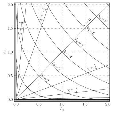
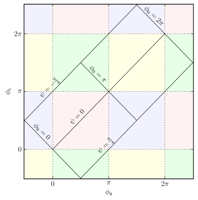
Figure 2: Correspondence between $\{A_{\textsc{r}},\phi_{\textsc{r}}\}$ and $\{A_{\textsc{l}},\phi_{\textsc{l}}\}$, which act as polar coordinates for $\{\mathcal{A}^{\breve{1}},\mathcal{A}^{\breve{2}}\}$ and $\{\mathcal{A}^{\breve{3}},\mathcal{A}^{\breve{4}}\}$, respectively, and the physical amplitude parameters $\{h_{0},\chi\mathbin{=}\cos\iota,\psi,\phi_{0}\}$. At left are lines of constant $h_{0}\in[0,\infty)$ and $\chi\in[-1,1]$, drawn in first quadrant of the $\{A_{\textsc{r}},A_{\textsc{l}}\}$ plane. (The grey shaded region, where $A_{\textsc{r}}<0$ and/or $A_{\textsc{l}}<0$, represents unphysical coordinate values.) The positive $A_{\textsc{r}}$ axis, where $A_{\textsc{l}}=0$, corresponds to $\chi=1$, where the GW signal is right circularly polarized. The positive $A_{\textsc{l}}$ axis, where $A_{\textsc{r}}=0$, corresponds to $\chi=-1$, where the GW signal is left circularly polarized. At right, the principal region of polarization $\psi\in(-\pi/4,\pi/4]$ and phase $\phi_{0}\in[0,2\pi)$ is shown in the $\{\phi_{\textsc{r}},\phi_{\textsc{l}}\}$ plane; $\phi_{\textsc{r}}$ and $\phi_{\textsc{l}}$ are each periodically identified, with period $2\pi$. Note that since the transformation $\{\psi,\phi_{0}\}\rightarrow\{\psi+\pi/2,\phi_{0}+\pi\}$ leaves the waveform unchanged, the edge $\psi=-\pi/4$, $\phi_{0}\in[0,\pi)$ is actually identified with $\psi=\pi/4$, $\phi_{0}\in[\pi,2\pi)$, while $\psi=-\pi/4$, $\phi_{0}\in[\pi,2\pi)$ is identified with $\psi=\pi/4$, $\phi_{0}\in[0,\pi)$. These periodic identifications show that the principal $\{\psi,\phi_{0}\}$ region is equivalent to the region $\phi_{\textsc{r}}\in[0,2\pi)$, $\phi_{\textsc{l}}\in[0,2\pi)$.

It is also instructive to invert (37) and write the physical coordinates $h_{0}$ and $\chi$ in terms of $A_{\textsc{r}}$ and $A_{\textsc{l}}$:

$$h_{0}=\left(\sqrt{A_{\textsc{r}}}+\sqrt{A_{\textsc{l}}}\right)^{2}\quad\hbox{and}\quad\chi=\frac{\sqrt{A_{\textsc{r}}}-\sqrt{A_{\textsc{l}}}}{\sqrt{A_{\textsc{r}}}+\sqrt{A_{\textsc{l}}}}\ ,$$ (40)

which can be related to the CPF coordinates $\{\mathcal{A}^{\breve{\mu}}\}$ by

$$A_{\textsc{r}}=\sqrt{(\mathcal{A}^{\breve{1}})^{2}+(\mathcal{A}^{\breve{2}})^{2}}\quad\hbox{and}\quad A_{\textsc{l}}=\sqrt{(\mathcal{A}^{\breve{3}})^{2}+(\mathcal{A}^{\breve{4}})^{2}}\ .$$ (41)

III.3.3 Root-radius Coordinates

Finally, it is sometimes useful to define so-called root-radius coordinates

$$r_{\textsc{r}}=A_{\textsc{r}}^{1/4} =h_{0}^{1/4}\sqrt{\frac{1+\chi}{2}}$$ (42a)

$$r_{\textsc{l}}=A_{\textsc{l}}^{1/4} =h_{0}^{1/4}\sqrt{\frac{1-\chi}{2}}$$ (42b)

with corresponding Cartesian coordinates

$$x_{\textsc{r}}=r_{\textsc{r}}\cos\phi_{\textsc{r}}\qquad \hbox{and}\qquad y_{\textsc{r}}=r_{\textsc{r}}\sin\phi_{\textsc{r}}$$ (43a)

$$x_{\textsc{l}}=r_{\textsc{l}}\cos\phi_{\textsc{l}}\qquad \hbox{and}\qquad y_{\textsc{l}}=r_{\textsc{l}}\sin\phi_{\textsc{l}}$$ (43b)

The relationship of these coordinates to the CPF coordinate system is

$$\mathcal{A}^{\breve{1}}=r_{\textsc{r}}^{3}\,x_{\textsc{r}}\qquad \hbox{and}\qquad\mathcal{A}^{\breve{2}}=r_{\textsc{r}}^{3}\,y_{\textsc{r}}$$ (44a)

$$\mathcal{A}^{\breve{3}}=r_{\textsc{l}}^{3}\,x_{\textsc{l}}\qquad \hbox{and}\qquad\mathcal{A}^{\breve{4}}=r_{\textsc{l}}^{3}\,y_{\textsc{l}}\ ,$$ (44b)

and the physical parameters can be written

$$h_{0}=(r_{\textsc{r}}^{2}+r_{\textsc{l}}^{2})^{2}\qquad\hbox{and}\qquad\chi=\frac{r_{\textsc{r}}^{2}-r_{\textsc{l}}^{2}}{r_{\textsc{r}}^{2}+r_{\textsc{l}}^{2}}\ .$$ (45)

IV Applications of the New Coordinates

IV.1 Calculation of the Jacobian Between Physical and JKS Coordinates

We can obtain the Jacobian determinant for the transformation between the physical amplitude parameters $\{h_{0},\chi\mathbin{=}\cos\iota,\psi,\phi_{0}\}$ and the JKS coordinates $\{\mathcal{A}^{1},\mathcal{A}^{2},\mathcal{A}^{3},\mathcal{A}^{4}\}$ by treating the transformation as a sequence of transformations in which the coordinates are being transformed in pairs.

First, we invert (29) to obtain

$$\mathcal{A}^{1} =\mathcal{A}^{\breve{1}}+\mathcal{A}^{\breve{3}}$$ (46a)

$$\mathcal{A}^{2} =\mathcal{A}^{\breve{2}}-\mathcal{A}^{\breve{4}}$$ (46b)

$$\mathcal{A}^{3} =-\mathcal{A}^{\breve{2}}-\mathcal{A}^{\breve{4}}$$ (46c)

$$\mathcal{A}^{4} =\mathcal{A}^{\breve{1}}-\mathcal{A}^{\breve{3}}\ ,$$ (46d)

which produces the Jacobian determinants

$$d\mathcal{A}^{1}\,d\mathcal{A}^{4}=2\,d\mathcal{A}^{\breve{1}}\,d\mathcal{A}^{\breve{3}}\quad\hbox{and}\quad d\mathcal{A}^{2}\,d\mathcal{A}^{3}=2\,d\mathcal{A}^{\breve{2}}\,d\mathcal{A}^{\breve{4}}\ .$$ (47)

Next, since (36) define $\{A_{\textsc{r}},\phi_{\textsc{r}}\}$ as the polar coordinates corresponding to the Cartesian coordinates $\{\mathcal{A}^{\breve{1}},\mathcal{A}^{\breve{2}}\}$, and likewise for $\{A_{\textsc{l}},\phi_{\textsc{l}}\}$ and $\{\mathcal{A}^{\breve{3}},\mathcal{A}^{\breve{4}}\}$, the relevant Jacobian determinants are

$$d\mathcal{A}^{\breve{1}}\,d\mathcal{A}^{\breve{2}}=A_{\textsc{r}}\,dA_{\textsc{r}}\,d\phi_{\textsc{r}}\quad\hbox{and}\quad d\mathcal{A}^{\breve{3}}\,d\mathcal{A}^{\breve{4}}=A_{\textsc{l}}\,dA_{\textsc{l}}\,d\phi_{\textsc{l}}\ .$$ (48)

Finally, the identifications (37) lead to the Jacobian matrices

$$\begin{pmatrix}dA_{\textsc{r}}\\ dA_{\textsc{l}}\end{pmatrix}=\begin{pmatrix}\left(\frac{1+\chi}{2}\right)^{2}&h_{0}\frac{1+\chi}{2}\\ \left(\frac{1-\chi}{2}\right)^{2}&-h_{0}\frac{1-\chi}{2}\end{pmatrix}\begin{pmatrix}dh_{0}\\ d\chi\end{pmatrix}$$ (49)

and

$$\begin{pmatrix}d\phi_{\textsc{r}}\\ d\phi_{\textsc{l}}\end{pmatrix}=\begin{pmatrix}2&1\\ -2&1\end{pmatrix}\begin{pmatrix}d\psi\\ d\phi_{0}\end{pmatrix}\ ,$$ (50)

whose determinants tell us

$$dA_{\textsc{r}}\,dA_{\textsc{l}}=h_{0}\frac{1-\chi^{2}}{4}\,dh_{0}\,d\chi\quad\hbox{and}\quad d\phi_{\textsc{r}}\,d\phi_{\textsc{l}}=4\,d\psi\,d\phi_{0}\ .$$ (51)

To combine the effects of these three transformations, note from (37) that

$$A_{\textsc{r}}A_{\textsc{l}}=\left(h_{0}\frac{1-\chi^{2}}{4}\right)^{2}$$ (52)

and thus

$$d\mathcal{A}^{1}\,d\mathcal{A}^{2}\,d\mathcal{A}^{3}\,d\mathcal{A}^{4}=4\,d\mathcal{A}^{\breve{1}}\,d\mathcal{A}^{\breve{2}}\,d\mathcal{A}^{\breve{3}}\,d\mathcal{A}^{\breve{4}}\\ =4A_{\textsc{r}}A_{\textsc{l}}\,dA_{\textsc{r}}\,dA_{\textsc{l}}\,d\phi_{\textsc{r}}\,d\phi_{\textsc{l}}\\ =16\left(h_{0}\frac{1-\chi^{2}}{4}\right)^{3}\,dh_{0}\,d\chi\,d\psi\,d\phi_{0}$$ (53)

which is the same as the form (27) presented in Prix09:_Bstat .

Note that, using (52) we can rewrite (53) as

$$dh_{0}\,d\chi\,d\psi\,d\phi_{0}=\frac{dA_{\textsc{r}}\,dA_{\textsc{l}}\,d\phi_{\textsc{r}}\,d\phi_{\textsc{l}}}{4\sqrt{A_{\textsc{r}}A_{\textsc{l}}}}\\ =\frac{d\mathcal{A}^{\breve{1}}\,d\mathcal{A}^{\breve{2}}\,d\mathcal{A}^{\breve{3}}\,d\mathcal{A}^{\breve{4}}}{4\bigl{[}(\mathcal{A}^{\breve{1}})^{2}+(\mathcal{A}^{\breve{2}})^{2}\bigr{]}^{3/4}\bigr{[}(\mathcal{A}^{\breve{3}})^{2}+(\mathcal{A}^{\breve{4}})^{2}\bigr{]}^{3/4}}\ .$$ (54)

If we recall the root-radius coordinates defined so that $r_{\textsc{r}}^{2}=A_{\textsc{r}}^{1/2}$ and $r_{\textsc{l}}^{2}=A_{\textsc{l}}^{1/2}$, we have

$$\frac{dA_{\textsc{r}}}{2\sqrt{A_{\textsc{r}}}}=2r_{\textsc{r}}\,dr_{\textsc{r}}\qquad\hbox{and}\qquad\frac{dA_{\textsc{l}}}{2\sqrt{A_{\textsc{l}}}}=2r_{\textsc{l}}\,dr_{\textsc{l}}\ ,$$ (55)

so that

$$\begin{split}dh_{0}\,d\chi\,d\psi\,d\phi_{0}&=4\,r_{\textsc{r}}\,dr_{\textsc{r}}\,d\phi_{\textsc{r}}\,r_{\textsc{l}}\,dr_{\textsc{l}}\,d\phi_{\textsc{l}}\\ &=4\,dx_{\textsc{r}}\,dy_{\textsc{r}}\,dx_{\textsc{l}}\,dy_{\textsc{l}}\ ,\end{split}$$ (56)

i.e., the natural measure in physical coordinates is, up to a constant, just the usual Lebesgue measure on a Cartesian space.

IV.2 Nature of the Coordinate Singularities for Circular Polarization

The volume element (53) has singularities in terms of the physical coordinates for circular polarization, i.e., $\chi=\pm 1$, because the Jacobian

$$\begin{split}\mathcal{J}&=2\left(h_{0}\frac{1-\chi^{2}}{2}\right)^{3}=2\left(A_{+}^{2}-A_{\times}^{2}\right)^{3/2}=16\,(A_{\textsc{r}}A_{\textsc{l}})^{3/2}\\ &=16\,\Bigl{\{}\Bigl{[}(\mathcal{A}^{\breve{1}})^{2}+(\mathcal{A}^{\breve{2}})^{2}\Bigr{]}\Bigr{[}(\mathcal{A}^{\breve{3}})^{2}+(\mathcal{A}^{\breve{4}})^{2}\Bigr{]}\Bigr{\}}^{3/4}\end{split}$$ (57)

vanishes there.

IV.2.1 Right Circular Polarization ($\chi=1$, i.e., $\iota=0$)

When $\chi=1$, so that $A_{\times}=A_{+}$, the polar amplitude coordinates become $A_{\textsc{r}}=h_{0}$ and $A_{\textsc{l}}=0$, so the combination $A_{\textsc{r}}A_{\textsc{l}}$ vanishes, and the amplitude parameters become

$$\mathcal{A}^{1}=\mathcal{A}^{4}=\mathcal{A}^{\breve{1}} =h_{0}\cos(\phi_{0}+2\psi)$$ (58a)

$$\mathcal{A}^{2}=-\mathcal{A}^{3}=\mathcal{A}^{\breve{2}} =h_{0}\sin(\phi_{0}+2\psi)$$ (58b)

$$\mathcal{A}^{\breve{3}}=\mathcal{A}^{\breve{4}} =0$$ (58c)

The waveform (1) is completely described by the amplitude $h_{0}$ and the phase $\phi_{\textsc{r}}=\phi_{0}+2\psi$, exhibiting the well-known degeneracy between $\psi$ and $\phi_{0}$ for circular polarization.

IV.2.2 Left Circular Polarization ($\chi=-1$, i.e., $\iota=\pi$)

When $\chi=-1$, so that $A_{\times}=-A_{+}$, the polar amplitude coordinates become $A_{\textsc{r}}=0$ and $A_{\textsc{l}}=h_{0}$, so the combination $A_{\textsc{r}}A_{\textsc{l}}$ vanishes, and the amplitude parameters become

$$\mathcal{A}^{\breve{1}}=\mathcal{A}^{\breve{2}} =0$$ (59a)

$$\mathcal{A}^{1}=-\mathcal{A}^{4}=\mathcal{A}^{\breve{3}} =h_{0}\cos(\phi_{0}-2\psi)$$ (59b)

$$-\mathcal{A}^{2}=-\mathcal{A}^{3}=\mathcal{A}^{\breve{4}} =h_{0}\sin(\phi_{0}-2\psi)$$ (59c)

The waveform (1) is completely described by the amplitude $h_{0}$ and the phase $\phi_{\textsc{l}}=\phi_{0}-2\psi$, exhibiting the well-known degeneracy between $\psi$ and $\phi_{0}$ for circular polarization.

V Integration techniques for the $\mathcal{B}$-statistic targeted search method

Prix and Krishnan Prix09:_Bstat consider the case of a targeted search, where the signal hypothesis $\mathcal{H}_{s}$ has known phase-evolution parameters $\{\alpha,\delta,f_{0},f_{1},\ldots\}$ but unknown amplitude parameters, obeying some prior probability distribution $\text{pdf}(\mathcal{A}|\mathcal{H}_{s})$. Given some observed data ${x}$, they calculate the Bayes factor

$$\begin{split}\mathcal{B}({x})&=\frac{\text{pdf}({x}|\mathcal{H}_{s})}{\text{pdf}({x}|\mathcal{H}_{n})}=\frac{\int\text{pdf}({x}|\mathcal{H}_{s},\mathcal{A})\,\text{pdf}(\mathcal{A}|\mathcal{H}_{s})\,d^{4}\!\mathcal{A}}{\text{pdf}({x}|\mathcal{H}_{n})}\\ &=\int e^{\Lambda(\mathcal{A};{x})}\,\text{pdf}(\mathcal{A}|\mathcal{H}_{s})\,d^{4}\!\mathcal{A}\ ,\end{split}$$ (60)

which they call the $\mathcal{B}$-statistic, in contrast with the $\mathcal{F}$-statistic, which is the maximum log-likelihood ratio

$$\mathcal{F}({x})=\max_{\mathcal{A}}\ln\frac{\text{pdf}({x}|\mathcal{H}_{s},\mathcal{A})}{\text{pdf}({x}|\mathcal{H}_{n})}=\max_{\mathcal{A}}\Lambda(\mathcal{A};{x})\ .$$ (61)

V.1 Form of the Log-Likelihood Ratio

The log-likelihood ratio can be written in the form krolak04:_optim_lisa ; WhelanPrix08:_MLDC1B

$$\Lambda(\{\mathcal{A}^{\mu}\};{x})=\mathcal{A}^{\mu}x_{\mu}-\frac{1}{2}\mathcal{A}^{\mu}\mathcal{M}_{\mu\nu}\mathcal{A}^{\nu}$$ (62)

where we defined

$$x_{\mu}\equiv\left({x}|{h}_{\mu}\right)\ ,\quad\text{and}\quad\mathcal{M}_{\mu\nu}\equiv\left({h}_{\mu}|{h}_{\nu}\right)\ ,$$ (63)

in terms of the standard scalar product $\left(\cdot|\cdot\right)$ defined in (128), the strain data $x$ and the four scalar basis waveforms $h_{\mu}$, which are the detector’s response to the four GW tensor functions ${\mathchoice{\mathord{\hbox to0.0pt{\hbox to8.79988pt{\hss$\displaystyle h$\hss}\hss}\raise 7.98605pt\hbox to8.79988pt{\hss\hbox{$\scriptstyle\leftrightarrow$}\hss}}}{\mathord{\hbox to0.0pt{\hbox to8.79988pt{\hss$\textstyle h$\hss}\hss}\raise 7.98605pt\hbox to8.79988pt{\hss\hbox{$\scriptstyle\leftrightarrow$}\hss}}}{\mathord{\hbox to0.0pt{\hbox to6.99988pt{\hss$\scriptstyle h$\hss}\hss}\raise 5.59023pt\hbox to6.99988pt{\hss\hbox{$\scriptscriptstyle\leftrightarrow$}\hss}}}{\mathord{\hbox to0.0pt{\hbox to6.99988pt{\hss$\scriptscriptstyle h$\hss}\hss}\raise 3.99301pt\hbox to6.99988pt{\hss\hbox{$\scriptscriptstyle\leftrightarrow$}\hss}}}}\mathord{\hbox{}}_{\mu}$ according to (9). As shown in appendix A, the matrix $\{\mathcal{M}_{\mu\nu}\}$ is explicitly found to have the form

$$\{\mathcal{M}_{\mu\nu}\}=\begin{pmatrix}A&C&0&E\\ C&B&-E&0\\ 0&-E&A&C\\ E&0&C&B\end{pmatrix}\ .$$ (64)

In the long-wavelength limit, $E=0$; it is non-zero only in the regime where the finite size of the detector is important, and the simple response tensor (13) is replaced by a complex frequency-dependent expression.

Since the new amplitude coordinates $\{\mathcal{A}^{\breve{\mu}}\}$ are linear combinations of the $\{\mathcal{A}^{\mu}\}$, we can also write the log-likelihood ratio as a quadratic in those coordinates:

$$\Lambda(\{\mathcal{A}^{\breve{\mu}}\};{x})=\mathcal{A}^{\breve{\mu}}x_{\breve{\mu}}-\frac{1}{2}\mathcal{A}^{\breve{\mu}}\mathcal{M}_{\breve{\mu}\breve{\nu}}\mathcal{A}^{\breve{\nu}}\ ,$$ (65)

with

$$x_{\breve{\mu}}=\left(x|h_{\breve{\mu}}\right)\ ,\quad\text{and}\quad\mathcal{M}_{\breve{\mu}\breve{\nu}}=\left(h_{\breve{\mu}}|h_{\breve{\nu}}\right)\ ,$$ (66)

in analogy to (63), and the transformed matrix is found to have the form

$$\{\mathcal{M}_{\breve{\mu}\breve{\nu}}\}=\begin{pmatrix}I&0&L&-K\\ 0&I&K&L\\ L&K&J&0\\ -K&L&0&J\end{pmatrix}\ ,$$ (67)

with the explicit matrix elements given in appendix A, and in the long-wavelength limit we have $I=J$.

In terms of the data vector $\{x_{\breve{\mu}}\}$ (whose explicit form is given in appendix A), the linear part of the log-likelihood ratio is

$$\mathcal{A}^{\breve{\mu}}x_{\breve{\mu}}=A_{\textsc{r}}(x_{\breve{1}}\cos\phi_{\textsc{r}}+x_{\breve{2}}\sin\phi_{\textsc{r}})+A_{\textsc{l}}(x_{\breve{3}}\cos\phi_{\textsc{l}}+x_{\breve{4}}\sin\phi_{\textsc{l}})\ .$$ (68)

The quadratic part of the log-likelihood can be written in the $\{\mathcal{A}^{\breve{\mu}}\}$ coordinates as

$$\begin{split}\mathcal{A}^{\breve{\mu}}\mathcal{M}_{\breve{\mu}\breve{\nu}}&\mathcal{A}^{\breve{\nu}}=I[(\mathcal{A}^{\breve{1}})^{2}+(\mathcal{A}^{\breve{2}})^{2}]+J[(\mathcal{A}^{\breve{3}})^{2}+(\mathcal{A}^{\breve{4}})^{2}]\\ &+2K[-\mathcal{A}^{\breve{1}}\mathcal{A}^{\breve{4}}+\mathcal{A}^{\breve{2}}\mathcal{A}^{\breve{3}}]+2L[\mathcal{A}^{\breve{1}}\mathcal{A}^{\breve{3}}+\mathcal{A}^{\breve{2}}\mathcal{A}^{\breve{4}}]\\ =\ &IA_{\textsc{r}}^{2}+JA_{\textsc{l}}^{2}\\ &+2A_{\textsc{r}}A_{\textsc{l}}\left[K\sin(\phi_{\textsc{r}}-\phi_{\textsc{l}})+L\cos(\phi_{\textsc{r}}-\phi_{\textsc{l}})\right]\ .\end{split}$$ (69)

Note that this depends upon the angular coordinates only in the combination $\phi_{\textsc{r}}-\phi_{\textsc{l}}=4\psi$, and is independent of $\phi_{\textsc{r}}+\phi_{\textsc{l}}=2\phi_{0}$.

Because the amplitude parameters $\{\mathcal{A}^{\breve{\mu}}\}$ which maximize the log-likelihood ratio $\Lambda(\{\mathcal{A}^{\breve{\mu}}\};{x})$ are given by

$$\widehat{\mathcal{A}}^{\breve{\mu}}({x})=\mathcal{M}^{\breve{\mu}\breve{\nu}}x_{\breve{\nu}}\ ,$$ (70)

where $\{\mathcal{M}^{\breve{\mu}\breve{\nu}}\}$ is the matrix inverse of $\{\mathcal{M}_{\breve{\mu}\breve{\nu}}\}$, and the maximum of the log-likelihood ratio is the $\mathcal{F}$-statistic

$$\mathcal{F}({x})=\frac{1}{2}x_{\breve{\mu}}\mathcal{M}^{\breve{\mu}\breve{\nu}}x_{\breve{\nu}}=\frac{1}{2}\widehat{\mathcal{A}}^{\breve{\mu}}({x})\mathcal{M}_{\breve{\mu}\breve{\nu}}\widehat{\mathcal{A}}^{\breve{\nu}}({x})\ ,$$ (71)

it is convenient to write the log-likelihood ratio as

$$\Lambda(\{\mathcal{A}^{\breve{\mu}}\};{x})=\mathcal{F}({x})-\frac{1}{2}[\mathcal{A}^{\breve{\mu}}-\widehat{\mathcal{A}}^{\breve{\mu}}({x})]\mathcal{M}_{\breve{\mu}\breve{\nu}}[\mathcal{A}^{\breve{\nu}}-\widehat{\mathcal{A}}^{\breve{\nu}}({x})]\ .$$ (72)

V.2 Integration in CPF coordinates

Since the log-likelihood ratio $\Lambda(\mathcal{A};{x})$ (72) is quadratic in $\{\mathcal{A}^{\breve{\mu}}\}$ (just as it is in $\{\mathcal{A}^{\mu}\}$) we can do the Gaussian integral, for the case of the unphysical $\mathcal{F}$-statistic prior (26), as shown in Prix09:_Bstat :

$$\begin{split}\mathcal{B}({x})&=\int e^{\Lambda(\mathcal{A};{x})}\,\text{pdf}(\mathcal{A}|\mathcal{H}_{s})\,d^{4}\!\mathcal{A}\\ &\propto\int e^{\mathcal{A}^{\breve{\mu}}x_{\breve{\mu}}-\frac{1}{2}\mathcal{A}^{\breve{\mu}}\mathcal{M}_{\breve{\mu}\breve{\nu}}\mathcal{A}^{\breve{\nu}}}\,d\mathcal{A}^{\breve{1}}\,d\mathcal{A}^{\breve{2}}\,d\mathcal{A}^{\breve{3}}\,d\mathcal{A}^{\breve{4}}\\ &=e^{\mathcal{F}({x})}\int e^{-\frac{1}{2}\Delta\mathcal{A}^{\breve{\mu}}\mathcal{M}_{\breve{\mu}\breve{\nu}}\Delta\mathcal{A}^{\breve{\nu}}}\,d\mathcal{A}^{\breve{1}}\,d\mathcal{A}^{\breve{2}}\,d\mathcal{A}^{\breve{3}}\,d\mathcal{A}^{\breve{4}}\\ &\propto e^{\mathcal{F}({x})}\ .\end{split}$$ (73)

If, however, an isotropic prior(18) is used, so that

$$\text{pdf}(\{\mathcal{A}^{\breve{\mu}}\}|\mathcal{H}_{s})=\text{pdf}(\mathcal{A}^{\breve{1}},\mathcal{A}^{\breve{2}},\mathcal{A}^{\breve{3}},\mathcal{A}^{\breve{4}}|\mathcal{H}_{s})\\ =\frac{4}{\mathcal{J}}\text{pdf}(h_{0},\chi,\psi,\phi_{0}|\mathcal{H}_{s})=\frac{2}{\pi^{2}}\frac{\text{pdf}(h_{0}|\mathcal{H}_{s})}{\mathcal{J}}\ ,$$ (74)

where $\mathcal{J}$ is the Jacobian determinant specified in (57). Then if we define

$$\alpha(\mathcal{A})=\ln\frac{\text{pdf}(h_{0}|\mathcal{H}_{s})}{\mathcal{J}}\ ,$$ (75)

the $\mathcal{B}$-statistic integral can be written as

$$\mathcal{B}({x})\propto e^{\mathcal{F}({x})}\int e^{-\frac{1}{2}\Delta\mathcal{A}^{\breve{\mu}}\mathcal{M}_{\breve{\mu}\breve{\nu}}\Delta\mathcal{A}^{\breve{\nu}}+\alpha(\mathcal{A})}\,d\mathcal{A}^{\breve{1}}\,d\mathcal{A}^{\breve{2}}\,d\mathcal{A}^{\breve{3}}\,d\mathcal{A}^{\breve{4}}\ .$$ (76)

One possible approach would be to Taylor expand $\alpha(\mathcal{A})$ about the maximum-likelihood point $\widehat{\mathcal{A}}$,

$$\alpha(\mathcal{A})=\widehat{\alpha}+\widehat{\alpha}_{\breve{\mu}}\Delta\mathcal{A}^{\breve{\mu}}+\frac{1}{2}\widehat{\alpha}_{\breve{\mu}\breve{\nu}}\Delta\mathcal{A}^{\breve{\mu}}\Delta\mathcal{A}^{\breve{\nu}}+\mathcal{O}([\Delta\mathcal{A}]^{3})\ ,$$ (77)

where we have defined the expansion coefficients

$$\widehat{\alpha} =\alpha(\widehat{\mathcal{A}})$$ (78a)

$$\widehat{\alpha}_{\breve{\mu}} =\left.\frac{\partial\alpha}{\partial\mathcal{A}^{\breve{\mu}}}\right\rvert_{\mathcal{A}=\widehat{\mathcal{A}}}$$ (78b)

$$\widehat{\alpha}_{\breve{\mu}\breve{\nu}} =\left.\frac{\partial^{2}\alpha}{\partial\mathcal{A}^{\breve{\mu}}\partial\mathcal{A}^{\breve{\nu}}}\right\rvert_{\mathcal{A}=\widehat{\mathcal{A}}}\,.$$ (78c)

(This was the method used in Cohen et al. 2010CQGra..27r5012C for approximating the analog of the $\mathcal{B}$-statistic for the case of GW bursts from cosmic strings.) We could then approximate the integral as Gaussian, obtaining the result

$$\begin{split}\mathcal{B}({x})\propto&\left(\det\{\mathcal{N}_{\breve{\mu}\breve{\nu}}({x})\}\right)^{-1/2}\\ &\times\exp\left(\mathcal{F}({x})+\widehat{\alpha}({x})\ +\frac{1}{2}\widehat{\alpha}_{\breve{\mu}}({x})\mathcal{N}^{\breve{\mu}\breve{\nu}}({x})\widehat{\alpha}_{\breve{\nu}}({x})\right)\ ,\end{split}$$ (79)

where we have defined the matrix

$$\mathcal{N}_{\breve{\mu}\breve{\nu}}({x})=\mathcal{M}_{\breve{\mu}\breve{\nu}}-\widehat{\alpha}_{\breve{\mu}\breve{\nu}}({x})$$ (80)

and its inverse $\mathcal{N}^{\breve{\mu}\breve{\nu}}$ (so that $\mathcal{N}^{\breve{\mu}\breve{\nu}}\mathcal{N}_{\breve{\nu}\breve{\sigma}}=\delta_{\sigma}^{\mu}$). However, this approximation can only be valid if the matrix $\mathcal{N}^{\breve{\mu}\breve{\nu}}$ is positive definite, so that the point $\mathcal{A}^{\breve{\mu}}=\widehat{\mathcal{A}}^{\breve{\mu}}+\mathcal{N}^{\breve{\mu}\breve{\nu}}\widehat{\alpha}_{\breve{\nu}}$ is a maximum of the integrand in (76). We will show that that is not in general true by calculating the explicit form of $\widehat{\alpha}_{\breve{\mu}\breve{\nu}}$.

We limit attention to the simple case of a uniform prior on $h_{0}$, $\text{pdf}(h_{0}|\mathcal{H}_{s})=\text{const}$. In that case,

$$\alpha(\mathcal{A})=-\ln\mathcal{J}+\text{const}=-\frac{3}{2}\ln(A_{\textsc{r}}A_{\textsc{l}})+\text{const}\\ =-\frac{3}{4}\ln\left([\mathcal{A}^{\breve{1}}]^{2}+[\mathcal{A}^{\breve{2}}]^{2}\right)-\frac{3}{4}\ln\left([\mathcal{A}^{\breve{3}}]^{2}+[\mathcal{A}^{\breve{4}}]^{2}\right)+\text{const}\ ,$$ (81)

and we can calculate the unique non-vanishing derivatives as

$$\frac{\partial\alpha}{\partial\mathcal{A}^{\breve{1}}}=-\frac{3}{2}\frac{\mathcal{A}^{\breve{1}}}{[\mathcal{A}^{\breve{1}}]^{2}+[\mathcal{A}^{\breve{2}}]^{2}}$$ (82)

and

$$\frac{\partial^{2}\alpha}{(\partial\mathcal{A}^{\breve{1}})^{2}} =-\frac{3}{2}\frac{[\mathcal{A}^{\breve{2}}]^{2}-[\mathcal{A}^{\breve{1}}]^{2}}{([\mathcal{A}^{\breve{1}}]^{2}+[\mathcal{A}^{\breve{2}}]^{2})^{2}}=\frac{3}{2}\frac{\cos 2\phi_{\textsc{r}}}{A_{\textsc{r}}^{2}}$$ (83a)

$$\frac{\partial^{2}\alpha}{\partial\mathcal{A}^{\breve{1}}\partial\mathcal{A}^{\breve{2}}} =\frac{3}{2}\frac{2\mathcal{A}^{\breve{1}}\mathcal{A}^{\breve{2}}}{([\mathcal{A}^{\breve{1}}]^{2}+[\mathcal{A}^{\breve{2}}]^{2})^{2}}=\frac{3}{2}\frac{\sin 2\phi_{\textsc{r}}}{A_{\textsc{r}}^{2}}\ ,$$ (83b)

with the derivatives with respect to the other $\{\mathcal{A}^{\breve{\mu}}\}$ following by inspection. The resulting matrix is

$$\widehat{\alpha}_{\breve{\mu}\breve{\nu}}=\frac{3}{2}\begin{pmatrix}\frac{\cos 2\widehat{\phi}_{\textsc{r}}}{\widehat{A}_{\textsc{r}}^{2}}&\frac{\sin 2\widehat{\phi}_{\textsc{r}}}{\widehat{A}_{\textsc{r}}^{2}}&0&0\\ \frac{\sin 2\widehat{\phi}_{\textsc{r}}}{\widehat{A}_{\textsc{r}}^{2}}&-\frac{\cos 2\widehat{\phi}_{\textsc{r}}}{\widehat{A}_{\textsc{r}}^{2}}&0&0\\ 0&0&\frac{\cos 2\widehat{\phi}_{\textsc{l}}}{\widehat{A}_{\textsc{l}}^{2}}&\frac{\sin 2\widehat{\phi}_{\textsc{l}}}{\widehat{A}_{\textsc{l}}^{2}}\\ 0&0&\frac{\sin 2\widehat{\phi}_{\textsc{l}}}{\widehat{A}_{\textsc{l}}^{2}}&-\frac{\cos 2\widehat{\phi}_{\textsc{l}}}{\widehat{A}_{\textsc{l}}^{2}}\end{pmatrix}\ .$$ (84)

Now, if the data happen to be such that the maximum likelihood estimates of the amplitude parameters $\widehat{\mathcal{A}}$ correspond to right- or left-circular polarization, then the parameter $\widehat{A}_{\textsc{r}}$ or $\widehat{A}_{\textsc{l}}$, respectively, will be small. Since the metric $\{\mathcal{M}_{\breve{\mu}\breve{\nu}}\}$ is determined by the observing geometry and the noise level, and not the realization of the data, it can always happen that $\widehat{A}_{\textsc{r}}$ or $\widehat{A}_{\textsc{l}}$ is small enough that two of the eigenvalues of $\mathcal{N}_{\breve{\mu}\breve{\nu}}({x})=\mathcal{M}_{\breve{\mu}\breve{\nu}}-\widehat{\alpha}_{\breve{\mu}\breve{\nu}}({x})$ will be approximately equal to the corresponding eigenvalues of $-\widehat{\alpha}_{\breve{\mu}\breve{\nu}}({x})$, which will be the eigenvalues of the matrix

$$\frac{3}{2\widehat{A}_{\textsc{r}}^{2}}\begin{pmatrix}-\cos 2\widehat{\phi}_{\textsc{r}}&-\sin 2\widehat{\phi}_{\textsc{r}}\\ -\sin 2\widehat{\phi}_{\textsc{r}}&\cos 2\widehat{\phi}_{\textsc{r}}\end{pmatrix}\ ,$$ (85)

which are $\pm\frac{3}{2A_{\textsc{r}}^{2}}$ (or the corresponding expression involving $A_{\textsc{l}}$, in the case of left circular polarization). Since these two eigenvalues have opposite signs, $\{\mathcal{N}_{\breve{\mu}\breve{\nu}}\}$ is not a positive definite matrix, the point $\mathcal{A}^{\breve{\mu}}=\widehat{\mathcal{A}}^{\breve{\mu}}+\mathcal{N}^{\breve{\mu}\breve{\nu}}\widehat{\alpha}_{\breve{\nu}}$ is a saddle point rather than a maximum, and the Gaussian approximation for the integral (76) fails.

One issue with this approach is that the maximum likelihood point is a stationary point of $\Lambda(\mathcal{A};{x})$ rather than $\Lambda(\mathcal{A};{x})+\alpha(\mathcal{A})$, and we should consider expanding about the maximum of $\Lambda(\mathcal{A};{x})+\alpha(\mathcal{A})$. In fact, $\Lambda(\mathcal{A};{x})+\alpha(\mathcal{A})$ has no global maximum, as examination of (81) shows that $\alpha(\mathcal{A})\rightarrow+\infty$ as $A_{\textsc{r}}$ or $A_{\textsc{l}}$ goes to zero. The best we can hope for is a local maximum when

$$\frac{\partial}{\partial\mathcal{A}^{\breve{\mu}}}\left[\Lambda(\mathcal{A};{x})+\alpha(\mathcal{A})\right]=x_{\breve{\mu}}-\mathcal{M}_{\breve{\mu}\breve{\nu}}\mathcal{A}^{\breve{\nu}}+\alpha_{\breve{\mu}}(\mathcal{A})=0\ .$$ (86)

This local maximum can fail to exist even when the matrix $\{\mathcal{N}_{\breve{\mu}\breve{\nu}}\}$ is positive definite, and in any event, the Gaussian integral would only approximate the area under the local maximum, not the contribution from the integrable singularity at $A_{\textsc{r}}=0$ and $A_{\textsc{l}}=0$. This is examined in further detail in section VI.3.

V.3 Integration in root-radius coordinates

As we’ve seen in section V.2, while the log-likelihood ratio is quadratic in CPF (or JKS) coordinates, the integrand of the $\mathcal{B}$-statistic integral arising from an isotropic prior (18) contains a coordinate singularity which prevents the integrand from being approximated by a Gaussian. If we focus attention on the constant-$h_{0}$ prior

$$\text{pdf}(h_{0},\chi,\psi,\phi_{0}|\mathcal{H}_{s})=\text{const}\ ,$$ (87)

the measure of the integral will be constant not only in physical coordinates $\{h_{0},\chi,\psi,\phi_{0}\}$ but also in the root-radius Cartesian coordinates $\{x_{\textsc{r}},y_{\textsc{r}},x_{\textsc{l}},y_{\textsc{l}}\}$ defined in section III.3.3 [see (56)]. The integral will not be a Gaussian, since the log-likelihood ratio will no longer be quadratic in these coordinates, but it will remain non-singular and have a single maximum at the point $\mathcal{A}=\widehat{\mathcal{A}}$. Thus we can write the integral as

$$\mathcal{B}({x})\propto\int_{-\infty}^{\infty}\int_{-\infty}^{\infty}\int_{-\infty}^{\infty}\int_{-\infty}^{\infty}e^{\Lambda(\mathcal{A};{x})}\,dx_{\textsc{r}}\,dy_{\textsc{r}}\,dx_{\textsc{l}}\,dy_{\textsc{l}}$$ (88)

and attempt to Taylor expand the log of the integrand, $\Lambda(\mathcal{A};{x})$, about its maximum. Writing

$$\{\mathcal{A}^{\alpha}\}=\{x_{\textsc{r}},y_{\textsc{r}},x_{\textsc{l}},y_{\textsc{l}}\}\ ,$$ (89)

the expansion is

$$\begin{split}\Lambda(\mathcal{A};{x})=&\Lambda(\widehat{\mathcal{A}};{x})+\left.\frac{\partial\Lambda}{\partial\mathcal{A}^{\alpha}}\right\rvert_{\mathcal{A}=\widehat{A}}(\mathcal{A}^{\alpha}-\widehat{\mathcal{A}}^{\alpha})\\ &+\frac{1}{2}\left.\frac{\partial^{2}\Lambda}{\partial\mathcal{A}^{\alpha}\partial\mathcal{A}^{\beta}}\right\rvert_{\mathcal{A}=\widehat{A}}(\mathcal{A}^{\alpha}-\widehat{\mathcal{A}}^{\alpha})(\mathcal{A}^{\beta}-\widehat{\mathcal{A}}^{\beta})\\ &+\mathcal{O}([\mathcal{A}-\widehat{\mathcal{A}}]^{3})\ .\end{split}$$ (90)

Since $\widehat{\mathcal{A}}$ is the maximum-likelihood point, $\Lambda(\widehat{\mathcal{A}};{x})=\mathcal{F}({x})$ and $\left.\frac{\partial\Lambda}{\partial\mathcal{A}^{\alpha}}\right\rvert_{\mathcal{A}=\widehat{A}}=0$. If we use (72) to calculate

$$\frac{\partial^{2}\Lambda}{\partial\mathcal{A}^{\alpha}\partial\mathcal{A}^{\beta}}=\frac{\partial^{2}\mathcal{A}^{\breve{\mu}}}{\partial\mathcal{A}^{\alpha}\partial\mathcal{A}^{\beta}}\mathcal{M}_{\breve{\mu}\breve{\nu}}[\mathcal{A}^{\breve{\nu}}-\widehat{\mathcal{A}}^{\breve{\nu}}({x})]+\frac{\partial\mathcal{A}^{\breve{\mu}}}{\partial\mathcal{A}^{\alpha}}\mathcal{M}_{\breve{\mu}\breve{\nu}}\frac{\partial\mathcal{A}^{\breve{\nu}}}{\partial\mathcal{A}^{\beta}}\ ,$$ (91)

we see that

$$\left.\frac{\partial^{2}\Lambda}{\partial\mathcal{A}^{\alpha}\partial\mathcal{A}^{\beta}}\right\rvert_{\mathcal{A}=\widehat{A}}=\left.\frac{\partial\mathcal{A}^{\breve{\mu}}}{\partial\mathcal{A}^{\alpha}}\right\rvert_{\mathcal{A}=\widehat{A}}\mathcal{M}_{\breve{\mu}\breve{\nu}}\left.\frac{\partial\mathcal{A}^{\breve{\nu}}}{\partial\mathcal{A}^{\beta}}\right\rvert_{\mathcal{A}=\widehat{A}}\ .$$ (92)

Thus

$$\Lambda(\mathcal{A};{x})\\ =\mathcal{F}({x})+\frac{1}{2}\left.\frac{\partial\mathcal{A}^{\breve{\mu}}}{\partial\mathcal{A}^{\alpha}}\right\rvert_{\mathcal{A}=\widehat{A}}\mathcal{M}_{\breve{\mu}\breve{\nu}}\left.\frac{\partial\mathcal{A}^{\breve{\nu}}}{\partial\mathcal{A}^{\beta}}\right\rvert_{\mathcal{A}=\widehat{A}}(\mathcal{A}^{\alpha}-\widehat{\mathcal{A}}^{\alpha})(\mathcal{A}^{\beta}-\widehat{\mathcal{A}}^{\beta})\\ +\mathcal{O}([\mathcal{A}-\widehat{\mathcal{A}}]^{3})\ ;$$ (93)

if we keep only the quadratic piece, we get the approximate Gaussian integral

$$\begin{split}\ln\mathcal{B}({x})&\approx\mathcal{F}({x})-\frac{1}{2}\ln\det\left\{\left.\frac{\partial^{2}\Lambda}{\partial\mathcal{A}^{\alpha}\partial\mathcal{A}^{\beta}}\right\rvert_{\mathcal{A}=\widehat{A}({x})}\right\}+\text{const}\\ &\approx\mathcal{F}({x})-\ln\det\left\{\left.\frac{\partial\mathcal{A}^{\breve{\mu}}}{\partial\mathcal{A}^{\alpha}}\right\rvert_{\mathcal{A}=\widehat{A}({x})}\right\}+\text{const}\ ,\end{split}$$ (94)

where we have absorbed the term $-\frac{1}{2}\det\left\{\mathcal{M}_{\breve{\mu}\breve{\nu}}\right\}$ into the constant since it does not depend on the data.

The determinant

$$\det\left\{\frac{\partial\mathcal{A}^{\breve{\mu}}}{\partial\mathcal{A}^{\alpha}}\right\}=16(A_{\textsc{r}}A_{\textsc{l}})^{3/2}$$ (95)

has already been calculated, since it’s the Jacobian for the transformation between the coordinates $\{\mathcal{A}^{\alpha}\}=\{x_{\textsc{r}},y_{\textsc{r}},x_{\textsc{l}},y_{\textsc{l}}\}$ and $\{\mathcal{A}^{\breve{\mu}}\}=\{\mathcal{A}^{\breve{1}},\mathcal{A}^{\breve{2}},\mathcal{A}^{\breve{3}},\mathcal{A}^{\breve{4}}\}$. This means that

$$\ln\mathcal{B}({x})\approx\mathcal{F}({x})-\frac{3}{2}\ln\left(\widehat{A}_{\textsc{r}}({x})\,\widehat{A}_{\textsc{l}}({x})\right)+\text{const}\ .$$ (96)

This approximate correction factor in $\mathcal{B}({x})$ has a familiar form: it’s the Jacobian appearing in the Gaussian integral in CPF coordinates, evaluated at the maximum likelihood point. The approximation again breaks down if the maximum likelihood point is too close to circular polarization, i.e., if $\widehat{A}_{\textsc{r}}({x})$ or $\widehat{A}_{\textsc{l}}({x})$ is close to zero. It’s easy to see why this is the case: the log-likelihood-ratio $\Lambda(\mathcal{A};{x})$ has terms proportional to $(A_{\textsc{r}}-\widehat{A}_{\textsc{r}}({x}))^{2}$ and $(A_{\textsc{l}}-\widehat{A}_{\textsc{l}}({x}))^{2}$; if e.g., $\widehat{A}_{\textsc{r}}({x})=0$, the first term becomes $A_{\textsc{r}}^{2}=r_{\textsc{r}}^{8}=(x_{\textsc{r}}^{2}+y_{\textsc{r}}^{2})^{4}$, and $\Lambda(\mathcal{A};{x})$ cannot be approximated as quadratic in $x_{\textsc{r}}$ and $y_{\textsc{r}}$, since the second derivatives at the maximum likelihood point vanish. The resulting Gaussian is infinitely wide, leading to the divergence of the approximated integral. We examine where the Gaussian approximation breaks down as a function of $\widehat{A}_{\textsc{r}}({x})$ and $\widehat{A}_{\textsc{l}}({x})$ in section VI.2.

V.4 Integration in physical coordinates

Continuing our consideration of the $\mathcal{B}$-statistic integral in the case of a prior distribution uniform in the physical coordinates $\{h_{0},\chi,\psi,\phi_{0}\}$, we turn to integration in the physical coordinates themselves. The measure of the integral is again constant, while the log-likelihood ratio is more complicated. By examining the functional form of the integrand, we can see which integrals can be performed exactly and which must be approximated or evaluated numerically. Using the explicit forms in section V.1, and keeping in mind the forms (37) of $A_{\textsc{r}}$ and $A_{\textsc{l}}$, we see that (69) is independent of $\phi_{0}$ and proportional to $h_{0}^{2}$, so has the form

$$\mathcal{A}^{\breve{\mu}}\mathcal{M}_{\breve{\mu}\breve{\nu}}\mathcal{A}^{\breve{\nu}}=h_{0}^{2}[\gamma(\chi,\psi)]^{2}$$ (97a)

while (68) is proportional to $$h_{0} \phi_{\textsc{r}}=\phi_{0}+2\psi \phi_{\textsc{l}}=\phi_{0}-2\psi$$ and depends on trigonometric functions of and ; it can thus be written

$$\mathcal{A}^{\breve{\mu}}x_{\breve{\mu}}=h_{0}\,\omega({x};\chi,\psi)\cos(\phi_{0}-\varphi_{0}({x};\chi,\psi))\ .$$ (97b)

Inserting this form of the log likelihood into (60) and assuming the isotropic prior (18) gives us

$$\mathcal{B}\propto\int_{-1}^{1}\int_{-\pi/4}^{\pi/4}\int_{0}^{\infty}\text{pdf}(h_{0}|\mathcal{H}_{s})\,e^{-\frac{1}{2}h_{0}^{2}[\gamma(\chi,\psi)]^{2}}\\ \int_{0}^{2\pi}\exp\left\{h_{0}\,\omega({x};\chi,\psi)\cos[\phi_{0}-\varphi_{0}({x};\chi,\psi)]\right\}\,d\phi_{0}\\ dh_{0}\,d\psi\,d\chi\ .$$ (98)

The integration over $\phi_{0}$ can be performed by using the Jacobi-Anger expansion to show that $\int_{0}^{2\pi}e^{x\,\cos\phi}\,d\phi=2\pi\,I_{0}(x)$, where $I_{0}(x)=J_{0}(ix)$ is the modified Bessel function of the first kind (cf abramowitz64:_handb_mathem_funct ). This results in

$$\mathcal{B}\propto\int_{-1}^{1}\int_{-\pi/4}^{\pi/4}\int_{0}^{\infty}\text{pdf}(h_{0}|\mathcal{H}_{s})\,e^{-\frac{1}{2}h_{0}^{2}[\gamma(\chi,\psi)]^{2}}\\ I_{0}(h_{0}\,\omega({x};\chi,\psi))\,dh_{0}\,d\psi\,d\chi\ .$$ (99)

If we once again consider the simple case of a prior which is uniform in $h_{0}$ over the range of interest, we can use the identity

$$\int_{0}^{\infty}e^{-a^{2}t^{2}}\,I_{\nu}(bt)\,dt=\frac{\pi^{1/2}}{2a}\,e^{b^{2}/8a^{2}}\,I_{\frac{\nu}{2}}\left(\frac{b^{2}}{8a^{2}}\right),\\ \operatorname{Re}(\nu)>-1,\operatorname{Re}(a^{2})>0$$ (100)

(see Eq. 11.4.31 in abramowitz64:_handb_mathem_funct ) to perform the $h_{0}$ integral analytically as well, leaving a two-dimensional integral for the $\mathcal{B}$-statistic:

$$\mathcal{B}\propto\int_{-1}^{1}\int_{-\pi/4}^{\pi/4}\frac{I_{0}(\xi({x};\chi,\psi))\,e^{\xi({x};\chi,\psi)}}{\gamma(\chi,\psi)}\,d\psi\,d\chi\ ,$$ (101)

where

$$\xi({x};\chi,\psi)=\frac{[\omega({x};\chi,\psi)]^{2}}{4[\gamma(\chi,\psi)]^{2}}\ .$$ (102)

Further approximation and/or numerical evaluation techniques, which are beyond the scope of this paper, can be applied to the expression (101).

VI Explicit evaluation of $\mathcal{B}$-statistic integral

VI.1 Exact Solution in CPF-polar Coordinates

To get a more concrete sense of when the various approximations described in the previous sections break down, we consider a special case in which the integral defining the $\mathcal{B}$-statistic with the prior pdf (18) can be explicitly evaluated. This occurs when we assume

$$A=B=\frac{1}{2h_{\text{det}}^{2}}$$ (103a)

$$C=E=0\ ,$$ (103b)

so that (67) becomes

$$\mathcal{M}_{\breve{\mu}\breve{\nu}}=h_{\text{det}}^{-2}\,\delta_{\breve{\mu}\breve{\nu}}$$ (104)

and the log-likelihood ratio is

$$\Lambda(\mathcal{A};{x})=\Lambda_{\textsc{r}}(A_{\textsc{r}},\phi_{\textsc{r}};\widehat{A}_{\textsc{r}},\widehat{\phi}_{\textsc{r}})+\Lambda_{\textsc{l}}(A_{\textsc{l}},\phi_{\textsc{l}};\widehat{A}_{\textsc{l}},\widehat{\phi}_{\textsc{l}})$$ (105)

where

$$\Lambda_{\textsc{r}}(A_{\textsc{r}},\phi_{\textsc{r}};\widehat{A}_{\textsc{r}},\widehat{\phi}_{\textsc{r}}) =\frac{1}{2}\frac{A_{\textsc{r}}^{2}}{h_{\text{det}}^{2}}-\frac{A_{\textsc{r}}\widehat{A}_{\textsc{r}}}{h_{\text{det}}^{2}}\cos(\phi_{\textsc{r}}-\widehat{\phi}_{\textsc{r}})$$ (106a)

$$\Lambda_{\textsc{l}}(A_{\textsc{l}},\phi_{\textsc{l}};\widehat{A}_{\textsc{l}},\widehat{\phi}_{\textsc{l}}) =\frac{1}{2}\frac{A_{\textsc{l}}^{2}}{h_{\text{det}}^{2}}-\frac{A_{\textsc{l}}\widehat{A}_{\textsc{l}}}{h_{\text{det}}^{2}}\cos(\phi_{\textsc{l}}-\widehat{\phi}_{\textsc{l}})$$ (106b)

and likewise

$$\mathcal{F}({x})=\mathcal{F}_{\textsc{r}}(\widehat{A}_{\textsc{r}})+\mathcal{F}_{\textsc{l}}(\widehat{A}_{\textsc{l}})$$ (107a)

where

$$\mathcal{F}_{\textsc{r}}(\widehat{A}_{\textsc{r}})=\frac{1}{2}\frac{\widehat{A}_{\textsc{r}}^{2}}{h_{\text{det}}^{2}}\qquad\hbox{and}\qquad\mathcal{F}_{\textsc{l}}(\widehat{A}_{\textsc{l}})=\frac{1}{2}\frac{\widehat{A}_{\textsc{l}}^{2}}{h_{\text{det}}^{2}}\ .$$ (107b)

In these expressions the observed data ${x}$ manifest themselves in the maximum-likelihood values $\{\widehat{A}_{\textsc{r}},\widehat{A}_{\textsc{l}},\widehat{\phi}_{\textsc{r}},\widehat{\phi}_{\textsc{l}}\}$. We have suppressed the ${x}$ dependence in the interest of simplifying the notation.

The $\mathcal{B}$-statistic is then

$$\mathcal{B}({x})=\mathcal{B}_{\textsc{r}}(\widehat{A}_{\textsc{r}})\mathcal{B}_{\textsc{l}}(\widehat{A}_{\textsc{l}})\ ,$$ (108)

where

$$\frac{\mathcal{B}_{\textsc{r}}(\widehat{A}_{\textsc{r}})}{\mathcal{B}_{\textsc{r}}(0)}=C\int_{0}^{2\pi}\int_{0}^{\infty}e^{\Lambda_{\textsc{r}}(A_{\textsc{r}},\phi_{\textsc{r}};\widehat{A}_{\textsc{r}},\widehat{\phi}_{\textsc{r}})}A_{\textsc{r}}^{-1/2}\,dA_{\textsc{r}}\,d\phi_{\textsc{r}}\ ,$$ (109)

with a similar expression for $\mathcal{B}_{\textsc{l}}(\widehat{A}_{\textsc{l}})/\mathcal{B}_{\textsc{l}}(0)$. We have put aside the question of normalization by writing an expression for $\mathcal{B}_{\textsc{r}}(\widehat{A}_{\textsc{r}})/\mathcal{B}_{\textsc{r}}(0)$ and defining

$$C=\frac{1}{2^{1/4}\pi h_{\text{det}}^{1/2}\Gamma(1/4)}\ .$$ (110)

We now demonstrate the explicit evaluation of the integral. We evaluate the $\phi_{\textsc{r}}$ integral as follows:

$$\frac{\mathcal{B}_{\textsc{r}}(\widehat{A}_{\textsc{r}})}{\mathcal{B}_{\textsc{r}}(0)}\\ =C\int_{0}^{2\pi}\int_{0}^{\infty}e^{A_{\textsc{r}}\widehat{A}_{\textsc{r}}\cos(\phi_{\textsc{r}}-\widehat{\phi}_{\textsc{r}})/h_{\text{det}}^{2}}\frac{e^{-A_{\textsc{r}}^{2}/2h_{\text{det}}^{2}}}{A_{\textsc{r}}^{1/2}}\,dA_{\textsc{r}}\,d\phi_{\textsc{r}}\\ =2\pi Ae^{-\widehat{A}_{\textsc{r}}^{2}/2h_{\text{det}}^{2}}\int_{0}^{\infty}\frac{e^{-A_{\textsc{r}}^{2}/2h_{\text{det}}^{2}}}{A_{\textsc{r}}^{1/2}}\,I_{0}\left(\frac{A_{\textsc{r}}\widehat{A}_{\textsc{r}}}{2h_{\text{det}}^{2}}\right)\,dA_{\textsc{r}}\ ,$$ (111)

where we have used the Jacobi-Anger expansion abramowitz64:_handb_mathem_funct and $I_{0}(x)=J_{0}(ix)$ is the modified Bessel function of the first kind. The $A_{\textsc{r}}$ integral can also be done analytically, using identity (11.4.28) of abramowitz64:_handb_mathem_funct , with $a=2^{-1/2}h_{\text{det}}^{-1}$, $b=i\,\widehat{A}_{\textsc{r}}\,h_{\text{det}}^{-2}$, $\mu=1/2$, and $\nu=0$ to give

$$\frac{\mathcal{B}_{\textsc{r}}(\widehat{A}_{\textsc{r}})}{\mathcal{B}_{\textsc{r}}(0)}={}_{1}F_{1}\left(\frac{1}{4},1,\frac{\widehat{A}_{\textsc{r}}^{2}}{2h_{\text{det}}^{2}}\right)\ ,$$ (112)

where ${}_{1}F_{1}(a,b,z)=M(a,b,z)$ is the confluent hypergeometric function. Note that ${}_{1}F_{1}(a,b,0)=1$ by identity (13.5.5) of abramowitz64:_handb_mathem_funct . The overall detection statistic is thus

$$\frac{\mathcal{B}({x})}{\mathcal{B}({0})}={}_{1}F_{1}\left(\frac{1}{4},1,\frac{\widehat{A}_{\textsc{r}}^{2}}{2h_{\text{det}}^{2}}\right)\ {}_{1}F_{1}\left(\frac{1}{4},1,\frac{\widehat{A}_{\textsc{l}}^{2}}{2h_{\text{det}}^{2}}\right)\ .$$ (113)

In figure 3 we illustrate the difference between $\mathcal{B}$ and $\mathcal{F}$ as detection statistics by plotting, versus $\widehat{A}_{\textsc{r}}({x})$ and $\widehat{A}_{\textsc{l}}({x})$, surfaces of constant $\mathcal{B}$ and $\mathcal{F}$, at the same set of false-alarm probabilities.

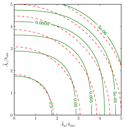
Figure 3: Comparison of the $\mathcal{B}$ (solid) and $\mathcal{F}$ (dashed) statistics at equal false-alarm probabilities. In the simple case of a diagonal amplitude parameter metric (104), we can explicitly evaluate the $\mathcal{B}$-statistic via (113) and the $\mathcal{F}$-statistic via (107). Because a prior distribution constant in the physical coordinates $\{h_{0},\chi,\psi,\phi_{0}\}$ weights circular polarization ($A_{\textsc{r}}$ or $A_{\textsc{l}}$ small) more heavily does than a prior uniform in the signal amplitudes $\{\mathcal{A}^{\breve{\mu}}\}$, we find that nearly circularly-polarized signals produce a $\mathcal{B}$ statistic value more significant than their $\mathcal{F}$-statistic value, compared to nearly linearly-polarized signals (for which $A_{\textsc{r}}$ and $A_{\textsc{l}}$ are comparable).

VI.2 Comparison to Root-Radius Gaussian Approximation

We can compare the explicit result (113) to the approximate result (96) obtained in section V.3 by Gaussian integration in root-radius coordinates. Applying the explicit form (109) the Gaussian approximation becomes

$$\frac{\mathcal{B}_{\textsc{r}}(\widehat{A}_{\textsc{r}})}{\mathcal{B}_{\textsc{r}}(0)}\approx\frac{2\pi Ah_{\text{det}}^{2}}{\widehat{A}_{\textsc{r}}^{3/2}}\,e^{\mathcal{F}_{\textsc{r}}(\widehat{A}_{\textsc{r}})}=\frac{2^{3/4}}{\Gamma(\frac{1}{4})}\left(\frac{\widehat{A}_{\textsc{r}}}{h_{\text{det}}}\right)^{\!-3/2}\!e^{\widehat{A}_{\textsc{r}}^{2}/2h_{\text{det}}^{2}}\ .$$ (114)

We see that this agrees with the general result at large $\widehat{A}_{\textsc{r}}$, since

$${}_{1}F_{1}\left(\frac{1}{4},1,\frac{\widehat{A}_{\textsc{r}}^{2}}{2h_{\text{det}}^{2}}\right)\stackrel{{\scriptstyle\widehat{A}_{\textsc{r}}\rightarrow\infty}}{{\longrightarrow}}\frac{2^{3/4}}{\Gamma(\frac{1}{4})}\left(\frac{\widehat{A}_{\textsc{r}}}{h_{\text{det}}}\right)^{\!-3/2}\!e^{\widehat{A}_{\textsc{r}}^{2}/2h_{\text{det}}^{2}}$$ (115)

by identity (13.5.1) of abramowitz64:_handb_mathem_funct . In figure 4 we plot the exact form (112) of $\frac{\mathcal{B}_{\textsc{r}}(\widehat{A}_{\textsc{r}})}{\mathcal{B}_{\textsc{r}}(0)}e^{-\mathcal{F}(\widehat{A}_{\textsc{r}})}$ as well as the limiting form (114).

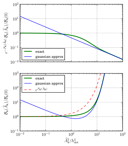
Figure 4: Comparison of the exact form of $\frac{\mathcal{B}_{\textsc{r}}(\widehat{A}_{\textsc{r}})}{\mathcal{B}_{\textsc{r}}(0)}$ to the result of the approximate Gaussian integral, both with the factor of $e^{\mathcal{F}(\widehat{A}_{\textsc{r}})}=e^{\widehat{A}_{\textsc{r}}/2h_{\text{det}}^{2}}$ factored out and without. Note that the value of the detection statistic matters, because the overall statistic is $\mathcal{B}({x})=\mathcal{B}_{\textsc{r}}(\widehat{A}_{\textsc{r}})\mathcal{B}_{\textsc{l}}(\widehat{A}_{\textsc{l}})$.

VI.3 Range of Validity of CPF Coordinate Gaussian Approximation

Recall that in section V.2 we expand the combination $\Lambda(\mathcal{A};{x})+\alpha(\mathcal{A})$ about the maximum-likelihood point $\mathcal{A}=\widehat{\mathcal{A}}$, where $\alpha(\mathcal{A})$ is the logarithm of the measure of the $\mathcal{B}$-statistic integral, given by (81). Subject to the simplifying assumptions of this section, the log-likelihood ratio becomes

$$\begin{split}\Lambda(\mathcal{A};{x})&=\mathcal{F}({x})-\frac{1}{2h_{\text{det}}^{2}}\bigl{(}[\mathcal{A}^{\breve{1}}-\widehat{\mathcal{A}}^{\breve{1}}({x})]^{2}+[\mathcal{A}^{\breve{2}}-\widehat{\mathcal{A}}^{\breve{2}}({x})]^{2}\\ &\phantom{=\mathcal{F}({x})-\frac{1}{2h_{\text{det}}^{2}}\bigl{(}}+[\mathcal{A}^{\breve{3}}-\widehat{\mathcal{A}}^{\breve{3}}({x})]^{2}+[\mathcal{A}^{\breve{4}}-\widehat{\mathcal{A}}^{\breve{4}}({x})]^{2}\bigr{)}\\ &=\mathcal{F}({x})+\Lambda_{\textsc{r}}(\mathcal{A}^{\breve{1}},\mathcal{A}^{\breve{2}};{x})+\Lambda_{\textsc{l}}(\mathcal{A}^{\breve{3}},\mathcal{A}^{\breve{4}};{x})\end{split}$$ (116)

and we can examine the behavior of $\Lambda_{\textsc{r}}(\mathcal{A}^{\breve{1}},\mathcal{A}^{\breve{2}};{x})+\alpha_{\textsc{r}}(\mathcal{A}^{\breve{1}},\mathcal{A}^{\breve{2}})$ and $\Lambda_{\textsc{l}}(\mathcal{A}^{\breve{3}},\mathcal{A}^{\breve{4}};{x})+\alpha_{\textsc{l}}(\mathcal{A}^{\breve{3}},\mathcal{A}^{\breve{4}})$ separately. To examine the integral for a particular data realization ${x}$, we can define rotated CPF coordinates

$$\mathcal{A}^{\widehat{1}}=A_{\textsc{r}}\cos(\phi_{\textsc{r}}-\widehat{\phi}_{\textsc{r}}) =\mathcal{A}^{\breve{1}}\cos\widehat{\phi}_{\textsc{r}}+\mathcal{A}^{\breve{2}}\sin\widehat{\phi}_{\textsc{r}}$$ (117a)

$$\mathcal{A}^{\widehat{2}}=A_{\textsc{r}}\sin(\phi_{\textsc{r}}-\widehat{\phi}_{\textsc{r}}) =-\mathcal{A}^{\breve{1}}\sin\widehat{\phi}_{\textsc{r}}+\mathcal{A}^{\breve{2}}\cos\widehat{\phi}_{\textsc{r}}$$ (117b)

so that

$$\Lambda_{\textsc{r}}(\mathcal{A}^{\widehat{1}},\mathcal{A}^{\widehat{2}};\widehat{A}_{\textsc{r}})+\alpha_{\textsc{r}}(\mathcal{A}^{\widehat{1}},\mathcal{A}^{\widehat{2}})\\ =-\frac{1}{2h_{\text{det}}^{2}}\left([\mathcal{A}^{\widehat{1}}-\widehat{A}_{\textsc{r}}]^{2}+[\mathcal{A}^{\widehat{2}}]^{2}\right)-\frac{3}{4}\ln\left([\mathcal{A}^{\widehat{1}}]^{2}+[\mathcal{A}^{\widehat{2}}]^{2}\right)\ .$$ (118)

We can find the stationary points explicitly, since

$$\frac{\partial(\Lambda_{\textsc{r}}+\alpha_{\textsc{r}})}{\partial\mathcal{A}^{\widehat{1}}} =-\frac{\mathcal{A}^{\widehat{1}}-\widehat{A}_{\textsc{r}}}{h_{\text{det}}^{2}}-\frac{3}{2}\frac{\mathcal{A}^{\widehat{1}}}{(\mathcal{A}^{\widehat{1}})^{2}+(\mathcal{A}^{\widehat{2}})^{2}}$$ (119a)

$$\frac{\partial(\Lambda_{\textsc{r}}+\alpha_{\textsc{r}})}{\partial\mathcal{A}^{\widehat{2}}} =-\frac{\mathcal{A}^{\widehat{2}}}{h_{\text{det}}^{2}}-\frac{3}{2}\frac{\mathcal{A}^{\widehat{2}}}{(\mathcal{A}^{\widehat{1}})^{2}+(\mathcal{A}^{\widehat{2}})^{2}}$$ (119b)

we see that $\frac{\partial(\Lambda_{\textsc{r}}+\alpha_{\textsc{r}})}{\partial\mathcal{A}^{\widehat{2}}}=0$ when $\mathcal{A}^{\widehat{2}}=0$, which means that the stationary points occur when

$$-\frac{\mathcal{A}^{\widehat{1}}-\widehat{A}_{\textsc{r}}}{h_{\text{det}}^{2}}-\frac{3}{2\mathcal{A}^{\widehat{1}}}=0$$ (120)

i.e., at the solutions of the quadratic equation

$$2(\mathcal{A}^{\widehat{1}})^{2}-2\widehat{A}_{\textsc{r}}(\mathcal{A}^{\widehat{1}})+3h_{\text{det}}^{2}=0$$ (121)

which are

$$\mathcal{A}^{\widehat{1}}=\frac{\widehat{A}_{\textsc{r}}\pm\sqrt{\widehat{A}_{\textsc{r}}^{2}-6h_{\text{det}}^{2}}}{2}$$ (122)

Since $\Lambda_{\textsc{r}}(\mathcal{A}^{\widehat{1}},0;\widehat{A}_{\textsc{r}})+\alpha_{\textsc{r}}(\mathcal{A}^{\widehat{1}},0)$ goes to $+\infty$ as $\mathcal{A}^{\widehat{1}}\rightarrow 0$ and $-\infty$ as $\mathcal{A}^{\widehat{1}}\rightarrow+\infty$, it is apparent that $\mathcal{A}^{\widehat{1}}=\frac{\widehat{A}_{\textsc{r}}-\sqrt{\widehat{A}_{\textsc{r}}^{2}-6h_{\text{det}}^{2}}}{2}$ is a local minimum and $\mathcal{A}^{\widehat{1}}=\mathcal{A}^{\widehat{1}}_{\text{max}}=\frac{\widehat{A}_{\textsc{r}}+\sqrt{\widehat{A}_{\textsc{r}}^{2}-6h_{\text{det}}^{2}}}{2}$ is a local maximum.

We also see that if $\widehat{A}_{\textsc{r}}/h_{\text{det}}<\sqrt{6}\approx 2.450$, there is no local maximum, only the singularity at the origin of the $\{\mathcal{A}^{\widehat{1}},\mathcal{A}^{\widehat{2}}\}$ plane. Note that this condition is actually more restrictive than the one corresponding to a saddle point in the quadratic expansion at the maximum likelihood point. That is determined by the sign of

$$\mathcal{N}_{\breve{1}\breve{1}}=-\frac{1}{h_{\text{det}}^{2}}+\frac{3}{2\widehat{A}_{\textsc{r}}^{2}}$$ (123)

To follow the calculation of section V.2, we define the quadratic expansion of $\alpha_{\textsc{r}}(\mathcal{A}^{\widehat{1}},\mathcal{A}^{\widehat{2}})$ about a point $(\mathcal{A}^{\widehat{1}}_{0},\mathcal{A}^{\widehat{2}}_{0})$ as

$$\alpha_{\textsc{r}}^{\text{quad}}(\mathcal{A}^{\widehat{1}},\mathcal{A}^{\widehat{2}};\mathcal{A}^{\widehat{1}}_{0},\mathcal{A}^{\widehat{2}}_{0})\\ =\alpha_{\textsc{r}}(\mathcal{A}^{\widehat{1}}_{0},\mathcal{A}^{\widehat{2}}_{0})+\alpha_{\textsc{r}}{}_{,\widehat{\mu}}(\mathcal{A}^{\widehat{1}}_{0},\mathcal{A}^{\widehat{2}}_{0})[\mathcal{A}^{\widehat{\mu}}-\mathcal{A}^{\widehat{\mu}}_{0}]\\ +\frac{1}{2}\alpha_{\textsc{r}}{}_{,\widehat{\mu}\widehat{\nu}}(\mathcal{A}^{\widehat{1}}_{0},\mathcal{A}^{\widehat{2}}_{0})[\mathcal{A}^{\widehat{\mu}}-\mathcal{A}^{\widehat{\mu}}_{0}][\mathcal{A}^{\widehat{\nu}}-\mathcal{A}^{\widehat{\nu}}_{0}]$$ (124)

In particular

$$\alpha_{\textsc{r}}^{\text{quad}}(\mathcal{A}^{\widehat{1}},\mathcal{A}^{\widehat{2}};\mathcal{A}^{\widehat{1}}_{0},0)=-\frac{3}{2}\ln\mathcal{A}^{\widehat{1}}_{0}\\ -\frac{3}{2\mathcal{A}^{\widehat{1}}_{0}}(\mathcal{A}^{\widehat{1}}-\mathcal{A}^{\widehat{1}}_{0})+\frac{3}{4[\mathcal{A}^{\widehat{1}}_{0}]^{2}}(\mathcal{A}^{\widehat{1}}-\mathcal{A}^{\widehat{1}}_{0})^{2}$$ (125)

If $\widehat{A}_{\textsc{r}}/h_{\text{det}}>\sqrt{6}\approx 2.450$, so that $\mathcal{A}^{\widehat{1}}_{\text{max}}=\frac{\widehat{A}_{\textsc{r}}+\sqrt{\widehat{A}_{\textsc{r}}^{2}-6h_{\text{det}}^{2}}}{2}$ is a real number, the point $(\mathcal{A}^{\widehat{1}},\mathcal{A}^{\widehat{2}})=(\mathcal{A}^{\widehat{1}}_{\text{max}},0)$ is a local maximum of $\Lambda(\mathcal{A}^{\widehat{1}},\mathcal{A}^{\widehat{2}})+\alpha(\mathcal{A}^{\widehat{1}},\mathcal{A}^{\widehat{2}})$, and the quadratic expression

$$\Lambda(\mathcal{A}^{\widehat{1}},\mathcal{A}^{\widehat{2}})+\alpha^{\text{quad}}(\mathcal{A}^{\widehat{1}},\mathcal{A}^{\widehat{2}};\mathcal{A}^{\widehat{1}}_{\text{max}},0)$$ (126)

is an approximation to $\Lambda(\mathcal{A}^{\widehat{1}},\mathcal{A}^{\widehat{2}})+\alpha(\mathcal{A}^{\widehat{1}},\mathcal{A}^{\widehat{2}})$ near its local maximum at $(\mathcal{A}^{\widehat{1}},\mathcal{A}^{\widehat{2}})=(\mathcal{A}^{\widehat{1}}_{\text{max}},0)$. This is the situation illustrated in figure 5, which plots $\Lambda(\mathcal{A}^{\widehat{1}},0;\widehat{A}_{\textsc{r}})+\alpha(\mathcal{A}^{\widehat{1}},0)$ and its various quadratic approximations when $\widehat{A}_{\textsc{r}}=3h_{\text{det}}$.

We can always define a quadratic expansion about the maximum likelihood point $(\mathcal{A}^{\widehat{1}},\mathcal{A}^{\widehat{2}})=(\widehat{A}_{\textsc{r}},0)$, namely,

$$\Lambda(\mathcal{A}^{\widehat{1}},\mathcal{A}^{\widehat{2}})+\alpha^{\text{quad}}(\mathcal{A}^{\widehat{1}},\mathcal{A}^{\widehat{2}};\widehat{A}_{\textsc{r}},0)=\frac{\widehat{A}_{\textsc{r}}^{2}}{2h_{\text{det}}^{2}}-\frac{3}{2}\ln\widehat{A}_{\textsc{r}}\\ -\frac{3}{2\widehat{A}_{\textsc{r}}}(\mathcal{A}^{\widehat{1}}-\widehat{A}_{\textsc{r}})+\frac{1}{2}\left(\frac{3}{2[\widehat{A}_{\textsc{r}}]^{2}}-\frac{1}{h_{\text{det}}^{2}}\right)(\mathcal{A}^{\widehat{1}}-\widehat{A}_{\textsc{r}})^{2}\\$$ (127)

which will have a stationary point at $(\mathcal{A}^{\widehat{1}},\mathcal{A}^{\widehat{2}})=\left(\widehat{A}_{\textsc{r}}\left[\frac{6h_{\text{det}}^{2}-2\widehat{A}_{\textsc{r}}^{2}}{3h_{\text{det}}^{2}-2\widehat{A}_{\textsc{r}}^{2}}\right],0\right)$. If $\widehat{A}_{\textsc{r}}/h_{\text{det}}<\sqrt{3/2}\approx 1.225$, this is a saddle point, as illustrated in figure 6, which plots $\Lambda(\mathcal{A}^{\widehat{1}},0;\widehat{A}_{\textsc{r}})+\alpha^{\text{quad}}(\mathcal{A}^{\widehat{1}},0)$ and the quadratic approximation $\Lambda(\mathcal{A}^{\widehat{1}},0;\widehat{A}_{\textsc{r}})+\alpha^{\text{quad}}(\mathcal{A}^{\widehat{1}},0;\widehat{A}_{\textsc{r}},0)$ when $\widehat{A}_{\textsc{r}}=h_{\text{det}}$. Because the quadratic approximation curves upwards in the $\mathcal{A}^{\widehat{1}}$ direction, it cannot be used to calculate a Gaussian integral.

Figure 7 shows an intermediate value $\widehat{A}_{\textsc{r}}=2h_{\text{det}}$, where the quadratic approximation $\Lambda_{\textsc{r}}(\mathcal{A}^{\widehat{1}},\mathcal{A}^{\widehat{2}};\widehat{A}_{\textsc{r}})+\alpha_{\textsc{r}}^{\text{quad}}(\mathcal{A}^{\widehat{1}},\mathcal{A}^{\widehat{2}};\widehat{A}_{\textsc{r}},0)$ has a local maximum, but $\Lambda_{\textsc{r}}(\mathcal{A}^{\widehat{1}},\mathcal{A}^{\widehat{2}};\widehat{A}_{\textsc{r}})+\alpha_{\textsc{r}}(\mathcal{A})$ does not.

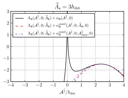
Figure 5: Quadratic approximations to $\Lambda_{\textsc{r}}(\mathcal{A}^{\widehat{1}},0;\widehat{A}_{\textsc{r}})+\alpha_{\textsc{r}}(\mathcal{A}^{\widehat{1}},0)$ when $\widehat{A}_{\textsc{r}}=3h_{\text{det}}$, as a function of the rotated CPF coordinate $\mathcal{A}^{\widehat{1}}=A_{\textsc{r}}\cos(\phi_{\textsc{r}}-\widehat{\phi}_{\textsc{r}})$ defined in (117), along the line $\mathcal{A}^{\widehat{2}}=A_{\textsc{r}}\sin(\phi_{\textsc{r}}-\widehat{\phi}_{\textsc{r}})=0$. We show two different quadratic approximations: one based on expanding $\alpha_{\textsc{r}}(\mathcal{A}^{\widehat{1}},0)$ about the maximum likelihood point $\mathcal{A}^{\widehat{1}}=\widehat{A}_{\textsc{r}}=3h_{\text{det}}$ and the other about $\mathcal{A}^{\widehat{1}}_{\text{max}}=\frac{3+\sqrt{3}}{2}\approx 2.366h_{\text{det}}$, at which $\Lambda_{\textsc{r}}(\mathcal{A}^{\widehat{1}},0;\widehat{A}_{\textsc{r}})+\alpha_{\textsc{r}}(\mathcal{A}^{\widehat{1}},0)$ has a local maximum. [Note that $\Lambda_{\textsc{r}}(\mathcal{A}^{\widehat{1}},\mathcal{A}^{\widehat{2}};\widehat{A}_{\textsc{r}})+\alpha_{\textsc{r}}^{\text{quad}}(\mathcal{A}^{\widehat{1}},\mathcal{A}^{\widehat{2}};\widehat{A}_{\textsc{r}},0)$ has a local maximum at $(\mathcal{A}^{\widehat{1}},\mathcal{A}^{\widehat{2}})=(2.4h_{\text{det}},0)$.]

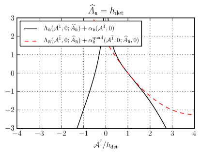
Figure 6: Quadratic approximation to $\Lambda_{\textsc{r}}(\mathcal{A}^{\widehat{1}},0;\widehat{A}_{\textsc{r}})+\alpha_{\textsc{r}}(\mathcal{A}^{\widehat{1}},0)$ when $\widehat{A}_{\textsc{r}}=h_{\text{det}}$. Here $\Lambda_{\textsc{r}}(\mathcal{A}^{\widehat{1}},0;\widehat{A}_{\textsc{r}})+\alpha_{\textsc{r}}(\mathcal{A}^{\widehat{1}},0)$ has no local maximum, only the singularity at $\mathcal{A}^{\widehat{1}}=0$, and the stationary point of $\Lambda_{\textsc{r}}(\mathcal{A}^{\widehat{1}},\mathcal{A}^{\widehat{2}};\widehat{A}_{\textsc{r}})+\alpha_{\textsc{r}}^{\text{quad}}(\mathcal{A}^{\widehat{1}},\mathcal{A}^{\widehat{2}};\widehat{A}_{\textsc{r}},0)$, located at $(\mathcal{A}^{\widehat{1}},\mathcal{A}^{\widehat{2}})=(4h_{\text{det}},0)$, is a saddle point, since it curves upwards in the $\mathcal{A}^{\widehat{1}}$ direction and downward in the $\mathcal{A}^{\widehat{2}}$ direction.

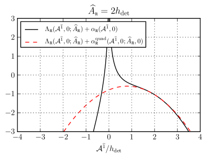
Figure 7: Quadratic approximation to $\Lambda_{\textsc{r}}(\mathcal{A}^{\widehat{1}},0;\widehat{A}_{\textsc{r}})+\alpha_{\textsc{r}}(\mathcal{A}^{\widehat{1}},0)$ when $\widehat{A}_{\textsc{r}}=2h_{\text{det}}$. Even though $\Lambda_{\textsc{r}}(\mathcal{A}^{\widehat{1}},0;\widehat{A}_{\textsc{r}})+\alpha_{\textsc{r}}(\mathcal{A}^{\widehat{1}},0)$ has no local maximum, the quadratic approximation $\Lambda_{\textsc{r}}(\mathcal{A}^{\widehat{1}},\mathcal{A}^{\widehat{2}};\widehat{A}_{\textsc{r}})+\alpha_{\textsc{r}}^{\text{quad}}(\mathcal{A}^{\widehat{1}};\widehat{A}_{\textsc{r}},0)$ has a local maximum at $(\mathcal{A}^{\widehat{1}},\mathcal{A}^{\widehat{2}})=(0.8h_{\text{det}},0)$. However, it is not a useful approximation to the original function for evaluating the integral, even though it is accurate close to the maximum likelihood point $\mathcal{A}^{\widehat{1}}=2h_{\text{det}}$.

VII Conclusions

We have demonstrated several new sets of coordinates on the amplitude parameter space of continuous gravitational waves. By taking linear combinations (29) of the usual Jaranowski-Królak-Schutz (JKS) coordinates, we obtain a set of variables, called CPF (circular polarization factored) coordinates which are still coefficients in a linear representation (30) of the signal waveform, but which are more closely connected to the physical amplitude parameters of signal amplitude $h_{0}$, inclination and polarization angles $\iota$ and $\psi$, and initial phase $\phi_{0}$. In particular, these new coordinates divide naturally into two pairs of Cartesian-like coordinates (one corresponding to right- and one to left-circular polarization), and the polar coordinates (36) on these two subspaces, which we call CPF-polar coordinates, are closely connected to the physical amplitude parameters: the radial coordinates $A_{\textsc{r}}$ and $A_{\textsc{l}}$ are functions of $h_{0}$ and $\chi=\cos\iota$, while the angular coordinates $\phi_{\textsc{r}}$ and $\phi_{\textsc{l}}$ are functions of $\psi$ and $\phi_{0}$, as shown in (37). We also introduce so-called root-radius coordinates $\{x_{\textsc{r}},y_{\textsc{r}},x_{\textsc{l}},y_{\textsc{l}}\}$, derived from polar coordinates $\{r_{\textsc{r}}=A_{\textsc{r}}^{1/4},\phi_{\textsc{r}},r_{\textsc{l}}=A_{\textsc{l}}^{1/4},\phi_{\textsc{l}}\}$, which have the simplifying feature that the Jacobian of the transformation between root-radius coordinates and the physical coordinates $\{h_{0},\chi=\cos\iota,\psi,\phi_{0}\}$ is a constant.

We have presented several demonstrations of the utility of these new coordinates. They can be used in a simple derivation of the Jacobian determinant (53) for the transformation between JKS and physical coordinates (previously computed using computer algebra). The coordinate singularities and ambiguities in physical parameters associated with right or left circular polarization can be understood as the origins of the two polar coordinate systems, (58) and (59), respectively. Finally, if we express in these coordinates the log-likelihood ratio between models of Gaussian noise with and without a continuous gravitational-wave signal, we can obtain results useful for the calculation of the $\mathcal{B}$-statistic, which is the Bayes factor for a comparison between the models.

Past workPrix09:_Bstat has shown that if an unphysical prior is used for the $\mathcal{B}$-statistic integral, an explicit Gaussian integration in JKS coordinates (for which there is a straightforward equivalent in CPF coordinates) shows that the $\mathcal{B}$ statistic is equivalent to the $\mathcal{F}$ statistic. If a more physically reasonable prior is used, in particular one isotropic in the orientation angles $\iota$ and $\psi$, the resulting Jacobian factor complicates the evaluation of the integral. We limited attention to the case where the prior is uniform in the physical coordinates $\{h_{0},\chi=\cos\iota,\psi,\phi_{0}\}$, and showed that the coordinate singularities in the resulting measure make even an approximate Gaussian integration in CPF (or JKS) coordinates problematic. We have showed that an approximate Gaussian integration can be performed in root-radius coordinates, with the result that, up to an irrelevant constant, $\ln\mathcal{B}\approx\mathcal{F}-\frac{3}{2}\ln(\widehat{A}_{\textsc{r}}\widehat{A}_{\textsc{l}})$, where $\widehat{A}_{\textsc{r}}$ and $\widehat{A}_{\textsc{l}}$ are the maximum-likelihood estimates of the CPF-polar radial coordinates $A_{\textsc{r}}=h_{0}\left(\frac{1+\chi}{2}\right)^{2}$ and $A_{\textsc{l}}=h_{0}\left(\frac{1-\chi}{2}\right)^{2}$. This provides insights into the $\mathcal{B}$ statistic in the regime where the signal is strong and not too close to circular polarization. Finally, we considered the $\mathcal{B}$-statistic in the physical coordinates themselves and showed that two of the four integrals could be performed exactly.

To gain more explicit insight into the behavior of the various $\mathcal{B}$-statistic integrals, we considered a special case where the amplitude parameter metric is diagonal, and showed that the simple form of the log-likelihood ratio in this case allowed the integrals to be performed analytically in CPF-polar coordinates, leading to an explicit exact result (113) in terms of the confluent hypergeometric function. This could then be compared to the approximate result from the Gaussian expansion in root-radius coordinates to show the breakdown of the approximation for weak or nearly-circularly-polarized signals.

Appendix A Explicit form of Amplitude Parameter Metric

The explicit forms of the matrix elements (64) can be obtained explicitly by dividing the data from each detector $X$ into short stretches of data $[t_{l},\,t_{l}+T_{\text{sft}})$ of length $T_{\text{sft}}$ and Fourier transformed (hence usually referred to as “Short Fourier Transforms”, or SFTs). For a nearly monochromatic signal around frequency $f_{0}$, we can define the usual (multi-detector) scalar product as

$$\left(x|y\right)\equiv\sum_{Xl}\frac{4}{S^{X}_{l}(f_{0})}\operatorname{Re}\int_{0}^{\infty}\widetilde{x}^{X*}_{l}(f)\,\widetilde{y}^{X}_{l}(f)\,df\ ,$$ (128)

where $S^{X}_{l}(f_{0})$ is the one-sided noise power spectral density around the frequency $f_{0}$ in detector $X$ during time stretch $l$, and $\widetilde{x}_{l}^{X},\widetilde{y}_{l}^{X}$ are the corresponding Fourier-transforms of $x^{X}(t),y^{X}(t)$ restricted to the SFT time-stretch $l$.

The explicit form of the scalar basis functions over each SFT time stretch $t\in[t_{l},\,t_{l}+T_{\text{sft}})$, defined according to (9) as $\widetilde{h}^{X}_{\mu,l}(f)\equiv\widetilde{{\mathchoice{\mathord{\hbox to0.0pt{\hbox to8.79988pt{\hss$\displaystyle h$\hss}\hss}\raise 7.98605pt\hbox to8.79988pt{\hss\hbox{$\scriptstyle\leftrightarrow$}\hss}}}{\mathord{\hbox to0.0pt{\hbox to8.79988pt{\hss$\textstyle h$\hss}\hss}\raise 7.98605pt\hbox to8.79988pt{\hss\hbox{$\scriptstyle\leftrightarrow$}\hss}}}{\mathord{\hbox to0.0pt{\hbox to6.99988pt{\hss$\scriptstyle h$\hss}\hss}\raise 5.59023pt\hbox to6.99988pt{\hss\hbox{$\scriptscriptstyle\leftrightarrow$}\hss}}}{\mathord{\hbox to0.0pt{\hbox to6.99988pt{\hss$\scriptscriptstyle h$\hss}\hss}\raise 3.99301pt\hbox to6.99988pt{\hss\hbox{$\scriptscriptstyle\leftrightarrow$}\hss}}}}\mathord{\hbox{}}}{}^{X}_{\mu,l}(f):{\mathchoice{\mathord{\hbox to0.0pt{\hbox to8.79988pt{\hss$\displaystyle d$\hss}\hss}\raise 7.98605pt\hbox to8.79988pt{\hss\hbox{$\scriptstyle\leftrightarrow$}\hss}}}{\mathord{\hbox to0.0pt{\hbox to8.79988pt{\hss$\textstyle d$\hss}\hss}\raise 7.98605pt\hbox to8.79988pt{\hss\hbox{$\scriptstyle\leftrightarrow$}\hss}}}{\mathord{\hbox to0.0pt{\hbox to6.99988pt{\hss$\scriptstyle d$\hss}\hss}\raise 5.59023pt\hbox to6.99988pt{\hss\hbox{$\scriptscriptstyle\leftrightarrow$}\hss}}}{\mathord{\hbox to0.0pt{\hbox to6.99988pt{\hss$\scriptscriptstyle d$\hss}\hss}\raise 3.99301pt\hbox to6.99988pt{\hss\hbox{$\scriptscriptstyle\leftrightarrow$}\hss}}}}\mathord{\hbox{}}_{l}^{X}(f)$, can be given in the time-domain as

$$h^{X}_{1,l}(t) =a^{X}_{l}(f_{0})\,\cos\phi^{X}(t)\ ,$$ (129a)

$$h^{X}_{2,l}(t) =b^{X}_{l}(f_{0})\,\cos\phi^{X}(t)\ ,$$ (129b)

$$h^{X}_{3,l}(t) =a^{X}_{l}(f_{0})\,\sin\phi^{X}(t)\ ,$$ (129c)

$$h^{X}_{4,l}(t) =b^{X}_{l}(f_{0})\,\sin\phi^{X}(t)\ ,$$ (129d)

where we defined the shorthand $\phi^{X}(t)\equiv\phi(\tau^{X}(t))$, and where the frequency-dependent complex AM coefficients for time stretch $l$ are (see (12)) $a^{X}_{l}(f)={\mathchoice{\mathord{\hbox to0.0pt{\hbox to8.79988pt{\hss$\displaystyle\varepsilon$\hss}\hss}\raise 4.95134pt\hbox to8.79988pt{\hss\hbox{$\scriptstyle\leftrightarrow$}\hss}}}{\mathord{\hbox to0.0pt{\hbox to8.79988pt{\hss$\textstyle\varepsilon$\hss}\hss}\raise 4.95134pt\hbox to8.79988pt{\hss\hbox{$\scriptstyle\leftrightarrow$}\hss}}}{\mathord{\hbox to0.0pt{\hbox to6.99988pt{\hss$\scriptstyle\varepsilon$\hss}\hss}\raise 3.46594pt\hbox to6.99988pt{\hss\hbox{$\scriptscriptstyle\leftrightarrow$}\hss}}}{\mathord{\hbox to0.0pt{\hbox to6.99988pt{\hss$\scriptscriptstyle\varepsilon$\hss}\hss}\raise 2.47566pt\hbox to6.99988pt{\hss\hbox{$\scriptscriptstyle\leftrightarrow$}\hss}}}}\mathord{\hbox{}}_{\!+}:{\mathchoice{\mathord{\hbox to0.0pt{\hbox to8.79988pt{\hss$\displaystyle d$\hss}\hss}\raise 7.98605pt\hbox to8.79988pt{\hss\hbox{$\scriptstyle\leftrightarrow$}\hss}}}{\mathord{\hbox to0.0pt{\hbox to8.79988pt{\hss$\textstyle d$\hss}\hss}\raise 7.98605pt\hbox to8.79988pt{\hss\hbox{$\scriptstyle\leftrightarrow$}\hss}}}{\mathord{\hbox to0.0pt{\hbox to6.99988pt{\hss$\scriptstyle d$\hss}\hss}\raise 5.59023pt\hbox to6.99988pt{\hss\hbox{$\scriptscriptstyle\leftrightarrow$}\hss}}}{\mathord{\hbox to0.0pt{\hbox to6.99988pt{\hss$\scriptscriptstyle d$\hss}\hss}\raise 3.99301pt\hbox to6.99988pt{\hss\hbox{$\scriptscriptstyle\leftrightarrow$}\hss}}}}\mathord{\hbox{}}_{l}(f)$ and $b^{X}_{l}(f)={\mathchoice{\mathord{\hbox to0.0pt{\hbox to8.79988pt{\hss$\displaystyle\varepsilon$\hss}\hss}\raise 4.95134pt\hbox to8.79988pt{\hss\hbox{$\scriptstyle\leftrightarrow$}\hss}}}{\mathord{\hbox to0.0pt{\hbox to8.79988pt{\hss$\textstyle\varepsilon$\hss}\hss}\raise 4.95134pt\hbox to8.79988pt{\hss\hbox{$\scriptstyle\leftrightarrow$}\hss}}}{\mathord{\hbox to0.0pt{\hbox to6.99988pt{\hss$\scriptstyle\varepsilon$\hss}\hss}\raise 3.46594pt\hbox to6.99988pt{\hss\hbox{$\scriptscriptstyle\leftrightarrow$}\hss}}}{\mathord{\hbox to0.0pt{\hbox to6.99988pt{\hss$\scriptscriptstyle\varepsilon$\hss}\hss}\raise 2.47566pt\hbox to6.99988pt{\hss\hbox{$\scriptscriptstyle\leftrightarrow$}\hss}}}}\mathord{\hbox{}}_{\!\times}:{\mathchoice{\mathord{\hbox to0.0pt{\hbox to8.79988pt{\hss$\displaystyle d$\hss}\hss}\raise 7.98605pt\hbox to8.79988pt{\hss\hbox{$\scriptstyle\leftrightarrow$}\hss}}}{\mathord{\hbox to0.0pt{\hbox to8.79988pt{\hss$\textstyle d$\hss}\hss}\raise 7.98605pt\hbox to8.79988pt{\hss\hbox{$\scriptstyle\leftrightarrow$}\hss}}}{\mathord{\hbox to0.0pt{\hbox to6.99988pt{\hss$\scriptstyle d$\hss}\hss}\raise 5.59023pt\hbox to6.99988pt{\hss\hbox{$\scriptscriptstyle\leftrightarrow$}\hss}}}{\mathord{\hbox to0.0pt{\hbox to6.99988pt{\hss$\scriptscriptstyle d$\hss}\hss}\raise 3.99301pt\hbox to6.99988pt{\hss\hbox{$\scriptscriptstyle\leftrightarrow$}\hss}}}}\mathord{\hbox{}}_{l}(f)$, respectively. These reduce to the real-valued constants $a^{X}_{l}$ and $b^{X}_{l}$ in the long-wavelength limit. Using this together with the definition of the amplitude-parameter metric (63) and (64) we find

$$A =\sum_{Xl}\frac{T_{\text{sft}}}{S^{X}_{l}(f_{0})}\left\lvert a^{X}_{l}(f_{0})\right\rvert^{2}\ ,$$ (130a)

$$B =\sum_{Xl}\frac{T_{\text{sft}}}{S^{X}_{l}(f_{0})}\left\lvert b^{X}_{l}(f_{0})\right\rvert^{2}\ ,$$ (130b)

$$C =\sum_{Xl}\frac{T_{\text{sft}}}{S^{X}_{l}(f_{0})}\operatorname{Re}\left[a^{X*}_{l}(f_{0})\,b^{X}_{l}(f_{0})\right]\ ,$$ (130c)

$$E =\sum_{Xl}\frac{T_{\text{sft}}}{S^{X}_{l}(f_{0})}\operatorname{Im}\left[a^{X*}_{l}(f_{0})\,b^{X}_{l}(f_{0})\right]\ ,$$ (130d)

The explicit forms of the matrix elements $\mathcal{M}_{\breve{\mu}\breve{\nu}}=\left(h_{\breve{\mu}}|h_{\breve{\nu}}\right)$ can be obtained by using either (31) or (33), namely

$$\begin{split}I&=A+B+2E=\sum_{Xl}\frac{T_{\text{sft}}}{S^{X}_{l}(f_{0})}\left\lvert a^{X}_{{\textsc{l}},l}(f_{0})\right\rvert^{2}\ ,\end{split}$$ (131a)

$$\begin{split}J&=A+B-2E=\sum_{Xl}\frac{T_{\text{sft}}}{S^{X}_{l}(f_{0})}\left\lvert a^{X}_{{\textsc{r}},l}(f_{0})\right\rvert^{2}\ ,\end{split}$$ (131b)

$$\begin{split}K&=2C=\sum_{Xl}\frac{T_{\text{sft}}}{S^{X}_{l}(f_{0})}\operatorname{Re}\left[a^{X*}_{{\textsc{l}},l}(f_{0})\,a^{X}_{{\textsc{r}},l}(f_{0})\right]\ ,\end{split}$$ (131c)

$$\begin{split}L&=A-B=\sum_{Xl}\frac{T_{\text{sft}}}{S^{X}_{l}(f_{0})}\operatorname{Im}\left[a^{X*}_{{\textsc{l}},l}(f_{0})a^{X}_{{\textsc{r}},l}(f_{0})\right],\end{split}$$ (131d)

where

$$a^{X}_{{\textsc{r}},l}(f_{0})={\mathchoice{\mathord{\hbox to0.0pt{\hbox to8.79988pt{\hss$\displaystyle\varepsilon$\hss}\hss}\raise 4.95134pt\hbox to8.79988pt{\hss\hbox{$\scriptstyle\leftrightarrow$}\hss}}}{\mathord{\hbox to0.0pt{\hbox to8.79988pt{\hss$\textstyle\varepsilon$\hss}\hss}\raise 4.95134pt\hbox to8.79988pt{\hss\hbox{$\scriptstyle\leftrightarrow$}\hss}}}{\mathord{\hbox to0.0pt{\hbox to6.99988pt{\hss$\scriptstyle\varepsilon$\hss}\hss}\raise 3.46594pt\hbox to6.99988pt{\hss\hbox{$\scriptscriptstyle\leftrightarrow$}\hss}}}{\mathord{\hbox to0.0pt{\hbox to6.99988pt{\hss$\scriptscriptstyle\varepsilon$\hss}\hss}\raise 2.47566pt\hbox to6.99988pt{\hss\hbox{$\scriptscriptstyle\leftrightarrow$}\hss}}}}\mathord{\hbox{}}_{\!{\textsc{r}}}:{\mathchoice{\mathord{\hbox to0.0pt{\hbox to8.79988pt{\hss$\displaystyle d$\hss}\hss}\raise 7.98605pt\hbox to8.79988pt{\hss\hbox{$\scriptstyle\leftrightarrow$}\hss}}}{\mathord{\hbox to0.0pt{\hbox to8.79988pt{\hss$\textstyle d$\hss}\hss}\raise 7.98605pt\hbox to8.79988pt{\hss\hbox{$\scriptstyle\leftrightarrow$}\hss}}}{\mathord{\hbox to0.0pt{\hbox to6.99988pt{\hss$\scriptstyle d$\hss}\hss}\raise 5.59023pt\hbox to6.99988pt{\hss\hbox{$\scriptscriptstyle\leftrightarrow$}\hss}}}{\mathord{\hbox to0.0pt{\hbox to6.99988pt{\hss$\scriptscriptstyle d$\hss}\hss}\raise 3.99301pt\hbox to6.99988pt{\hss\hbox{$\scriptscriptstyle\leftrightarrow$}\hss}}}}\mathord{\hbox{}}^{X}_{l}(f_{0}) =a^{X}_{l}(f_{0})+ib^{X}_{l}(f_{0})\ ,$$ (132a)

$$a^{X}_{{\textsc{l}},l}(f_{0})={\mathchoice{\mathord{\hbox to0.0pt{\hbox to8.79988pt{\hss$\displaystyle\varepsilon$\hss}\hss}\raise 4.95134pt\hbox to8.79988pt{\hss\hbox{$\scriptstyle\leftrightarrow$}\hss}}}{\mathord{\hbox to0.0pt{\hbox to8.79988pt{\hss$\textstyle\varepsilon$\hss}\hss}\raise 4.95134pt\hbox to8.79988pt{\hss\hbox{$\scriptstyle\leftrightarrow$}\hss}}}{\mathord{\hbox to0.0pt{\hbox to6.99988pt{\hss$\scriptstyle\varepsilon$\hss}\hss}\raise 3.46594pt\hbox to6.99988pt{\hss\hbox{$\scriptscriptstyle\leftrightarrow$}\hss}}}{\mathord{\hbox to0.0pt{\hbox to6.99988pt{\hss$\scriptscriptstyle\varepsilon$\hss}\hss}\raise 2.47566pt\hbox to6.99988pt{\hss\hbox{$\scriptscriptstyle\leftrightarrow$}\hss}}}}\mathord{\hbox{}}_{\!{\textsc{l}}}:{\mathchoice{\mathord{\hbox to0.0pt{\hbox to8.79988pt{\hss$\displaystyle d$\hss}\hss}\raise 7.98605pt\hbox to8.79988pt{\hss\hbox{$\scriptstyle\leftrightarrow$}\hss}}}{\mathord{\hbox to0.0pt{\hbox to8.79988pt{\hss$\textstyle d$\hss}\hss}\raise 7.98605pt\hbox to8.79988pt{\hss\hbox{$\scriptstyle\leftrightarrow$}\hss}}}{\mathord{\hbox to0.0pt{\hbox to6.99988pt{\hss$\scriptstyle d$\hss}\hss}\raise 5.59023pt\hbox to6.99988pt{\hss\hbox{$\scriptscriptstyle\leftrightarrow$}\hss}}}{\mathord{\hbox to0.0pt{\hbox to6.99988pt{\hss$\scriptscriptstyle d$\hss}\hss}\raise 3.99301pt\hbox to6.99988pt{\hss\hbox{$\scriptscriptstyle\leftrightarrow$}\hss}}}}\mathord{\hbox{}}^{X}_{l}(f_{0}) =a^{X}_{l}(f_{0})-ib^{X}_{l}(f_{0})\ .$$ (132b)

Note that only in the long-wavelength limit we have $a^{X*}_{{\textsc{r}},l}=a^{X}_{{\textsc{l}},l}$ and therefore also $I=J$.

Note that the scalar CPF waveforms of (31),(33) can be obtained as

$$h^{X}_{\breve{1},l}(t) =\frac{1}{2}\left(a^{X}_{{\textsc{r}},l}(f_{0})\,e^{-i\phi^{X}(t)}+a^{X}_{{\textsc{l}},l}(f_{0})\,e^{i\phi^{X}(t)}\right)\ ,$$ (133a)

$$h^{X}_{\breve{2},l}(t) =\frac{1}{2i}\left(a^{X}_{{\textsc{r}},l}(f_{0})\,e^{-i\phi^{X}(t)}-a^{X}_{{\textsc{l}},l}(f_{0})\,e^{i\phi^{X}(t)}\right)\ ,$$ (133b)

$$h^{X}_{\breve{3},l}(t) =\frac{1}{2}\left(a^{X}_{{\textsc{l}},l}(f_{0})\,e^{-i\phi^{X}(t)}+a^{X}_{{\textsc{r}},l}(f_{0})\,e^{i\phi^{X}(t)}\right)\ ,$$ (133c)

$$h^{X}_{\breve{4},l}(t) =\frac{1}{2i}\left(a^{X}_{{\textsc{l}},l}(f_{0})\,e^{-i\phi^{X}(t)}+a^{X}_{{\textsc{r}},l}(f_{0})\,e^{i\phi^{X}(t)}\right)\ ,$$ (133d)

which does not share the simple form of (33), as the detector tensor ${\mathchoice{\mathord{\hbox to0.0pt{\hbox to8.79988pt{\hss$\displaystyle d$\hss}\hss}\raise 7.98605pt\hbox to8.79988pt{\hss\hbox{$\scriptstyle\leftrightarrow$}\hss}}}{\mathord{\hbox to0.0pt{\hbox to8.79988pt{\hss$\textstyle d$\hss}\hss}\raise 7.98605pt\hbox to8.79988pt{\hss\hbox{$\scriptstyle\leftrightarrow$}\hss}}}{\mathord{\hbox to0.0pt{\hbox to6.99988pt{\hss$\scriptstyle d$\hss}\hss}\raise 5.59023pt\hbox to6.99988pt{\hss\hbox{$\scriptscriptstyle\leftrightarrow$}\hss}}}{\mathord{\hbox to0.0pt{\hbox to6.99988pt{\hss$\scriptscriptstyle d$\hss}\hss}\raise 3.99301pt\hbox to6.99988pt{\hss\hbox{$\scriptscriptstyle\leftrightarrow$}\hss}}}}\mathord{\hbox{}}_{l}^{X}(f)$ is generally complex. However, the detector response in the time-domain is real-valued, and therefore ${\mathchoice{\mathord{\hbox to0.0pt{\hbox to8.79988pt{\hss$\displaystyle d$\hss}\hss}\raise 7.98605pt\hbox to8.79988pt{\hss\hbox{$\scriptstyle\leftrightarrow$}\hss}}}{\mathord{\hbox to0.0pt{\hbox to8.79988pt{\hss$\textstyle d$\hss}\hss}\raise 7.98605pt\hbox to8.79988pt{\hss\hbox{$\scriptstyle\leftrightarrow$}\hss}}}{\mathord{\hbox to0.0pt{\hbox to6.99988pt{\hss$\scriptstyle d$\hss}\hss}\raise 5.59023pt\hbox to6.99988pt{\hss\hbox{$\scriptscriptstyle\leftrightarrow$}\hss}}}{\mathord{\hbox to0.0pt{\hbox to6.99988pt{\hss$\scriptscriptstyle d$\hss}\hss}\raise 3.99301pt\hbox to6.99988pt{\hss\hbox{$\scriptscriptstyle\leftrightarrow$}\hss}}}}\mathord{\hbox{}}^{X*}_{l}(f)={\mathchoice{\mathord{\hbox to0.0pt{\hbox to8.79988pt{\hss$\displaystyle d$\hss}\hss}\raise 7.98605pt\hbox to8.79988pt{\hss\hbox{$\scriptstyle\leftrightarrow$}\hss}}}{\mathord{\hbox to0.0pt{\hbox to8.79988pt{\hss$\textstyle d$\hss}\hss}\raise 7.98605pt\hbox to8.79988pt{\hss\hbox{$\scriptstyle\leftrightarrow$}\hss}}}{\mathord{\hbox to0.0pt{\hbox to6.99988pt{\hss$\scriptstyle d$\hss}\hss}\raise 5.59023pt\hbox to6.99988pt{\hss\hbox{$\scriptscriptstyle\leftrightarrow$}\hss}}}{\mathord{\hbox to0.0pt{\hbox to6.99988pt{\hss$\scriptscriptstyle d$\hss}\hss}\raise 3.99301pt\hbox to6.99988pt{\hss\hbox{$\scriptscriptstyle\leftrightarrow$}\hss}}}}\mathord{\hbox{}}^{X}_{l}(-f)$, and also $a^{X*}_{{\textsc{r}},l}(f)=a^{X}_{{\textsc{l}},l}(-f)$.

Appendix B Hyperbolic coordinates

Here we present an additional coordinate systems which has the simplifying feature that the Jacobian to transfer between it and the physical coordinates $\{h_{0},\chi,\psi,\phi_{0}\}$ is a constant.

If we consider the amplitudes

$$A_{+}=\frac{h_{0}}{2}(1+\chi^{2})\qquad\hbox{and}\qquad A_{\times}=h_{0}\chi$$ (134)

and note that

$$A_{+}^{2}-A_{\times}^{2}=\frac{h_{0}^{2}}{4}(1-\chi^{2})^{2}>0$$ (135)

it seems natural to define

$$H =\sqrt{A_{+}^{2}-A_{\times}^{2}}=\frac{h_{0}}{2}(1-\chi^{2})$$ (136a)

$$\eta =\frac{1}{2}\ln\frac{A_{+}+A_{\times}}{A_{+}-A_{\times}}=\ln\frac{1+\chi}{1-\chi}$$ (136b)

so that

$$A_{+}=H\cosh\eta\qquad\hbox{and}\qquad A_{\times}=H\sinh\eta\ .$$ (137)

We can invert the coordinate transformations to show

$$h_{0}=H(1+\cosh\eta)\qquad\hbox{and}\qquad\chi=\tanh\frac{\eta}{2}\ .$$ (138)

The Jacobians between $\{A_{+},A_{\times}\}$ and the two coordinate systems $\{h_{0},\chi\}$ and $\{H,\eta\}$ give

$$H\,dH\,d\eta=dA_{+}\,dA_{\times}=\frac{h_{0}}{2}(1-\chi^{2})\,dh_{0}\,d\chi$$ (139)

from which we see

$$dH\,d\eta=dh_{0}\,d\chi$$ (140)

Note that in these hyperbolic coordinates, circular polarization is not represented by finite coordinate values. As $\chi\rightarrow 1$ at finite $h_{0}$, $H\rightarrow 0$ and $\eta\rightarrow\infty$ so that

$$A_{+}\rightarrow H\frac{e^{\eta}}{2}\qquad A_{\times}\rightarrow H\frac{e^{\eta}}{2}\ .$$ (141)

As $\chi\rightarrow-1$ at finite $h_{0}$, $H\rightarrow 0$ and $\eta\rightarrow-\infty$ so that

$$A_{+}\rightarrow H\frac{e^{-\eta}}{2}\qquad A_{\times}\rightarrow-H\frac{e^{-\eta}}{2}\ .$$ (142)

References

- (1) Jaranowski P, Królak A and Schutz B F 1998 Phys. Rev. D. 58 063001 (Preprint eprint gr-qc/9804014)
- (2) Prix R and Krishnan B 2009 Class. Quant. Grav. 26 204013 (Preprint eprint arXiv:0907.2569)
- (3) Maxima 2013 Maxima, a computer algebra system. version 5.30.0 URL http://maxima.sourceforge.net/
- (4) Rubbo L J, Cornish N J and Poujade O 2004 PRD 69 082003 (Preprint eprint gr-qc/0311069)
- (5) Whelan J T, Prix R and Khurana D 2008 Class. Quant. Grav. 25 184029 (Preprint eprint arXiv:0805.1972)
- (6) Gel’fand I M, A M R and Ya S Z 1963 Representations of the Rotation and Lorentz Groups and Their Applications 2nd ed (MacMillan)
- (7) Newman E T and Penrose R 1966 J.Math.Phys. 7 863–870
- (8) Goldberg J N, MacFarlane A J, Newman E T, Rohrlich F and Sudarshan E 1967 J.Math.Phys. 8 2155
- (9) Thorne K S 1980 Rev.Mod.Phys. 52 299–339
- (10) Królak A, Tinto M and Vallisneri M 2004 Phys. Rev. D. 70 022003 (Preprint eprint gr-qc/0401108)
- (11) Cohen M I, Cutler C and Vallisneri M 2010 Classical and Quantum Gravity 27 185012 (Preprint eprint arXiv:1002.4153)
- (12) Abramowitz M and Stegun I A 1964 Handbook of Mathematical Functions (National Bureau of Standards)