Bayesian inferences of galaxy formation from the $K$-band luminosity and HI mass functions of galaxies: constraining star formation and feedback

Abstract

We infer mechanisms of galaxy formation for a broad family of semi-analytic models (SAMs) constrained by the $K$-band luminosity function and HI mass function of local galaxies using tools of Bayesian analysis. Even with a broad search in parameter space the whole model family fails to match to constraining data. In the best fitting models, the star formation and feedback parameters in low-mass haloes are tightly constrained by the two data sets, and the analysis reveals several generic failures of models that similarly apply to other existing SAMs. First, based on the assumption that baryon accretion follows the dark matter accretion, large mass-loading factors are required for haloes with circular velocities lower than $200\,{\rm km/s}$, and most of the wind mass must be expelled from the haloes. Second, assuming that the feedback is powered by Type-II supernovae with a Chabrier IMF, the outflow requires more than 25% of the available SN kinetic energy. Finally, the posterior predictive distributions for the star formation history are dramatically inconsistent with observations for masses similar to or smaller than the Milky-Way mass. The inferences suggest that the current model family is still missing some key physical processes that regulate the gas accretion and star formation in galaxies with masses below that of the Milky Way.

1 Introduction

The formation and evolution of galaxies is regulated by mass accretion, star formation, and associated physical processes, such as feedback from supernova (SN) explosions. Unravelling this physical complexity is one of the great challenges in modern astrophysics (see Mo, van den Bosch & White, 2010, for an overview). An important hurdle for any theoretical model of galaxy formation is a natural explanation for the differing shapes of the dark matter halo mass function and the galaxy luminosity and stellar mass function. The mass function of dark matter haloes, $n(M)$, scales with halo mass as $n(M)\propto M^{-2}$ at the low-mass end, in contrast to the observed luminosity function of galaxies at low-$z$, $\Phi(L)$, which has a shallow faint-end slope: $\Phi(L)\propto L^{-1}$. This suggests that star formation in low-mass haloes must be inefficient, but the physical cause remains unexplained. Similarly, the dependence of the baryonic mass fraction on halo mass requires explanation. One might expect that each halo has a baryonic mass fraction that is close to the universal value of 17%. In reality, the total inventory of baryons in Milky Way-sized haloes is only 5–10% of the halo mass, and the baryon mass fraction decreases rapidly with decreasing halo mass at the low-mass end (e.g. Yang, Mo & van den Bosch, 2003; Papastergis et al., 2012). Therefore, some processes must keep a large fraction of baryons outside of galaxies.

The process most often considered to suppress star formation in low-mass haloes is SN feedback; the total amount of energy released by supernovae can be larger than the binding energy of the gas in low-mass haloes (Dekel & Silk, 1986; White & Zaritsky, 1992). Therefore, it is energetically possible to expel large amounts of baryonic matter from low-mass haloes and, thereby, reduce the efficiency of star formation. Feedback may do this in multiple ways. For example, the feedback energy may heat a fraction of the cold ISM in the disk, either causing it to mix with hot halo gas or ejecting it directly without mixing (Somerville & Primack, 1999; Benson et al., 2003). The feedback energy may also interact with the halo gas, heat it, and then eject it from the halo (Croton et al., 2006). Alternatively, galactic winds may be driven by radiation pressure associated with massive stars and supernova explosions (e.g. Murray, Quataert & Thompson, 2005). The total amount of energy in radiation is two orders of magnitude larger than the available kinetic energy in supernova explosions, and so the energy budget can be increased significantly. Some simulations of isolated galaxies demonstrate that radiation pressure-driven (also called momentum-driven) winds are effective at ejecting cold gas from galaxies (e.g. Hopkins, Quataert & Murray, 2011; Hopkins et al., 2013), but other simulations question their efficiency (e.g. Krumholz & Thompson, 2012). Furthermore, cosmological simulations that employ simplified versions of the momentum-driven model have not successfully reproduced the observed galaxy mass function (e.g. Oppenheimer & Davé, 2006; Puchwein et al., 2012), although in the latest simulations the discrepancies are predominantly at high masses where supernova winds may not be the dominant feedback mechanism (Davé et al., 2013). In summary: 1) none of the feedback processes are understood in detail; and 2) the effect of feedback on the star-formation efficiency is poorly determined; the efficiency parameter adopted in the models ranges from a few percent to about 100% (Bower, Benson & Crain, 2012; Mutch, Poole & Croton, 2013), with a large range of uncertainty.

Observationally, significant outflows are observed only for starburst galaxies, and there is no clear evidence for massive winds from normal spiral galaxies (e.g. Heckman, 2003). The mass loading and velocity of galactic winds are poorly constrained (Martin, 2005; Weiner et al., 2009; Chen et al., 2010). Martin (2006) estimated that mass outflow rates in the cold component of the wind is on the order of 10% of the star formation rate (SFR) in the starburst, while other observations suggest that the rate may be as high as or even higher than the SFR of the galaxy (Martin, Kobulnicky & Heckman, 2002).

The feedback processes described above assume that baryons accrete into a halo at the cosmic baryon fraction and that a large fraction of the cooled baryons are subsequently ejected by feedback. Most semi-analytic models (SAMs) have focused on gas ejection through winds and we will follow suit here. Owing to the uncertainty in the physical details, we use the SAM developed by Lu et al. (2011) that both incorporates sufficiently general parametrisations of galaxy-formation mechanisms so that its results will apply to a large class of SAMs and uses advanced Markov-Chain Monte Carlo (MCMC) techniques to effectively explore the high dimensional parameter space. Similar approaches have been adopted by Kampakoglou, Trotta & Silk (2008), Henriques et al. (2009), Henriques et al. (2013), and Mutch, Poole & Croton (2013). In addition, Gaussian process model emulators have also been adopted to explore the parameter space of SAMs by Bower et al. (2010) and Gómez et al. (2012). More generally, since the Bayesian inference approach places the model on a probabilistic footing, comparisons between models, probabilities within models, and the consistency of the models given the data (i.e. goodness of fit) can all be assessed quantitatively.

In Lu et al. (2012), we applied the Bayesian SAM to make model inferences conditional on the observed $K$-band luminosity function of local galaxies. We found that star formation and supernova (SN) feedback are degenerate when one only uses the luminosity function to constrain the model. The model implied two modes for low-mass haloes: one where the star formation efficiency is increasingly lower for lower halo masses and one where the SN feedback is increasingly effective in reheating the cold gas. The dominating low star-formation mode hides a large fraction of baryonic mass in the cold gas phase, thereby vastly over predicting the HI mass function of galaxies. In this paper, we use both the $K$-band luminosity function and the HI mass function of galaxies to constrain a model family based on Lu et al. (2012), with additional feedback processes for ejecting baryons out of haloes, to see if there are interesting regions in the extended parameter space that can explain both data sets simultaneously. We choose the $K$-band luminosity function because it is less affected by dust extinction than are optical bands. The cold gas component, although a relatively small fraction of the total baryon gas (e.g. Zwaan et al., 2005; Giovanelli et al., 2005; Keres, Yun & Young, 2003; Bell et al., 2003b), depends crucially on gas cooling and accretion, star formation, and feedback (Wang, Weinmann & Neistein, 2012; Lu et al., 2012) and thereby complements the information from the stellar component. We first use our SAM with 17 free parameters to obtain the posterior distribution from the constraining data. Our philosophy in this paper is to take a broad prior range for the parameters, a range that is sometimes broader than a conventional interpretation of observations and theory would allow, but one that is broad enough to contain values assumed in published SAMs. We find that using these very broad ranges for the priors of the model parameters, our posterior distribution recovers many parameter combinations of previously published SAMs, but the model is still unable to match both of the constraining data sets simultaneously. If we restrict our prior ranges to those suggested by other observations (and theory) then the mismatch with the constraining observation becomes much worse, as we discuss later. We then analyse the posterior distribution of the key parameters that govern star formation and feedback in an attempt to gain insight into the underlying physical processes and to investigate the shortcomings of the model. Finally, we use the constrained posterior to make predictions and compare them with existing data to further test the models.

The paper is organised as follows. §2 describes the extended model based on Lu et al. (2011, 2012). We present the data, its error model, and the definition of the likelihood function for the Bayesian inference in §3. §4 presents the results of our model inference using the constrained posterior distribution of model parameters (§4.1) and model predictions (§4.2). Finally, we discuss our results in §5. Throughout the paper, we assume a $\Lambda$CDM cosmology with $\Omega_{\rm M,0}=0.26$, ${\Omega_{\rm B,0}}=0.044$, $h=0.71$, $n=0.96$, and $\sigma_{8}=0.79$, which are consistent with the WMAP5 data (Dunkley et al., 2009; Komatsu et al., 2009).

2 The semi-analytic model

We adopt the SAM developed by Lu et al. (2011; see also Lu et al. 2012), which includes star formation, supernova (SN) feedback, galaxy mergers and AGN feedback. The processes are parametrised with standard analytic functions so that the model encompasses a large range of previously used prescriptions. We only describe the parametrisations relevant to SN feedback and star formation in this section; see Lu et al. (2011) for a comprehensive description of the other details.

Our model assumes that quiescent star formation occurs in a high-density, exponentially-distributed cold-gas disk. The characteristic radius for the exponential disk, $r_{\rm disc}$, is related to the virial radius and the spin parameter of the host halo as follows: $r_{\rm disc}=\lambda r_{\rm vir}/\sqrt{2}$, where $\lambda$ is the spin parameter of the halo (Mo, Mao & White, 1998). We choose a single value $\lambda=0.035$ for all haloes; this value is roughly the average value measured in cosmological $N$-body simulations (e.g. Macciò et al., 2007). The fiducial size of the disc is then $r_{\rm disc,0}=0.035r_{\rm vir}/\sqrt{2}$. Observationally, gas forms stars when its surface density exceeds a threshold, $\Sigma_{\rm SF}$; the observed threshold surface density is $\sim 10\>{\rm M_{\odot}}\,{\rm pc}^{-2}$ (e.g. Kennicutt, 1998; Kennicutt et al., 2007; Bigiel et al., 2008). For an exponential disk, the cold gas mass with a surface density higher than the threshold surface density $\Sigma_{\rm SF}$ is

$$m_{\rm sf}=m_{\rm cold}\left[1-\left(1+\ln{m_{\rm cold}\over 2\pi f_{\rm SF}r_{\rm disc,0}^{2}}\right){2\pi f_{\rm SF}r_{\rm disc,0}^{2}\over m_{\rm cold}}\right]\,,$$ (1)

where $m_{\rm cold}$ is the total cold gas mass in the galaxy, and $f_{\rm SF}$ is a model parameter defined as

$$f_{\rm SF}=\left({\lambda\over 0.035}\right)^{2}\Sigma_{\rm SF}.$$ (2)

The model parameter $f_{\rm SF}$ describes both the size of the disk and the threshold surface density of the cold gas. Thus, the parameters $\lambda$ and $\Sigma_{\rm SF}$ are intrinsically degenerate through the combined parameter $f_{\rm SF}$. If $f_{\rm SF}$ is significantly lower than $10\>{\rm M_{\odot}}{\rm pc}^{-2}$, then either the cold gas disc is more compact than the fiducial size, or the threshold surface density is required to be lower than $10\>{\rm M_{\odot}}{\rm pc}^{-2}$. We assign a generous prior for the parameter $f_{\rm SF}$ to accommodate the broad uncertainties in the implementation of star formation in the model (see 1), and we test the sensitivity of our results on the choice of the prior, which will be discussed in §4.1.

We assume that the star formation rate, $\phi$, is proportional to the mass of star forming gas and inversely proportional to the dynamical time scale of the disk, $\tau_{\rm disc}={r_{\rm disc}/V_{\rm vir}}$:

$$\phi=\epsilon_{\rm sf}{m_{\rm sf}\over\tau_{\rm disc}},$$ (3)

where $\epsilon_{\rm sf}$ is an overall star formation efficiency factor. To further generalise the dependence of the star formation rate on halo properties, the model further assumes that $\epsilon_{\rm sf}$ has a broken power-law dependence on the circular velocity of the host halo:

$$\epsilon_{\rm sf}=\left\{\begin{array}[]{ll}\alpha_{\rm SF}&\mbox{$V_{\rm vir}\geq V_{\rm SF}$};\\ \alpha_{\rm SF}\left({V_{\rm vir}\over V_{\rm SF}}\right)^{\beta_{\rm SF}}&\mbox{$V_{\rm vir}<V_{\rm SF}$},\end{array}\right.$$ (4)

where $\alpha_{\rm SF}$, $\beta_{\rm SF}$ and $V_{\rm SF}$ characterise the star formation efficiency. For haloes with a circular velocity higher than the critical velocity scale, $V_{\rm SF}$, the star formation efficiency is a constant, $\alpha_{\rm SF}$; for haloes with a circular velocity lower than $V_{\rm SF}$, the star formation efficiency follows a power-law function of halo circular velocity defined by $\alpha_{\rm SF}$ and $\beta_{\rm SF}$. The pivot point $V_{\rm SF}$ in the parametrisation is needed to avoid unrealistically high star formation efficiencies in high $V_{\rm vir}$ haloes when $\beta_{\rm SF}$ is positive. However, we note that it introduces an intrinsic degeneracy into the parametrisation. For example, when $\beta_{\rm SF}=0$, $V_{\rm SF}$ does not have any impact on the model. This effects our study, as we discuss in §4.1. We note that allowing $\beta_{\rm SF}$ to have nonzero values conflicts with some observational results, which find that the star-formation rate is largely determined by the available supply of cold dense gas and not on the mass (or circular velocity) of the host halo (Schmidt, 1959; Kennicutt, 1989).

Star formation in our SAM can both consume cold gas by forming stars and affect the cold gas supply for subsequent star formation through feedback. In general, star formation feedback can influence the cold gas in three different ways: first, feedback can heat up the cold gas in the disk so that it joins the hot halo; second, feedback can directly eject cold gas out of the gravitational potential of the host halo; and third, feedback can expel some of the hot halo gas out the host halo. Our model attempts to capture all these processes. In our previous studies (Lu et al., 2011), we did not explore the dependence on cold-gas ejection owing to its strong degeneracy with other mechanisms when the luminosity function or stellar mass function alone is used as a constraint. The addition of the HI mass function breaks this degeneracy, and we will see that cold-gas ejection is required by the HI data. Our previous papers enforced conservation of the mechanical energy produced by SN explosions for the chosen stellar initial mass function (IMF) when modelling the mass loading in galaxy winds. In this paper, we allow the possibility of other energy sources, e.g. radiatively-driven winds.

We parametrise the mass-loss rate of the cold gas to be proportional to the star formation rate, $\phi$, as

$$\dot{m}_{\rm out}=\alpha_{\rm ld}\phi\,,$$ (5)

where the coefficient $\alpha_{\rm ld}$ is the loading factor of the outflow. Because the quantity of energy or momentum produced during stellar evolution is finite, the mass-loading depends on the initial wind velocity and the physics of the coupling with the multiphase ISM. Two types of mass-loading models have been extensively explored in the literature: 1) an energy-driven wind that couples a fixed fraction of the feedback energy with the wind, which motivates $\alpha_{\rm ld}\propto v_{\rm w}^{-2}$ (e.g. Okamoto et al., 2010); and 2) a momentum-driven wind that couples a fixed fraction of momentum (e.g. in a radiation field) with the wind, which motivates $\alpha_{\rm ld}\propto v_{\rm w}^{-1}$ (e.g. Oppenheimer & Davé, 2006; Oppenheimer et al., 2010; Hopkins et al., 2013). Attempts to observe $v_{\rm w}$ and infer its dependence on galaxy properties (e.g. Martin, 1999) have been inconclusive. Some theoretical models assume a constant wind velocity (e.g. Croton et al., 2006), while others assume a halo mass dependent velocity (e.g. Puchwein et al., 2012). To parametrise the various possibilities, we assume the loading factor to be a power-law function of halo circular velocity, $V_{\rm vir}$,

$$\alpha_{\rm ld}=\alpha_{\rm LD}\left({V_{\rm vir}\over V_{0}}\right)^{-\beta_{\rm LD}},$$ (6)

where the power index $\beta_{\rm LD}$ and the normalisation $\alpha_{\rm LD}$ are model parameters, and $V_{0}$ is an arbitrary velocity scale that we fix at $220\,{\rm km/s}$.

In this model, a given value of $\beta_{\rm LD}$ does not determine a particular wind launching mechanism (energy driven or momentum driven). For example, $\beta_{\rm LD}=0$ implies independence of $V_{\rm vir}$, but this does not affect the $\alpha_{\rm ld}$-$v_{\rm w}$ relation predicted by a particular wind driving mechanism, because the $v_{\rm w}-V_{\rm vir}$ relation is undetermined. Only in the special case when $v_{\rm w}\propto V_{\rm vir}$ is the value of $\beta_{\rm LD}$ related to the wind driving mechanism: $\beta_{\rm LD}=2$ for an energy-driven wind and $\beta_{\rm LD}=1$ for a momentum-driven wind. Because of all the uncertainties, we assign a large prior range for $\beta_{\rm LD}$, allowing $\beta_{\rm LD}$ to take any value between 0 and 8 in our inference.

After the gas is removed from the galaxy, it can be trapped within the potential well of the dark matter halo or ejected from the halo into the intergalactic medium (IGM). We assume that the fraction of removed gas that is ejected from the halo is

$$f_{\rm ej}=\left[1+\left({V_{\rm vir}\over V_{\rm EJ}}\right)^{\beta_{\rm EJ}}\right]^{-1},$$ (7)

where $V_{\rm EJ}$ and $\beta_{\rm EJ}$ are free parameters. Thus, for a halo with a circular velocity lower than $V_{\rm EJ}$, most of the outflow gas is ejected from the halo, while for haloes with circular velocities much larger than $V_{\rm EJ}$, the ejected fraction follows a power-law function of the halo circular velocity. Our model also includes an outflow of hot halo gas. The strength of the effect is controlled by the parameter $\alpha_{\rm SN}$, which describes the fraction of the total kinetic energy released by SN Type II that is needed to power all the feedback processes in the model. The excess energy over the amount used for reheating and ejecting the cold gas is used to power an outflow of hot halo gas. The amount of halo gas mass expelled is written as

$$\Delta m_{\rm wind}=\epsilon_{\rm W}\left\{\alpha_{\rm SN}\frac{V_{\rm SN}^{2}}{V_{\rm esc}^{2}}-\alpha_{\rm ld}\left[\left(\frac{V_{\rm vir}}{V_{\rm esc}}\right)^{2}+f_{\rm ej}\right]\right\}\phi\Delta t~{},$$ (8)

where $V_{\rm esc}$ is the escape velocity of the halo. For a NFW halo with a concentration $c$ (Navarro, Frenk & White, 1996), $V_{\rm esc}=V_{\rm vir}\times\sqrt{2c\over\ln(1+c)-{c\over 1+c}}$ (Puchwein & Springel, 2013).

The model assumes that the ejected gas can re-collapse into the halo at later times as hot halo gas. As in Springel et al. (2001) and De Lucia & Blaizot (2007), the rate of re-infall of ejected gas is given by

$$\dot{m}_{\rm re-infall}=f_{\rm RI}\left({M_{\rm ej}\over\tau_{\rm dyn}}\right).$$ (9)

Here, $f_{\rm RI}$ is a free parameter, $M_{\rm ej}$ is the total mass of gas in the ‘ejected’ reservoir, including both ejected gas from the cold gas disk and expelled gas from the hot halo, and $\tau_{\rm dyn}=r_{\rm vir}/V_{\rm vir}$ is the dynamical time of the halo.

To convert the stellar mass to stellar light, we apply the stellar population synthesis (SPS) model of (BC07, see Bruzual, 2007), which includes an improved treatment of thermally-pulsing AGB stars. The SPS model is used to predict the $K$-band luminosity of a galaxy from its star formation history. To implement the SPS model, we use a Chabrier IMF (Chabrier, 2003), and create a look-up table for the luminosities on a grid with 220 values of age evenly spaced from 0 to 15 Gyr, and with $Z=0.0001$, $0.0004$, $0.004$, $0.008$, $0.02$ and $0.05$.

Finally, our SAM uses Monte-Carlo-generated halo merger trees tuned to match the conditional mass functions found in $N$-body simulations following Parkinson, Cole & Helly (2008) with final masses in the range from $10^{9}\>h^{-1}\rm M_{\odot}$ to $10^{15}\>h^{-1}\rm M_{\odot}$ (see Lu et al., 2011, for additional details). Since haloes and their merger trees are randomly sampled from the halo mass function, a model prediction based on a finite merger tree sample suffers from sampling variance. We, therefore, choose the number of halo merger trees in each mass bin such that the standard deviation in the predictions, namely the $K$-band luminosity function and the HI-mass function, are at least 2 times smaller than the error in the observational data in all the bins. Specifically, we use 1,000 merger trees for haloes with present masses in the range $10^{11}$ -$10^{12.5}\>h^{-1}\rm M_{\odot}$, 1,500 in $10^{12.5}$ - $10^{13.5}\>h^{-1}\rm M_{\odot}$, 400 in $10^{9}$ - $10^{10}\>h^{-1}\rm M_{\odot}$, 400 in $10^{10}$ - $10^{11}\>h^{-1}\rm M_{\odot}$, and 100 in $10^{13.5}$ - $10^{15}\>h^{-1}\rm M_{\odot}$. The logarithmic halo masses are evenly distributed in each range. Since massive haloes are rare in the assumed cosmology, their contribution to scatter in the stellar mass function is negligible. We choose a mass resolution for the merger trees that varies with the final halo mass. For haloes with final masses smaller than $10^{10}\>h^{-1}\rm M_{\odot}$, the mass resolution is $10^{8.5}\>h^{-1}\rm M_{\odot}$; for haloes with final mass between $10^{10}\>h^{-1}\rm M_{\odot}$ and $10^{12}\>h^{-1}\rm M_{\odot}$, the mass resolution is $10^{9.2}\>h^{-1}\rm M_{\odot}$; for haloes with final mass between $10^{12}\>h^{-1}\rm M_{\odot}$ and $10^{14}\>h^{-1}\rm M_{\odot}$, the mass resolution is $10^{10.2}\>h^{-1}\rm M_{\odot}$; and for haloes with final masses larger than $10^{14}\>h^{-1}\rm M_{\odot}$, it is $10^{11}\>h^{-1}\rm M_{\odot}$. All merger trees are sampled at 100 redshifts equally spaced in $\log(1+z)$ from $z=7$ to $z=0$. To make predictions for the total galaxy population we weight each predicted galaxy by the halo mass function of Sheth, Mo & Tormen (2001). The merger tree set we adopt allows us to run each model rapidly with sufficient accuracy so that we can explore the parameter space within a reasonable amount of time. After we obtained the posterior, we checked our model predictions using a larger number of trees and higher time and mass resolutions. The deviations of the results from those obtained with the smaller tree sample and lower resolutions described above were found to be well within the 1-$\sigma$ range of the posterior predictive distributions, demonstrating that the number of trees and mass resolution that we adopt are adequate for our purposes.

Table 1: Model parameters

#	Parameter	Meaning	Prior
1	$\log M_{\rm CC}(\>{\rm M_{\odot}})$	cooling cut-off halo mass	[1.5 , 4.5]
2	$\log\alpha_{\rm SF}$	star formation efficiency power-law amplitude	[-3, 0]
3	$\beta_{\rm SF}$	star formation efficiency power-law index	[-1, 12]
4	$\log V_{\rm SF}$ (km/s)	star formation law turn-over halo circular velocity	[1.5, 3.0]
5	$\log f_{\rm SF}$	star formation threshold gas surface density	[0, 1.2]
6	$\log\alpha_{\rm SN}$	SN feedback energy fraction	[-3, 1]
7	$\log\alpha_{\rm LD}$	SN feedback reheating power-law amplitude	[-3, 2]
8	$\beta_{\rm LD}$	SN feedback reheating power-law index	[0, 14]
9	$\log V_{\rm EJ}$	SN feedback ejection pivot halo circular velocity	[1.6,3.0]
10	$\beta_{\rm EJ}$	SN feedback ejection power-law index	[0,10]
11	$\epsilon_{\rm EJ}$	SN feedback ejection escaping velocity factor	[1, 5]
12	$\log\epsilon_{\rm W}$	fraction of surplus SN feedback energy used for powering wind	[-3, 0]
13	$\log f_{\rm RI}$	fraction of re-infall ejected hot gas	[-2, 0]
14	$\log f_{\rm DF}$	merging time-scale in dynamical friction time-scale	[0, 2]
15	$\log\alpha_{\rm SB}$	merger triggered star burst efficiency power-law amplitude	[-2, 0]
16	$\beta_{\rm SB}$	merger triggered star burst efficiency power-law index	[0, 2]
17	$\arctan(\alpha_{\rm IN})$	$K$-band luminosity function faint-end incompleteness	[0, 0.177]

3 Data and likelihood

Our SAM inference is conditional on both the $K$-band luminosity function and HI mass function of galaxies to constrain models. We use the $K$-band luminosity function from Bell et al. (2003a); the details of the data and how it is used to constrain the model can be found in Lu et al. (2012). Different from the luminosity function, whose errors can be safely approximated by Poisson errors, the HI mass function contains errors that are correlated across different bins. Here, we give a detailed description for our use of the HI mass function from Zwaan et al. (2005), derived from the HIPASS HI Bright Galaxy Catalogue (hereafter HIPASS BGC, see Koribalski et al., 2004), and show how we derive a full covariance matrix for the likelihood function utilised in our Bayesian analysis.

3.1 Uncertainties and covariance in the observed HI mass function

A galaxy’s HI mass is estimated from its 21-cm flux density and distance as

$$M_{\rm HI}=2.36\times 10^{5}d^{2}F_{\rm HI}\>{\rm M_{\odot}},$$ (10)

where $d$ is the distance of the source in Mpc, and $F_{\rm HI}$ is the integrated 21-cm flux density in units of Jansky per km/s. The value of $F_{\rm HI}$ is provided for each galaxy in the catalogue, along with its uncertainty, $\sigma(F_{\rm HI})$. We use the Hubble distance,

$$d=v_{\rm LG}/H_{0},$$ (11)

where $H_{0}$ is the Hubble constant in units of ${\rm km\,s^{-1}\,Mpc^{-1}}$, $v_{\rm LG}$ is the recession velocity of the source, $v_{\rm sys}$, corrected to the Local Group rest frame:

$$v_{\rm LG}=v_{\rm sys}+300\sin l\cos b,$$ (12)

and $l$ and $b$ are the Galactic longitude and latitude of the source, respectively. The observational error in $v_{\rm sys}$ is provided in the source catalogue and is used in our analysis.

The detectability of a HI galaxy is affected by both its peak flux density, $S_{\rm p}$, and its linewidth, $w_{20}$, defined to be the wavelength difference between the two points where the flux density is 20% of $S_{\rm p}$. Following Koribalski et al. (2004), we estimate the uncertainty in the peak flux density as

$$\sigma(S_{\rm p})^{2}={\rm rms}^{2}+(0.05S_{\rm p})^{2},$$ (13)

where the ${\rm rms}=13\,{\rm mJy}$. The uncertainty in $w_{20}$ is estimated as $\sigma(w_{\rm 20})\approx 3\sigma(v_{\rm sys})$.

Using these values of $v_{\rm LG}$, $F_{\rm HI}$, $S_{\rm p}$, and $w_{20}$ and their standard deviations, we randomly generate 1,000 replicas containing 1,000 galaxies, each assuming independent Gaussian distributions. For each of the replicas, we adopt the same procedure used by Zwaan et al. (2005) to obtain the HI mass function. Specifically, we apply the 2-dimensional, step-wise maximum likelihood method (2DSWML) proposed by Zwaan et al. (2003) to find the maximum likelihood (ML) estimator of the mass function. These ensembles yield the average mass function and the corresponding covariance matrix, $\Sigma_{\rm obs}$. This covariance matrix includes both HI-measurement variance and the sampling variance owing to the finite survey volume. We will assume that both types of variance are independent and use this covariance matrix to specify the likelihood function in §3.3.

3.2 Corrections for molecular fraction and incompleteness

Our SAM predicts a galaxy’s total cold mass, $M_{\rm cold}$, which includes atomic HI gas, molecular ${\rm H}_{2}$ gas, as well as heavier elements. We make the following assumptions to predict the HI mass function. To start, we write

$$M_{\rm cold}={M_{\rm HI}+M_{\rm H_{2}}\over\beta},$$ (14)

where $\beta\approx 0.74$ is used to correct for the mass in helium (He) and in the small fraction of heavier elements in a cosmic gas. Given the molecular to atomic hydrogen mass ratio, $\eta=M_{\rm H_{2}}/M_{\rm HI}$, we have

$$M_{\rm HI}={\beta M_{\rm cold}\over 1+\eta}\,.$$ (15)

The value of $\eta$ depends on galaxy properties. Following Obreschkow et al. (2009), we assume that $\eta$ depends only on the total mass of cold gas,

$$\log\eta=q+k\log\left({M_{\rm cold}\over 10^{9}h^{-2}\>{\rm M_{\odot}}}\right)+\sigma,$$ (16)

where $q=-0.51^{+0.03}_{-0.04}$, $k=-0.24^{+0.05}_{-0.05}$, and $\sigma=0.30$. The HI mass derived from the observed 21-cm flux is only a fraction of the total HI mass owing to self-absorption. Although the details of self-absorption depend on inclination, the average correction expected for a sample of randomly oriented galaxies is about 15% (Zwaan et al., 2003). This gives a relation between the predicted, observed HI mass, $M^{p}_{\rm HI}$, and the real HI mass $M_{\rm HI}$:

$$M^{p}_{\rm HI}=(1-f_{\rm HI})M_{\rm HI}=\beta{1-f_{\rm HI}\over 1+\eta}M_{\rm cold}.$$ (17)

We take the self-absorption correction factor, $f_{\rm HI}$, to be a random number between 0 and 0.3.

The detection of HI galaxies is also limited by a minimal velocity width $w_{\rm m}$, below which galaxy signals cannot be reliably distinguished from radio-frequency interference. Thus, galaxies with low inclinations and low HI mass, which thereby have low velocity widths, are under sampled. In the HIPASS BGC, this effect is specified in terms of the velocity width at 50% of the peak flux,

$$w_{50}=(w_{0}^{2}\sin^{2}i+w_{\rm t}^{2})^{1/2}+w_{\rm i}\,,$$ (18)

where $i$ is the inclination, $w_{0}$ is the intrinsic velocity spread owing to rotation, $w_{\rm t}$ is the velocity width owing to turbulence, and $w_{\rm i}$ is the broadening owing to the instrument. Following Zwaan et al. (2003), we set $w_{\rm t}=6\ {\rm km\,s^{-1}}$ and $w_{\rm i}=2.3\ {\rm km\,s^{-1}}$. Galaxies included in the HIPASS BGC have $w_{50}>w_{\rm m}=26.4\ {\rm km\,s^{-1}}$, so the minimal reliably detected inclination is

$$i_{\rm m}=\arcsin\left[{(w_{\rm m}-w_{\rm i})^{2}-w_{\rm t}^{2}\over w_{0}^{2}}\right]^{1/2}.$$ (19)

The fraction of galaxies potentially missed at a given $w_{0}$ is then

$$\zeta=\int_{0}^{i_{\rm m}}\sin i{\rm d}i=1-\cos i_{\rm m}=1-\left[1-{(w_{\rm m}-w_{\rm i})^{2}-w_{\rm t}^{2}\over w_{0}^{2}}\right]^{1/2}.$$ (20)

Zwaan et al. (2003) used the HI Tully-Fisher relation from Lang et al. (2003) to infer $w_{0}=0.35M_{\rm HI}^{0.3}$, ignoring the scatter. This implies that $\zeta\approx 10\%$ for $M_{\rm HI}=2\times 10^{7}\>{\rm M_{\odot}}$ and $\zeta\approx 5\%$ for $M_{\rm HI}=5\times 10^{7}\>{\rm M_{\odot}}$. We include this effect in our model predictions for the HI mass function as

$$\Phi^{p}(M^{p}_{\rm HI})=\Phi(M^{p}_{\rm HI})(1-\zeta),$$ (21)

with $\zeta$ given by equation (20).

3.3 The likelihood function

For the $K$-band luminosity function, we use the same likelihood function as described in Lu et al. (2012). For the HI mass function, we construct a likelihood function that independently represents the HI-measurement error and the sample variance. To start, we neglect the covariance between measurement error and sampling variance. Such covariance may be important for small sample sizes but is unimportant for the current sample where the variance is measurement-dominated (Papastergis, E. private communication). The uncertainties in the process leading to the HI mass estimate for each galaxy (§3.1–§3.2) induces correlations between the HI mass bins. Ideally, the error model describing this covariance would be used to predict the observed data. However, our galaxy formation model is not capable of predicting all the necessary observables (e.g. $w_{20}$ and $S_{\rm p}$). Instead, we proceed by making two additional assumptions: 1) the likelihood function is a multi-dimensional normal distribution; and 2) the sampling is a pure Poisson process. Then, the errors in the simulated data presented in §3.1 can be modelled as follows. We define the equivalent volume, $V_{\rm eq}$, implied by the HI measurement process including all the selection effects described in §3.2. This equivalent volume can be estimated from the data as $V_{\rm eq}=N_{\rm obs}/\mathbf{\Phi}_{\rm obs}$. The Poisson variance in each modelled bin is then $\mathbf{\Phi}_{\rm mod}/V_{\rm eq}$ and only affects the diagonal terms of the covariance matrix. We, therefore, write the diagonal terms as

$$\sigma_{\rm mod}^{2}=\sigma_{\rm mst}^{2}+\left(\frac{\Phi_{\rm mod}}{V_{\rm eq}}\right)$$ (22)

where $\sigma_{\rm mst}^{2}$ is some unknown measurement variance. Under the same assumptions, the diagonal elements of the simulated covariance matrix from §3.1 are

$$\sigma_{\rm obs}^{2}=\sigma_{\rm mst}^{2}+\left(\frac{\Phi_{\rm obs}}{V_{\rm eq}}\right)$$ (23)

We now use equations (22) and (23) to eliminate $\sigma_{\rm mst}^{2}$:

$$\sigma_{\rm mod}^{2}=\sigma_{\rm obs}^{2}+{\mathbf{\Phi}_{\rm mod}-\mathbf{\Phi}_{\rm obs}\over V_{\rm eq}}.$$ (24)

This replaces the variance in the diagonal terms of the simulated covariance matrix to obtain the predicted covariance $\mathbf{\Sigma}_{\rm pred}$. Thus, the likelihood function is written as

$$L(\mathbf{\Phi}_{\rm obs}|\mathbf{\Theta})=\frac{L_{0}}{(2\pi)^{I/2}|{\rm det}(\mathbf{\Sigma}_{\rm pred})|^{1/2}}\times$$

$$\exp\left[-{1\over 2}(\mathbf{\Phi}_{\rm obs}-\mathbf{\Phi}_{\rm mod})^{T}\cdot\mathbf{\Sigma}^{-1}_{\rm pred}\cdot(\mathbf{\Phi}_{\rm obs}-\mathbf{\Phi}_{\rm mod})\right]$$ (25)

where $\mathbf{\Theta}$ denotes the model parameter vector, $\mathbf{\Phi}_{\rm obs}$ and $\mathbf{\Phi}_{\rm mod}$ are, respectively, the vectors of the observed and predicted HI mass functions over the HI mass bins, and $I$ is the rank of the covariance matrix. We assume that the $K$-band luminosity function and the HI mass function are statistically independent and, therefore, the total likelihood is simply the product of the two:

$$L(D|\mathbf{\Theta})=L(D_{\rm K}|\mathbf{\Theta})\times L(D_{\rm HI}|\mathbf{\Theta})\,,$$ (26)

where $D_{\rm K}$ and $D_{\rm HI}$ denote the observed data of the $K$-band luminosity function and the HI mass function, respectively.

4 Model inferences

4.1 Inference from the Posterior Distribution

We used a tempered version of the Differential Evolution algorithm (ter Braak, 2006) implemented in the Bayesian Inference Engine (BIE, see Weinberg, 2013) to sample the posterior density distribution with 256 chains. All simulations run for more than 7000 iterations and the convergence is monitored with the Gelman-Rubin ${\hat{R}}$ test (Gelman & Rubin, 1992). We declare convergence when ${\hat{R}}\la 1.2$. All simulations typically converge after 3000 iterations, and the converged states are used to sample the posterior distribution. After removing 12 outlier chains, we obtain $\sim 10^{6}$ chain states. As the auto-correlation length of the chains is typically $\sim 10$, there are about $10^{5}$ independent chain states to sample the posterior distribution.

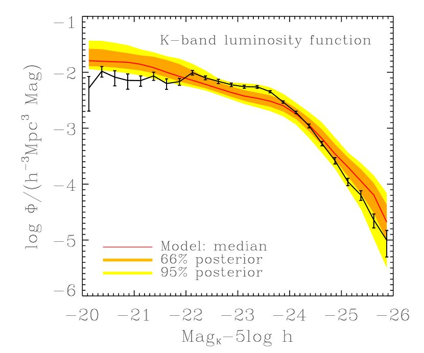
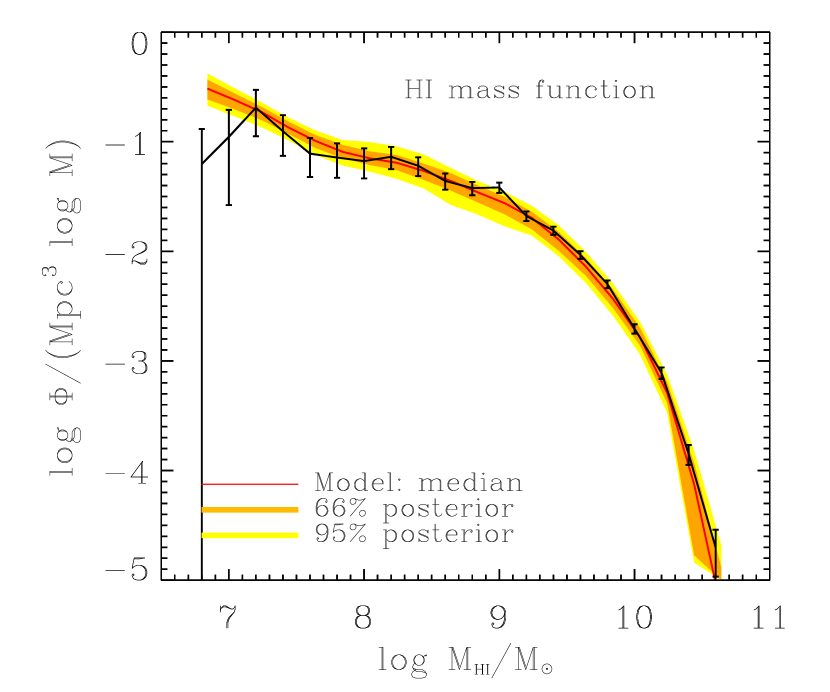
Figure 1: The Bayesian posterior predictions for the $K$-band luminosity function and the HI mass function. The black solid lines with error bars are the observational data. The orange and yellow bands encompass the 66% and 95% credible ranges of the predictions, respectively, while the red lines are the median values.

Figure 1 shows the posterior predictions for the $K$-band luminosity function and HI mass function of local galaxies. We account for potential incompleteness in the faint end of the $K$-band luminosity function by marginalising over the incompleteness parameter $\alpha_{\rm IN}$ (see Lu et al., 2012, for details). The orange and yellow bands in each panel encompass 66% and 95% of the posterior probability, respectively, and the red line is the median. To quantify the goodness of fit, we use posterior predictive check (PPC, Rubin, 1984; Gelman, Meng & Stern, 1996; Gelman et al., 2003). PPC compares the value of one or more discrepancy statistics for the observed data to a reference distribution based on the posterior (which is conditioned on the observed data). The reference distribution is obtained by generating predicted data from the posterior distribution. If a model fits the data well, the observed data should be likely under the posterior predictive distribution, and the discrepancy statistics of the observation should be likely under the distribution of the discrepancy statistics of the posterior models. On the other hand, large discrepancies between the observed data and the posterior predictive distribution indicate that the model performs poorly. Following our previous paper (Lu et al., 2012), we adopt the Bayesian $p$-value to quantify the goodness of fit, with $p$ defined as

$$p={1\over N}\sum_{i=1}^{N}I_{\chi_{i,{\rm mod}}^{2}\geq\chi_{\rm obs}^{2}}\,,$$ (27)

where $\chi_{i,{\rm mod}}^{2}$ and $\chi_{\rm obs}^{2}$ are the discrepancy statistics for the model and the data. $I_{q}$ is the indication function for the condition $q$, with $I_{q}=1$ if $q$ is true and $I_{q}=0$ otherwise. In other words, the fraction of posterior model samples with $\chi_{i,{\rm mod}}^{2}\geq\chi_{\rm obs}^{2}$ is an estimate of $p$. A small value of the $p$-value reflects the implausibility of the data under the model (and, hence, the lack of fit of the model to the data) and, therefore, suggests problems with the model. For the data and posterior distribution shown in Figure 1, the Bayesian $p$-value from the PPC for the HI mass function is $p_{\rm HI}=0.25$, which indicates an adequate fit, but for the $K$-band luminosity function it is only $p_{\rm K}=0.011$. This is much lower than the value of $p_{\rm K}=0.66$ obtained in Lu et al. (2012), which used only the $K$-band luminosity function as the data constraint. Hence, the model constrained using both the HI mass function and the $K$-band luminosity function does not fit the observational data well. In the remainder of this paper we will explore the causes for this discrepancy and their implication for models of galaxy formation generally.

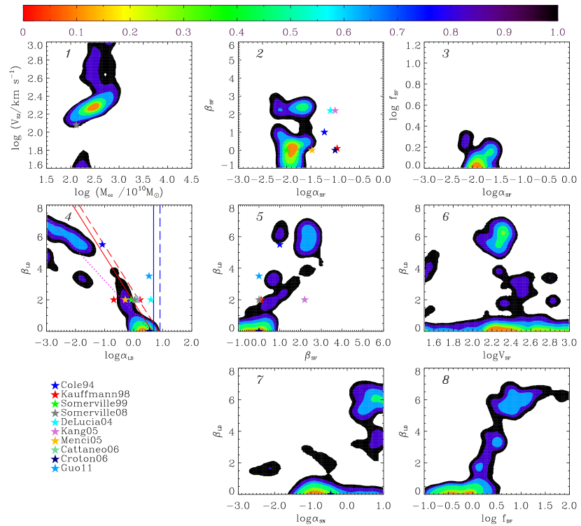
Figure 2: The marginalised posterior distributions of 10 model parameters. Panel 1: AGN feedback shuts off gas cooling for haloes with $M_{\rm vir}>M_{\rm CC}$ and winds expel gas from haloes with circular velocities $V_{\rm vir}>V_{\rm EJ}$. Panel 2: $\alpha_{\rm SF}$ parametrises the normalisation of star formation efficiency, which is a constant for haloes with a circular velocity higher than parameter $V_{\rm SF}$, and a power-law function of $V_{\rm vir}$ with $\beta_{\rm SF}$ being the power law index of the relation. Panel 3: $f_{\rm SF}$ is the cold gas surface density threshold for star formation and $\alpha_{\rm SF}$ is as above. Panel 4: $\alpha_{\rm LD}$ parametrises the loading factor of the SN feedback and $\beta_{\rm LD}$ is the power index of the power-law dependence of the loading factor on the halo circular velocity. The blue lines denote the kinetic energy limit based on Type II SN for outflows in haloes with a circular velocity of 220 km/s for two IMFs: Salpeter (solid) and Chabrier (dashed). The red lines show the extreme parameter combination of the two mass-loading parameters for haloes with a circular velocity of 100 km/s. Models in regions to the right of the limiting lines require more than 100% of the total available energy for the cold gas ejection. The magenta dotted line denotes models with a loading factor equal to 4 for haloes with a circular velocity of 70 km/s. Panel 5: the joint marginalised posterior distribution in the $\beta_{\rm LD}$-$\beta_{\rm SF}$ plane. Panel 6: the joint marginalised posterior distribution in the $\beta_{\rm LD}$-$V_{\rm SF}$ plane. Panel 7: $\alpha_{\rm SN}$ characterises the fraction of SN energy that is required to power the ejection of hot halo gas. Panel 8: the joint marginalised posterior distribution in the $\beta_{\rm LD}$-$\log f{\rm DF}$ plane, where $f_{\rm DF}$ is a coefficient characterising the satellite dynamical friction timescale. The greyscale (colour in on-line version) denotes the confidence levels as shown by the colour bar at the top of the figure. Symbols with different colours in the various panels denote the corresponding parameters adopted in some earlier SAMs, as indicated. They do not appear in every panel for all models because some parameters are absent in the parametrisation of those models.

Figure 2 shows marginalised posterior distributions for 10 parameters characterising star formation and feedback and we now describe those with marginal distributions that differ significantly from those in Lu et al. (2012). In the upper-left panel of Figure 2, the vertical axis shows the model parameter $V_{\rm EJ}$: the halo circular velocity below which all outflowing mass reheated from the disk must be ejected out of the host halo. The horizontal axis shows the parameter $M_{\rm CC}$: the critical halo mass above which radiative cooling of the halo gas is shut off to mimic radio-mode AGN feedback (Croton et al., 2006; Bower et al., 2006). The mass $M_{\rm CC}$ is well constrained, with a value about $10^{12.5}\>{\rm M_{\odot}}$. This result also agrees with the value obtained by Lu et al. (2012) using the $K$-band luminosity function alone as a data constraint, and with other existing SAMs that implement “halo quenching” (e.g. Cattaneo et al., 2006; Somerville et al., 2008). Including the HI mass function as an additional constraint does not affect the inferred value of $M_{\rm CC}$ significantly because $M_{\rm CC}$ controls gas cooling and star formation in massive haloes while the HI mass function mainly constrains low-mass haloes, which contain most of the HI gas.

The value of $V_{\rm EJ}$ is also well constrained, with $\log V_{\rm EJ}\approx 2.3$ ($V_{\rm EJ}\approx 200\,{\rm km/s}$), suggesting that all haloes with circular velocities lower than this are required to have efficient mass ejection to fit the data, and the same ejection process can be inefficient in haloes with higher circular velocities. There is also a non-negligible tail to even larger $V_{\rm EJ}$; models in this tail require efficient mass ejection at even higher halo circular velocities. This result agrees with both the model of Somerville et al. (2008) and a recent analysis of the Munich model (Henriques et al., 2013): efficient gas ejection from halos is required to match multiple data sets simultaneously. Without the HI constraint, the observed $K$-band luminosity function of galaxies can be reproduced by making the star formation efficiency a strong function of circular velocity, resulting in a massive cold-gas component. However, this makes the amplitude of the corresponding predicted HI mass function an order of magnitude higher than that observed (Lu et al., 2012; Wang, Weinmann & Neistein, 2012). In our model, the strong degeneracy between outflow and star formation efficiency is broken by the constraint provided by the HI mass function. Consequently, one requires efficient gas ejection from halos to prevent a large reservoir of cold gas and only requires the star formation efficiency to be a weak function of halo circular velocity (see below). If we fix $V_{\rm EJ}=0$, we find that the model can no longer match the observational data; the best fitting model, i.e. in this case the model with the maximum a posteriori (MAP) probability, has a likelihood that is almost 9,000,000 times lower than our fiducial MAP. This suggests that efficient gas ejection is unavoidable in our model family.

4.1.1 Star formation

With the HI mass function as an additional constraint, the posterior probability of the star formation parameters is now constrained to a fairly narrow range (see Panel 2 of Figure 2). The posterior of $\log(\alpha_{\rm SF})$ peaks sharply at $-1.8$, implying that a galaxy converts about $\approx 1.6\%$ of its cold gas into stars in every dynamical time. This is consistent with the observed efficiency in galaxies (Silk, 1997; Elmegreen, 1997). The posterior for $\beta_{\rm SF}$ is now peaked near zero, much lower than the value of $\beta_{\rm SF}\approx 10$ obtained in Lu et al. (2012) constrained using the $K$-band luminosity function alone. This low value for $\beta_{\rm SF}$ means that the star-formation rate is largely determined by the available supply of cold dense gas and does not depend on the mass (or circular velocity) of the host halo. This is consistent with observed star-formation laws (Schmidt, 1959; Kennicutt, 1989), in which the star formation rate depends only on gas properties. However, there still remains a weaker mode - its posterior odds relative to the main mode is 2.5 times smaller - where $\alpha_{\rm SF}\approx 2$% and $\beta_{\rm SF}\approx 2.5$. We will show that the parameter $\beta_{\rm SF}$ is covariant with feedback parameters in another panel of the figure.

In Lu et al. (2012), the star-formation efficiency parameter $\alpha_{\rm SF}$ was found to be strongly covariant with the threshold of cold gas surface density for star formation, $f_{\rm SF}$: a high star formation efficiency with a high threshold value was equivalent to a low star formation efficiency with a low threshold value. As expected, the addition of the HI mass function breaks this degeneracy. Panel 3 of Figure 2 shows the marginalised posterior probability distribution in the $\log f_{\rm SF}$–$\log\alpha_{\rm SF}$ plane. Remember that in our parametrisation, $f_{\rm SF}$ is equal to the surface gas density threshold for star formation, $\Sigma_{\rm SF}$, under the assumption that $r_{\rm disc}=r_{\rm disc,0}$, i.e. that the disc size is given by the model of Mo, Mao & White (1998). The combined data sets require that the threshold surface density for star formation is small; we find $\Sigma_{\rm SF}\approx 1\>{\rm M_{\odot}}{\rm pc}^{-2}$. This value is about one order of magnitude lower than the observed threshold surface density (Kennicutt, 1998; Bigiel et al., 2008; Leroy et al., 2008) and is also right against the prior bound, so even lower values may be preferred by the model, although such low values would be in even greater conflict with observations. In the model, a high gas surface density threshold would result in too much cold gas in low-mass haloes at large radii and too little star formation to power enough outflows. This problem was highlighted by Mo et al. (2005), who found that the standard threshold surface density for star formation would lead to an HI mass function that was too high, even if each low-mass halo only contained a cold gas disk at the threshold surface density.

Our SAM requires both powerful, efficient feedback to remove the gas from the halo and a threshold gas surface density that is much lower than the observed star formation threshold (and still fails to match the data). To explore explicitly the sensitivity to a higher surface density threshold, we constrained the prior of $f_{\rm SF}$ to range between $3\>{\rm M_{\odot}}\,{\rm pc}^{-2}$ and $30\>{\rm M_{\odot}}\,{\rm pc}^{-2}$. We find that this greatly reduces the goodness of fit and that the best fits are always obtained with $f_{\rm SF}$ at the lower boundary of the prior. The MAP using this restricted prior has a likelihood that is smaller than the MAP in the fiducial run by a factor of over 3,000,000. If we further restrict $f_{\rm SF}$ to match the observed value of $10\>{\rm M_{\odot}}\,{\rm pc}^{-2}$, the likelihood decreases by a further factor of over 60,000,000, and the $p$-value for the HI-mass function becomes very small, $p_{\rm HI}<0.005$, indicating an unacceptable fit. Thus, the current model family cannot explain the observed HI mass function using the observed gas density threshold for star formation.

4.1.2 Feedback

Panel 4 of Figure 2 shows the marginalised posterior probability distribution of the two supernova gas ejection parameters: $\alpha_{\rm LD}$ and $\beta_{\rm LD}$. For comparison, we also plot the combinations of these parameters used in a number of existing SAMs. These models include Cole et al. (1994), Kauffmann & Charlot (1998), Somerville & Primack (1999), Somerville et al. (2008), De Lucia, Kauffmann & White (2004), Kang et al. (2005), Menci et al. (2005), Cattaneo et al. (2006), and Guo et al. (2011). The parameter choices are converted into our parametrisation, where the amplitude of the mass-loading factor is normalised at a halo circular velocity scale of 220 km/s. As expected, because of the similarity in our phenomenological parametrisations, most of the other SAMs are located in the high probability region of our inferred posterior. These two parameters are covariant and populate three main modes: $\beta_{\rm LD}\approx 0$ that is equivalent to the Croton model (Croton et al., 2006), $\beta_{\rm LD}\approx 2$ that is similar to the Somerville model (Somerville et al., 2008) and a number of other models, and a large value of $\beta_{\rm LD}\approx 6$ (e.g. Cole et al., 1994).

Because we parametrise the outflow loading factor as a power-law function of halo circular velocity, $\alpha_{\rm ld}=\alpha_{\rm LD}(V_{\rm vir}/220{\rm km\,s^{-1}})^{-\beta_{\rm LD}}$, a covariance represented by a straight line in the $\log\alpha_{\rm LD}$–$\beta_{\rm LD}$ plane corresponds to a group of models that have a fixed loading factor for a specific circular velocity. The magenta dotted line in Panel 4 of Figure 2 roughly captures the covariance of the two parameters and corresponds to a loading factor of 4 for haloes with a circular velocity of $70{\rm km/s}$ or a mass of about $1.5\times 10^{11}\>{\rm M_{\odot}}$ at the present time. The covariance suggests that these haloes may be critical for fitting the $K$-band luminosity function and the HI mass function of galaxies simultaneously.

Our fiducial model does not limit the total energy available for feedback but, of course, Nature does impose limits. The total energy available for outflows powered by Type II supernovae is

$$E_{\rm SN,max}=\phi\eta_{\rm SN}\epsilon_{\rm SN}\,,$$ (28)

where $\epsilon_{\rm SN}\sim 10^{51}{\rm ergs}=5\times 10^{7}\>{\rm M_{\odot}}{\rm km^{2}\,s^{-2}}$ is the total energy output of a SN, and $\eta_{\rm SN}$ is the number of SNs expected from the formation of one solar mass of stars. Assuming that Type II SN progenitors are stars with masses $8\>{\rm M_{\odot}}<m<20\>{\rm M_{\odot}}$, then $\eta_{\rm SN}=5.88\times 10^{-3}\>{\rm M_{\odot}}^{-1}$ for a Salpeter IMF (Salpeter, 1955), and $\eta_{\rm SN}=9.76\times 10^{-3}\>{\rm M_{\odot}}^{-1}$ for a Chabrier IMF (Chabrier, 2003). The total energy consumed by the outflow depends on the detailed processes and the final state of the outflow material. If the outflow is thermalised and settles into an equilibrium state in the gravitational potential of the host halo, the energy required is ${5\over 4}m_{\rm rh}V_{\rm vir}^{2}$, where $m_{\rm rh}$ is the mass of the reheated gas (e.g. Kauffmann & Charlot, 1998). Since only a fraction of the energy is expected to heat the gas:

$$\eta_{\rm SN}\epsilon_{\rm SN}\geq{5\over 4}\alpha_{\rm LD}\left({220{\rm km/s}\over V_{\rm vir}}\right)^{\beta_{\rm LD}}V_{\rm vir}^{2}.$$ (29)

Thus, for haloes with $V_{\rm vir}=220\,{\rm km/s}$, the maximum normalisation of the loading factor, $\alpha_{\rm LD,max}(V_{\rm vir}=220)=4.13\times{\eta_{\rm SN}\over 5\times 10^{-3}}$, which is 4.8 for a Salpeter IMF and 8.0 for a Chabrier IMF. These values are plotted in the lower-right panel of Figure 2 as the blue solid line and the blue dashed line, respectively.

If the outflow is ejected directly from the centre of the host halo, the energy required to escape is ${1\over 2}m_{\rm ej}V_{\rm esc}^{2}$, where $V_{\rm esc}$ is the escape velocity. For a NFW halo (Navarro, Frenk & White, 1996) with a concentration $c=10$, the escape velocity from the centre is $V_{\rm esc}^{2}\approx 13\times V_{\rm vir}^{2}$. Thus, to eject the gas from such a halo, the lower limit on the required energy is $E={13\over 2}m_{\rm LD}V_{\rm vir}^{2}$, where $m_{\rm LD}$ is the total gas mass loaded in the wind. The mass-loading factor in such haloes is, therefore, limited by the total energy provided by SN explosions, and the solid red line and the red dashed line in Panel 4 of Figure 2 show these limits for a Salpeter and a Chabrier IMF, respectively. Models lying above such a limiting line need more energy than is available from haloes with circular velocities equal to or below 100 km/s. The posterior contours for all the modes with $\beta<4$ are $\sim 0.3-0.6$ dex to the left of but not far from the energy limits for haloes with $V_{\rm vir}\leq 100\,{\rm km/s}$, indicating that a large fraction, i.e. 25–50%, of all the supernova energy has to be put into the outflow in such galaxies.

The required high loading factor results from the need to simultaneously match the shallow low-end slope of both the $K$-band luminosity function and the HI mass function. The total baryonic mass that can be accreted into a halo is $f_{\rm b}m_{\rm vir}$, where $f_{\rm b}$ is the universal baryon fraction. Suppose a fraction $f_{\rm c}$ of the gas can cool and collapse onto the central galaxy. For low mass haloes with $V_{\rm vir}\la 150$ km/s, $f_{\rm c}$ is expected to be close to unity because of the high cooling efficiency (Thoul & Weinberg, 1995; Lu & Mo, 2007). If the expelled gas can fall back onto the galaxy and go through multiple cycles, the effective $f_{\rm c}$ can be larger than 1. However, to explain the shallow low-mass end of the HI mass function and the faint end slope of the $K$-band luminosity function, the cold gas and stellar mass has to be very low relative to $f_{\rm b}m_{\rm vir}$. Indeed, the stellar mass to halo mass ratio for haloes with masses $\sim 10^{11}\>{\rm M_{\odot}}$ is only about $3\times 10^{-3}$ (Yang et al., 2012; Papastergis et al., 2012; Behroozi, Wechsler & Conroy, 2013), and the cold gas mass to stellar mass ratio is no more than 10 (Kannappan, 2004; Papastergis et al., 2012). Thus, the gas associated with low-mass haloes either is never accreted into the galaxy or has been expelled by galactic winds. In the latter case, if we conservatively assume that the cold gas mass is 10 times the stellar mass, then the total cold baryonic mass in a $10^{11}\>{\rm M_{\odot}}$ halo is $\sim 0.033$ of the halo mass. If we make the further conservative assumption that for every unit of stellar mass formed at early times only half of it remains in stars today owing to stellar mass loss, the total mass that was ever involved in star formation is $\sim 0.006$ of the final halo mass. Based on these conservative assumptions, one finds that the mass-loading factor is $(f_{\rm b}-0.033)/0.006=23$, which is close to the upper limit obtained from the total kinetic energy expected from SN.

The posterior marginals (Fig. 2) imply that 25–50% of the available SN energy, depending on the assumed IMF, is required to power the wind. This required high efficiency of energy loading poses a severe challenge for the standard SN feedback scenario (e.g. Dekel & Silk, 1986; White & Zaritsky, 1992). Indeed, detailed hydrodynamical simulations by Mac Low & Ferrara (1999) and Strickland & Stevens (2000) demonstrated that supernova feedback is very inefficient in expelling mass because the onset of Rayleigh-Taylor instabilities severely limits the mass-loading efficiency of galactic winds. There are a couple of possible solutions to this dilemma. First, a top-heavy or bottom-light IMF would yield a larger $\eta_{\rm SN}$. Our data constraints are from the local galaxy population, which by themselves do not distinguish different IMFs. Second, the UV photons from massive stars could effectively transfer radiation momenta to the gas via dust opacity, thereby producing momentum driven winds (Murray, Quataert & Thompson, 2005). The total radiation energy available is about 100 times as high as the kinetic energy of supernova explosions, vitiating the mechanical energy limit. The viability of this mechanism is uncertain: while some simulations show that it is effective (e.g. Hopkins, Quataert & Murray, 2011), others find that the development of Rayleigh-Taylor type instabilities can suppress the formation of outflows (Krumholz & Thompson, 2012). Thus, although the required high efficiency may rule out mechanisms based on SN energy-driven winds alone, the viability including momentum-driven winds is still unclear.

The star formation feedback models implemented in SAMs are crude. In our model, the outflow reduces the total cold gas mass of the galaxy and the remaining cold gas is redistributed in an exponential profile at each time step. This is similar to some cosmological hydrodynamical simulations (e.g. Davé et al., 2013) where the effective viscosity of the disk gas, which could include actual gas viscosity and/or gravitational torques, causes the cold gas from the outer disk to move rapidly inwards to replenish the star forming gas, and so star formation can continue near the disk centre even if the total amount of gas in the disk is reduced. However, since the gas viscosity in such simulations is artificial and the resolution is still limited, it is unclear whether the effect is physical or numerical. For example, if the effective viscosity of the disk gas were unimportant, much of the cold gas would stay in the outer region of the disk without forming stars. Some simulations of individual disks (Forbes, Krumholz & Burkert, 2012) do find that star formation feedback is localised to regions where the star formation is active, producing a disk with a reduced cold gas density only in the central part of the disk, leaving the cold gas in the outskirts intact. Others confirm the cosmological simulation results (e.g. Hirschmann et al., 2013). To explore this in our SAM, we have considered a model in which star formation feedback is assumed to only affect the gas within the radius where star formation can happen, i.e. the cold density is above the threshold surface density. Without a lower limit on $f_{\rm SF}$, the posterior distribution is nearly unchanged owing to the low surface density threshold for star formation and the high outflow rate required by the shallow low-mass end of the galaxy luminosity function. However, if the value of $f_{\rm SF}$ is forced to match the observed star formation threshold surface density of $10\>{\rm M_{\odot}}\,{\rm pc}^{-2}$ then the model fails to fit the data ($p_{\rm HI}<0.005$), consistent with the results obtained by Mo et al. (2005).

As we remarked before, we find that there are three major modes in the $\log\alpha_{\rm LD}$–$\beta_{\rm LD}$ plane located at $\beta_{\rm LD}\approx$ 0, 2, and 6, as one can see in Panel 4 of Figure 2. The relative posterior odds in each mode are 4:1:2, respectively. Hence, the $\beta=0$ mode is favoured by the combined data sets in terms of marginalised posterior probability. Since our prior distribution is intentionally very broad, as we describe in §2, and this will quantitatively affect these odds. That said, the maximum likelihood is located in the $\beta_{\rm LD}\approx 6$ mode, and the highest likelihood values in the $\beta_{\rm LD}\approx 2$ and 0 modes are 30 and 1,400 times lower, indicating that those two modes produce a worse fit to the data than the $\beta_{\rm LD}\approx 6$ mode. The PPC $p$-values calculated for the $K$-band luminosity function predicted by each of the modes also indicate that the $\beta_{\rm LD}\approx 6$ mode produces a better, but still inadequate, fit to the data, $p_{\rm K}=0.016$ for the $\beta_{\rm LD}\approx 6$ mode, and $p_{\rm K}<0.005$ for the other two modes. In Figure 3, we show the $K$-band luminosity function produced by the three modes. The shaded blue region shows the posterior predictions of models with $\beta_{\rm LD}<1.25$, the magenta region shows the posterior predictions of models with $1.25<\beta_{\rm LD}<4$, and the green region shows the posterior predictions of models with $\beta_{\rm LD}>4$. Note that the three modes produce indistinguishable predictions for the HI mass function, as the predictive distribution of the HI mass function produced by the entire posterior shown in Figure 1 is narrow. The predicted faint-end slope of the $K$-band luminosity function is steeper for a smaller value of $\beta_{\rm LD}$, and the current data apparently favours the mode with the highest $\beta_{\rm LD}$. This trend confirms recent hydro-dynamical simulation results of Puchwein & Springel (2013) and Davé et al. (2013). Moreover, this demonstrates that discrimination between these modes could be possible given improved data for the faint end of the luminosity function.

Even though the $\beta_{\rm LD}\approx 0$ mode has relatively lower likelihood, it has the highest marginal posterior probability. This implies that the modes with high values of $\beta_{\rm LD}$ are supported by proportionately smaller volumes in parameter space relative to the $\beta_{\rm LD}\approx 0$ mode. This could be investigated in detail using the distribution of marginal likelihood, but the required resolution to compute the volume in the high-dimensional parameter space is computationally prohibitive. Nonetheless, relying on the posterior marginals shown in Figure 2, we believe that the complex posterior results from the fine tuning necessary to simultaneously match the $K$-band luminosity and HI mass function. Specifically, Panel 5 indicates that $\beta_{\rm SF}$ correlates with $\beta_{\rm LD}$. As $\beta_{\rm SF}$ increases, the increasingly smaller star formation efficiency in low circular velocity haloes leaves more cold gas in the disk. To simultaneously match the HI mass function, the model thus needs to increase the feedback efficiency in lower circular velocity halos by increasing $\beta_{\rm LD}$.

In addition, sometimes a particular parametrisation can also introduce specific features into the posterior. Panel 6 of Fig. 2 shows an example; the parameter $V_{\rm SF}$ is not constrained when $\beta_{\rm LD}\approx 0$, but is strongly constrained when $\beta_{\rm LD}\approx 6$. When $\beta_{\rm LD}\approx 0$, $\beta_{\rm SF}$ is also about 0, meaning a constant star formation efficiency. In this case, as described in §2, $V_{\rm SF}$ no longer has any effect on the model predictions, because the parametrisation for the star formation efficiency no longer has a transition scale that $V_{\rm SF}$ describes. Thus, the likelihood is the same no matter what value $V_{\rm SF}$ takes when $\beta_{\rm LD}\approx 0$.

Moreover, the high $\beta_{\rm LD}$ mode requires two unusual conditions. First, as shown in Panel 7 of Fig. 2, for $\beta_{\rm LD}\approx 6$, the parameter $\alpha_{\rm SN}$, which characterises the fraction of SN kinetic energy used to eject the hot halo gas, is always required to be higher than one, implying that the required energy is higher than the kinetic energy provided by SN Type II. The reason is that $\beta_{\rm LD}\approx 6$ leads to a rapid decrease of cold gas ejection with increasing halo circular velocity, and a strong outflow of hot halo gas in relatively massive halos is needed by the mode to fit the data. This conclusion agrees with the result of Mutch, Poole & Croton (2013) that one needs more energy than that available from SN Type II to explain the evolution of the galaxy stellar mass function from $z\approx 0.8$ to 0. Second, the $\beta_{\rm LD}\approx 6$ mode also requires a long time scale, about 10 times as long as the fiducial dynamical friction timescale, for satellite galaxies to orbit in the host halo before merging into central galaxies (see Panel 8 of Fig. 2). This can be understood as follows. When $\beta_{\rm LD}$ is large, the effect of star formation feedback is increasingly weaker for higher mass haloes. In this case, the merging timescale for satellite galaxies is required to be long to prevent them from merging into the halo centre and hence significantly increasing the mass of the central galaxy. Since a longer merger time also leads to a higher satellite fraction, observational data of satellite fraction can tighten the constraint. We will come back to this topic in a future paper.

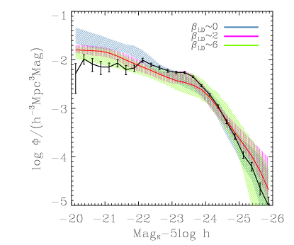
Figure 3: The predicted $K$-band luminosity function for the three different modes present in the lower-right panel of Fig. 2 represented by different values of $\beta_{\rm LD}$. The red line is the median prediction for the entire posterior.

4.2 Posterior Predictions

The model family generally requires efficient outflows from low-mass galaxies for its best fit, but even that is not enough to match both of the constraining observational data sets. We now use the posterior distribution to predict the outflow rate and other observables to investigate the failure of the model family. Since the marginalised posterior in the $\alpha_{\rm LD}$–$\beta_{\rm LD}$ plane is multi-modal, we distinguish the modes according to their value of $\beta_{\rm LD}$ when making model predictions. We marginalise the posterior probability to generate predictions as described in Lu et al. (2012).

Figure 4 shows the posterior prediction for the cold baryonic mass fraction (cold gas plus stars) of central galaxies normalised by the cosmic baryon fraction, $f_{\rm b}$, as a function of halo mass. The red line shows the median of the whole posterior prediction, while the shaded regions with different colours encompass the 95% credible ranges from the modes with $\beta_{\rm LD}\sim 0$, 2, and 6, as indicated in the figure. The black bars show the results of abundance matching obtained by Papastergis et al. (2012) using the ALFALFA and SDSS data.

The observed $K$-band luminosity function only determines absolute magnitudes up to $K={\rm Mag_{K}}-5\log h=-20$, which only constrains the halo virial mass above $\sim 10^{11}\>{\rm M_{\odot}}$ (indicated as the vertical line in Fig. 4). The 95% range of the posterior prediction contains the abundance matching result for haloes more massive than a few times $10^{11}\>{\rm M_{\odot}}$, but all three modes overpredict the cold baryon fraction for lower mass haloes. Among the three modes, models with larger $\beta_{\rm LD}$ produce lower cold baryon mass fractions for low mass haloes. The mode with $\beta_{\rm LD}\approx 0$ vastly overpredicts the cold baryon mass fraction in haloes with masses $\leq 10^{11.5}\>{\rm M_{\odot}}$.

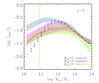
Figure 4: The posterior predictive distribution of the cold baryon (stars plus cold gas) mass fraction as a function of halo mass. The shaded bands with different colours encompass the 95% credible range of the prediction for the three modes represented by different values of $\beta_{\rm LD}$, while the red line is the predicted median of the entire posterior predictive distribution. The black points with error bars are from Papastergis et al. (2012). The vertical yellow dashed line marks the lowest halo mass constrained by the $K$-band luminosity function.

To explore the physical implications of feedback, we predicted the average star formation rate (SFR) and outflow rate (OFR) in each mass bin for all central galaxies at $z=0$. Figure 5 shows the ratio OFR/SFR, which is commonly referred to as the mass-loading factor of the wind. Again the red lines show the medians of the whole posterior prediction, while the shaded regions with different colours encompass the 95% credible range from the three modes defined by their values of $\beta_{\rm LD}$. The predicted OFR/SFR ratio generally decreases with stellar mass; it is approximately 10 for galaxies with stellar masses $\la 10^{8.5}\>{\rm M_{\odot}}$ and close to 1 for Milky-Way mass galaxies. Observationally, there is no strong evidence for the existence of such a strong stellar mass dependence for outflows in normal disk galaxies at the present day (see Heckman, 2003; Veilleux, Cecil & Bland-Hawthorn, 2005; Rupke, Veilleux & Sanders, 2002; Martin, 2006). In starburst galaxies, the mass outflow rates are roughly comparable to the star-formation rate, so that OFR/SFR $\sim 1$, and lower mass galaxies do not show stronger outflows. Thus, the high OFR/SFR ratio predicted for the general dwarf galaxy population does not have any observational support, but then again there is no strong observational evidence against it. Comparing the predictions for the different posterior modes, we see that different choices of $\beta_{\rm LD}$ produce very different trends of the loading factor with galaxy stellar mass. The $\beta_{\rm LD}\approx 0$ mode produces a constant mass-loading factor, ${\rm OFR/SFR}\approx 3$ over a large stellar mass range, while the other two modes predict a rapidly decreasing ${\rm OFR/SFR}$ with increasing stellar mass. The roughly constant ${\rm OFR/SFR}$ predicted by the $\beta_{\rm LD}\sim 0$ mode is consistent with the observational results of Martin (2006), but this mode significantly overpredicts the cold baryon mass fraction for low mass haloes. Clearly, as one needs a large mass-loading factor to achieve better fits to the constraining data, observations of gas outflows in low-mass galaxies and how they scale with galaxy mass can provide important constraints on the feedback model family considered here.

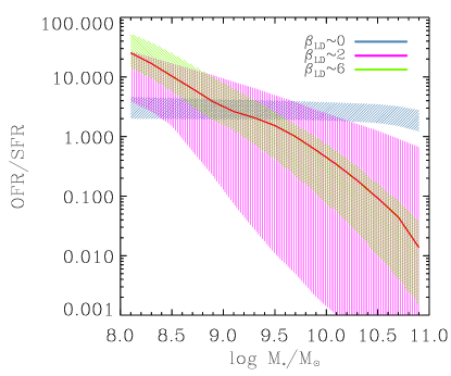
Figure 5: The predicted ratio of mass outflow rate to star formation rate as a function of stellar mass for central galaxies at $z=0$. The colour bands and lines are as described in Fig. 4.

Figure 6 shows the predicted cosmic star formation rate density as a function of redshift using the posterior samples selected from the three modes of $\beta_{\rm LD}$. The grey shaded region in the figure denotes a compilation of observational estimates of the cosmic star formation rate density as a function of redshift from Behroozi, Wechsler & Conroy (2013). Compared to the data, our model family predicts a different shape. The cosmic star formation rate density in the model reaches its maximum at higher redshifts ($z\approx 3.5$), while data suggests it more sharply peaks around $z\approx 2$, although the observed drop at high redshifts could partly owe to missing low mass galaxies (Lu et al., 2014). The model also underpredicts the star formation rate density around $z=2$, as the median of the posterior predictive distribution is only marginally enclosed by the lower bound of the observational data. The predictions from the $\beta_{\rm LD}\approx 0$ mode are systematically higher and might be more consistent with the observations. The high $\beta_{\rm LD}$ mode predicts a star formation rate density that is too low to match the observational data at $z>1$. This stems from the powerful SN driven outflows in low-mass haloes required to fit the local galaxy luminosity function and HI mass function. Because the parametrisation for feedback does not have an explicit redshift dependence, such strong outflows work throughout all cosmic time in the model. This feedback suppresses star formation at high redshift where such low-mass haloes dominate.

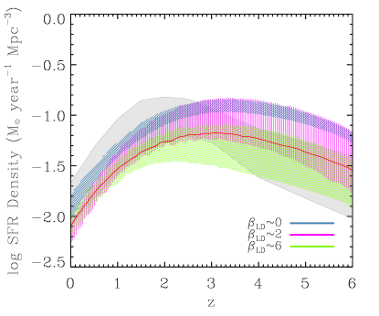
Figure 6: The posterior prediction of the co-moving star formation rate density versus redshift. Points with error bars are observational data. The grey band denotes observational estimates compiled in Behroozi et al. 2013. The other colour bands and lines are as described in Fig. 4.

Figure 7 shows the star formation rate (SFR) as a function of redshift for haloes with masses of $M_{\rm vir}=10^{12}\>{\rm M_{\odot}}$ today ($z=0$) for the three modes in $\beta_{\rm LD}$. The model predictions are compared with the recent results obtained by Lu et al. (2014) and Behroozi, Wechsler & Conroy (2013) using empirical models tuned to fit the observed stellar mass functions at different redshifts. The empirical models predict a peak near $z\approx 1$ while our SAM family predicts a much weaker peak at higher $z$. This is consistent with the underprediction of the SFR density at $z\approx 1$ in Figure 6. The $\beta_{\rm LD}=0$ mode also overpredicts the SFR at $z>2$, although this mode better matches the observed cold gas fraction in haloes with masses of $10^{12}{\rm M}_{\odot}$ (see Figure 4). Overall, the predicted star formation histories for Milky Way sized galaxies by our SAM family are inconsistent with the results obtained from the empirical models.

Figure 7: The posterior prediction of the star-formation-rate history for haloes with present-day mass $10^{12}{\rm M}_{\odot}$. Points with error bars show results obtained with two recent empirical models. The colour bands and lines are as described in Fig. 4.

Weinmann et al. (2012) found that SAMs and numerical simulations cannot generally reproduce the observed number density evolution of low mass galaxies. For comparison, we predict the number densities of galaxies with stellar masses in the range $9.27\leq\log M_{*}/\>{\rm M_{\odot}}\leq 9.77$ from $z=0$ to 6, and compare them with the observational data compiled by Weinmann et al. (2012). Figure 8 shows that the model family can accommodate the observational data at $z=0$, but vastly overpredicts the number density of low-mass galaxies at higher redshift. This confirms the results of Weinmann et al. (2012), and suggests that the current model family cannot match the data even if a large parameter space is explored.

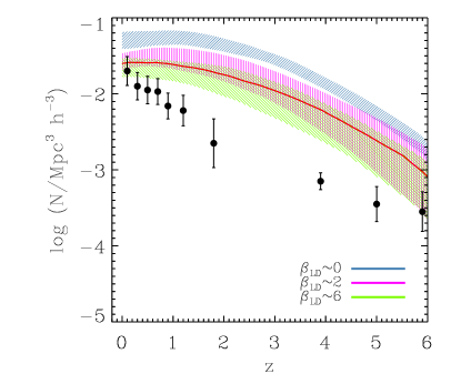
Figure 8: The posterior prediction for the evolution of the number density of galaxies with stellar masses in the range $\log(M_{*}/\>{\rm M_{\odot}})=9.27-9.77$ as a function of redshift. Points with error bars show data compiled by Weinmann et al. (2012). The colour bands and lines are as described in Fig. 4.

Figure 9 shows the prediction of the co-moving mass density of cold gas as a function of redshift. The observational data at high redshifts, estimated using damped Lyman alpha systems (Péroux et al., 2003; Prochaska & Wolfe, 2009), suggests that the cold gas density at high redshifts is higher than in the local universe. Our predicted increase of the cold gas mass density with redshift in the range from $z=0$ to 2 is consistent with the observations. The model also predicts a decrease of the cold gas density with increasing redshift at $z>3$. Unfortunately the current data is still too uncertain to provide meaningful constraints on the model.

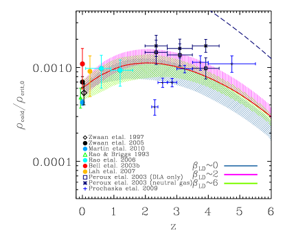
Figure 9: The posterior prediction for the co-moving cold gas mass density normalised by the critical density of the universe at the present time. The blue dashed line shows the total mass in haloes with $m_{\rm vir}\geq 5\times 10^{9}\>h^{-1}\rm M_{\odot}$ times the universal baryon fraction $f_{\rm b}$. Points with error bars are observational data from Zwaan et al. (1997, 2005); Martin et al. (2010); Rao & Briggs (1993); Rao, Turnshek & Nestor (2006); Lah et al. (2007); Péroux et al. (2003) and Prochaska & Wolfe (2009). The colour bands and lines are as described in Fig. 4.

In summary, the model family considered here, which has physical prescriptions similar to most published SAMs, in addition to not fitting one of the constraining data sets, the observed $K$-band luminosity function, also fails to predict additional observations as follows:

1. It requires very efficient feedback to eject gas from low-mass haloes. The energy required is probably too high if the outflows are driven by the kinetic energy of supernova explosions alone, although this problem may be alleviated by including radiation pressure.

2. It requires a density threshold for star formation that is much lower than current observations suggest, owing to the energy needed to eject cold gas from the disk.

3. The high mass-loading factor required by the present-day distribution of low-mass galaxies predicts mass outflow rates that might be too high to match observation.

4. The predicted star formation rate history of Milky-Way-sized galaxies is inconsistent with that obtained from empirical models.

5. It overpredicts the number density of low-mass galaxies at high redshift.

These results together suggest that some important physics may still be missing in the current SAMs.

5 Discussion and conclusions

We use the observed low redshift $K$-band luminosity function and HI-gas mass function of galaxies as data constraints to explore star-formation and feedback in a semi-analytic model of galaxy formation, which uses MCMC-based Bayesian methodology. The combination of these two data sets breaks the degeneracy in the parametrised phenomenology based on using the $K$-band luminosity function data constraint alone (Lu et al., 2012). Our model assumes that baryons accrete into the assembling halo where they cool, form stars, and the resulting feedback ejects some fraction of the gas. Our model has many features in common with most published SAMs and our results focus on conclusions generic to a large class of published models. We marginalise over all the uncertainties in the model family that are not constrained by the data sets.

Our broad parameter space covers and extends the ranges of the important parameters for star formation and feedback adopted in many existing SAMs. Our exhaustive parameter-space search results in the robust identification of several compact modes that best match the constraining data. These modes are likelihood dominated, i.e. the existence of these modes does not depend sensitively on the prior distribution as long as the modes are supported. The analyses presented in this paper focus on the behaviour of the model constrained to those modes, namely on the physical implications of the constrained parameters and the predictions of these modes. These conclusions are not expected to depend sensitively on the prior. However, the choice of the prior distribution is generally important in complex high dimensional problems, especially when the likelihood is not sufficiently informative. In such cases, strong prior belief easily sways weak observational constraints. Conversely, a thorough investigation of the poorly constrained model motivates the acquisition of data that robustly discriminates between competing hypotheses of interest.

Overall, our model fails to reproduce the joint data sets and, therefore, more work will be required to understand the nature of the failure and to propose a remedy before attempting a quantitative Bayesian analysis. To assess the fit, we use the posterior predictive check (PPC) method with a residual sum of squares for each bin, for both the $K$-band luminosity function and the HI-gas mass function, as a discrepancy statistic. In this method, the discrepancy with the data is compared with the distribution predicted from the posterior distribution. We find that the data is in the tail of the distribution defined by the posterior, suggesting the implausibility of the data given the model.

The primary cause for the failure is that to simultaneously produce the observed stellar component and the observed cold gas fraction at the low mass end requires the SN feedback to be extremely efficient in expelling gas. This requires a high mass-loading factor that consumes much of the available energy budget. The low $p$-value we found by exhaustively exploring the parameter space has its roots in the over simplicity of the phenomenological model and suggests that key physical processes are missing or misrepresented.

In addition, we find that the mass-loading factor must depend strongly on halo circular velocity to obtain the shallow faint-end slope of the luminosity function. The model requires that winds from haloes with circular velocities lower than $\sim 200{\rm km\,s^{-1}}$ are ejected from the halo, completely. However, in many mass-loading models the mass-loading factor is a weak function of the halo circular velocity. Recent simulations concur: Davé et al. (2013) show that a steeper relation between mass-loading and halo circular velocity tends to produce a shallower stellar and HI mass function at the low-mass end. This also suggests that accurate observational data for the faint-end slope of the galaxy luminosity function are crucial to constrain feedback models.

The inferred requirement for efficient feedback is consistent with the recent results of Mutch, Poole & Croton (2013) and Henriques et al. (2013) who also found that a high efficiency of SN feedback is needed to fit the stellar mass and/or luminosity functions of galaxies at multiple redshifts. However, the high efficiency implied by the posterior distribution obtained here is not supported by hydro-dynamical simulations (e.g. Mac Low & Ferrara, 1999), which showed that the feedback efficiency of SN kinetic energy is usually quite low. Thus, either some other important energy sources are missing or the way feedback works is not correctly modelled in the current model family. For example, radiation pressure associated with star formation and SN explosions may provide a viable solution to the energy problem found here (e.g. Stinson et al., 2013).

Finally, the model predicts the star formation history over all time, although it is only constrained by data at $z=0$. The observed star formation histories of Milky Way-sized haloes and the observed redshift evolution in the number density of low-mass galaxies at high $z$ are inconsistent with our posterior predictions. This suggests that star formation and feedback may have a more complex redshift dependence than assumed here.

In summary, our analysis shows that we require a high wind mass loading factor and mass ejection rate of galactic winds to match the observed luminosity and cold gas mass functions. This result applies to many if not all ejective feedback scenarios that depend on winds, largely independent of the mechanistic details. This is a direct consequence of a short radiative cooling time scale in low-mass haloes combined with the small fraction of baryons in stars and cold gas relative to the cosmic baryon fraction. Moreover, the predicted high mass-loading factor and mass-loss rates are not observed, suggesting that a feedback-generated wind may not be the agent suppressing star formation and cold gas accretion in low-mass haloes, at least at low-$z$.

Alternatively, this suggests exploring mechanisms that prevent the gas accretion in the first place. For example, the intergalactic medium (IGM) may be preheated by some processes so that low mass haloes can accrete baryonic matter only at a reduced rate, either by properly including the effects of already considered processes like supernova winds or by additional processes like gravitational pancaking or Blazar heating (e.g. Mo & Mao, 2002; Mo et al., 2005; Lu & Mo, 2007; Anderson & Bregman, 2010; Zhu, Feng & Fang, 2011; Pfrommer, Chang & Broderick, 2012). This may also introduce a characteristic time before and after which the star formation and feedback proceed differently, as seems to be required to match the star formation history and number density evolution of low mass galaxies (see Lu et al., 2014). We will investigate the effects of preheating on galaxy formation in a future paper.

References

- Anderson & Bregman (2010) Anderson M. E., Bregman J. N., 2010, ApJ, 714, 320
- Behroozi, Wechsler & Conroy (2013) Behroozi P. S., Wechsler R. H., Conroy C., 2013, ApJ, 770, 57
- Bell et al. (2003a) Bell E. F., McIntosh D. H., Katz N., Weinberg M. D., 2003a, ApJ, 585, L117
- Bell et al. (2003b) Bell E. F., McIntosh D. H., Katz N., Weinberg M. D., 2003b, ApJS, 149, 289
- Benson et al. (2003) Benson A. J., Bower R. G., Frenk C. S., Lacey C. G., Baugh C. M., Cole S., 2003, ApJ, 599, 38
- Bigiel et al. (2008) Bigiel F., Leroy A., Walter F., Brinks E., De Blok W. J. G., Madore B., Thornley M. D., 2008, AJ, 136, 2846
- Bower, Benson & Crain (2012) Bower R. G., Benson A. J., Crain R. A., 2012, MNRAS, 422, 2816
- Bower et al. (2006) Bower R. G., Benson A. J., Malbon R., Helly J. C., Frenk C. S., Baugh C. M., Cole S., Lacey C. G., 2006, MNRAS, 370, 645
- Bower et al. (2010) Bower R. G., Vernon I., Goldstein M., Benson A. J., Lacey C. G., Baugh C. M., Cole S., Frenk C. S., 2010, MNRAS, 407, 2017
- Bruzual (2007) Bruzual G., 2007, in Astronomical Society of the Pacific Conference Series, Vol. 374, From Stars to Galaxies: Building the Pieces to Build Up the Universe, A. Vallenari, R. Tantalo, L. Portinari, & A. Moretti, ed., pp. 303–+
- Cattaneo et al. (2006) Cattaneo A., Dekel A., Devriendt J., Guiderdoni B., Blaizot J., 2006, MNRAS, 370, 1651
- Chabrier (2003) Chabrier G., 2003, PASP, 115, 763
- Chen et al. (2010) Chen Y.-M., Tremonti C. A., Heckman T. M., Kauffmann G., Weiner B. J., Brinchmann J., Wang J., 2010, AJ, 140, 445
- Cole et al. (1994) Cole S., Aragón-Salamanca A., Frenk C. S., Navarro J. F., Zepf S. E., 1994, MNRAS, 271, 781
- Croton et al. (2006) Croton D. J. et al., 2006, MNRAS, 365, 11
- Davé et al. (2013) Davé R., Katz N., Oppenheimer B. D., Kollmeier J. A., Weinberg D. H., 2013, MNRAS, 434, 2645
- De Lucia & Blaizot (2007) De Lucia G., Blaizot J., 2007, MNRAS, 375, 2
- De Lucia, Kauffmann & White (2004) De Lucia G., Kauffmann G., White S. D. M., 2004, MNRAS, 349, 1101
- Dekel & Silk (1986) Dekel A., Silk J., 1986, ApJ, 303, 39
- Dunkley et al. (2009) Dunkley J. et al., 2009, ApJS, 180, 306
- Elmegreen (1997) Elmegreen B. G., 1997, ApJ, 486, 944
- Forbes, Krumholz & Burkert (2012) Forbes J., Krumholz M., Burkert A., 2012, ApJ, 754, 48
- Gelman et al. (2003) Gelman A., Carlin J. B., Stern H. S., Rubin D. B., 2003, Bayesian Data Analysis, 2nd edn., Texts in Statistical Science. CRC Press, Boca Raton, FL
- Gelman, Meng & Stern (1996) Gelman A., Meng X.-L., Stern H., 1996, Statistica Sinica, 6, 733
- Gelman & Rubin (1992) Gelman A., Rubin D., 1992, Statistical Science, 7, 457
- Giovanelli et al. (2005) Giovanelli R. et al., 2005, AJ, 130, 2598
- Gómez et al. (2012) Gómez F. A., Coleman-Smith C. E., O’Shea B. W., Tumlinson J., Wolpert R. L., 2012, ApJ, 760, 112
- Guo et al. (2011) Guo Q. et al., 2011, MNRAS, 413, 101
- Heckman (2003) Heckman T. M., 2003, in Revista Mexicana de Astronomia y Astrofisica, vol. 27, Vol. 17, Revista Mexicana de Astronomia y Astrofisica Conference Series, Avila-Reese V., Firmani C., Frenk C. S., Allen C., eds., pp. 47–55
- Henriques et al. (2009) Henriques B. M. B., Thomas P. A., Oliver S., Roseboom I., 2009, MNRAS, 396, 535
- Henriques et al. (2013) Henriques B. M. B., White S. D. M., Thomas P. A., Angulo R. E., Guo Q., Lemson G., Springel V., 2013, MNRAS, 431, 3373
- Hirschmann et al. (2013) Hirschmann M. et al., 2013, MNRAS, 436, 2929
- Hopkins et al. (2013) Hopkins P. F., Cox T. J., Hernquist L., Narayanan D., Hayward C. C., Murray N., 2013, MNRAS, 430, 1901
- Hopkins, Quataert & Murray (2011) Hopkins P. F., Quataert E., Murray N., 2011, MNRAS, 417, 950
- Kampakoglou, Trotta & Silk (2008) Kampakoglou M., Trotta R., Silk J., 2008, MNRAS, 384, 1414
- Kang et al. (2005) Kang X., Jing Y. P., Mo H. J., Börner G., 2005, ApJ, 631, 21
- Kannappan (2004) Kannappan S. J., 2004, ApJ, 611, L89
- Kauffmann & Charlot (1998) Kauffmann G., Charlot S., 1998, MNRAS, 294, 705
- Kennicutt (1989) Kennicutt J. R. C., 1989, ApJ, 344, 685
- Kennicutt (1998) Kennicutt, Jr. R. C., 1998, ARA&A, 36, 189
- Kennicutt et al. (2007) Kennicutt R. C. J. et al., 2007, ApJ, 671, 333
- Keres, Yun & Young (2003) Keres D., Yun M. S., Young J. S., 2003, ApJ, 582, 659
- Komatsu et al. (2009) Komatsu E. et al., 2009, ApJS, 180, 330
- Koribalski et al. (2004) Koribalski B. S. et al., 2004, AJ, 128, 16
- Krumholz & Thompson (2012) Krumholz M. R., Thompson T. A., 2012, ApJ, 760, 155
- Lah et al. (2007) Lah P. et al., 2007, MNRAS, 376, 1357
- Lang et al. (2003) Lang R. H. et al., 2003, MNRAS, 342, 738
- Leroy et al. (2008) Leroy A. K., Walter F., Brinks E., Bigiel F., de Blok W. J. G., Madore B., Thornley M. D., 2008, AJ, 136, 2782
- Lu & Mo (2007) Lu Y., Mo H. J., 2007, MNRAS, 377, 617
- Lu et al. (2012) Lu Y., Mo H. J., Katz N., Weinberg M. D., 2012, MNRAS, 421, 1779
- Lu et al. (2011) Lu Y., Mo H. J., Weinberg M. D., Katz N., 2011, MNRAS, 416, 1949
- Lu et al. (2014) Lu Z., Mo H. J., Lu Y., Katz N., Weinberg M. D., van den Bosch F. C., Yang X., 2014, MNRAS, 439, 1294
- Mac Low & Ferrara (1999) Mac Low M.-M., Ferrara A., 1999, ApJ, 513, 142
- Macciò et al. (2007) Macciò A. V., Dutton A. A., van den Bosch F. C., Moore B., Potter D., Stadel J., 2007, MNRAS, 378, 55
- Martin et al. (2010) Martin A. M., Papastergis E., Giovanelli R., Haynes M. P., Springob C. M., Stierwalt S., 2010, ApJ, 723, 1359
- Martin (1999) Martin C. L., 1999, ApJ, 513, 156
- Martin (2005) Martin C. L., 2005, ApJ, 621, 227
- Martin (2006) Martin C. L., 2006, ApJ, 647, 222
- Martin, Kobulnicky & Heckman (2002) Martin C. L., Kobulnicky H. A., Heckman T. M., 2002, ApJ, 574, 663
- Menci et al. (2005) Menci N., Fontana A., Giallongo E., Salimbeni S., 2005, ApJ, 632, 49
- Mo et al. (2005) Mo H., Yang X., Van Den Bosch F., Katz N., 2005, MNRAS, 363, 1155
- Mo & Mao (2002) Mo H. J., Mao S., 2002, MNRAS, 333, 768
- Mo, Mao & White (1998) Mo H. J., Mao S., White S. D. M., 1998, MNRAS, 295, 319
- Mo, van den Bosch & White (2010) Mo H. J., van den Bosch F., White S. D. M., 2010, Galaxy Formation and Evolution, 1st edn. Cambridge University Press
- Murray, Quataert & Thompson (2005) Murray N., Quataert E., Thompson T. A., 2005, ApJ, 618, 569
- Mutch, Poole & Croton (2013) Mutch S. J., Poole G. B., Croton D. J., 2013, MNRAS, 428, 2001
- Navarro, Frenk & White (1996) Navarro J. F., Frenk C. S., White S. D. M., 1996, ApJ, 462, 563
- Obreschkow et al. (2009) Obreschkow D., Croton D., Lucia G. D., Khochfar S., Rawlings S., 2009, ApJ, 698, 1467
- Okamoto et al. (2010) Okamoto T., Frenk C. S., Jenkins A., Theuns T., 2010, MNRAS, 406, 208
- Oppenheimer & Davé (2006) Oppenheimer B. D., Davé R., 2006, MNRAS, 373, 1265
- Oppenheimer et al. (2010) Oppenheimer B. D., Davé R., Keres D., Fardal M., Katz N., Kollmeier J. A., Weinberg D. H., 2010, MNRAS, 406, 2325
- Papastergis et al. (2012) Papastergis E., Cattaneo A., Huang S., Giovanelli R., Haynes M. P., 2012, ApJ, 759, 138
- Parkinson, Cole & Helly (2008) Parkinson H., Cole S., Helly J., 2008, MNRAS, 383, 557
- Péroux et al. (2003) Péroux C., McMahon R. G., Storrie-Lombardi L. J., Irwin M. J., 2003, MNRAS, 346, 1103
- Pfrommer, Chang & Broderick (2012) Pfrommer C., Chang P., Broderick A. E., 2012, ApJ, 752, 24
- Prochaska & Wolfe (2009) Prochaska J. X., Wolfe A. M., 2009, ApJ, 696, 1543
- Puchwein et al. (2012) Puchwein E., Pfrommer C., Springel V., Broderick A. E., Chang P., 2012, MNRAS, 423, 149
- Puchwein & Springel (2013) Puchwein E., Springel V., 2013, MNRAS, 428, 2966
- Rao & Briggs (1993) Rao S., Briggs F., 1993, ApJ, 419, 515
- Rao, Turnshek & Nestor (2006) Rao S. M., Turnshek D. A., Nestor D. B., 2006, ApJ, 636, 610
- Rubin (1984) Rubin D. B., 1984, The Annals of Statistics, 12, 1151
- Rupke, Veilleux & Sanders (2002) Rupke D. S., Veilleux S., Sanders D. B., 2002, ApJ, 570, 588
- Salpeter (1955) Salpeter E. E., 1955, ApJ, 121, 161
- Schmidt (1959) Schmidt M., 1959, ApJ, 129, 243
- Sheth, Mo & Tormen (2001) Sheth R. K., Mo H. J., Tormen G., 2001, MNRAS, 323, 1
- Silk (1997) Silk J., 1997, ApJ, 481, 703
- Somerville et al. (2008) Somerville R. S. et al., 2008, ApJ, 672, 776
- Somerville & Primack (1999) Somerville R. S., Primack J. R., 1999, MNRAS, 310, 1087
- Springel et al. (2001) Springel V., White S. D. M., Tormen G., Kauffmann G., 2001, MNRAS, 328, 726
- Stinson et al. (2013) Stinson G. S., Brook C., Macciò A. V., Wadsley J., Quinn T. R., Couchman H. M. P., 2013, MNRAS, 428, 129
- Strickland & Stevens (2000) Strickland D. K., Stevens I. R., 2000, MNRAS, 314, 511
- ter Braak (2006) ter Braak C. J. F., 2006, Statistics and Computing, 16, 239
- Thoul & Weinberg (1995) Thoul A. A., Weinberg D. H., 1995, ApJ, 442, 480
- Veilleux, Cecil & Bland-Hawthorn (2005) Veilleux S., Cecil G., Bland-Hawthorn J., 2005, ARA&A, 43, 769
- Wang, Weinmann & Neistein (2012) Wang L., Weinmann S. M., Neistein E., 2012, MNRAS, 421, 3450
- Weinberg (2013) Weinberg M. D., 2013, MNRAS, 434, 1736
- Weiner et al. (2009) Weiner B. J. et al., 2009, ApJ, 692, 187
- Weinmann et al. (2012) Weinmann S. M., Pasquali A., Oppenheimer B. D., Finlator K., Mendel J. T., Crain R. A., Macciò A. V., 2012, MNRAS, 426, 2797
- White & Zaritsky (1992) White S. D. M., Zaritsky D., 1992, ApJ, 394, 1
- Yang, Mo & van den Bosch (2003) Yang X., Mo H. J., van den Bosch F. C., 2003, MNRAS, 339, 1057
- Yang et al. (2012) Yang X., Mo H. J., van den Bosch F. C., Zhang Y., Han J., 2012, ApJ, 752, 41
- Zhu, Feng & Fang (2011) Zhu W., Feng L.-L., Fang L.-Z., 2011, MNRAS, 415, 1093
- Zwaan et al. (1997) Zwaan M. A., Briggs F. H., Sprayberry D., Sorar E., 1997, ApJ, 490, 173
- Zwaan et al. (2005) Zwaan M. A., Meyer M. J., Staveley-Smith L., Webster R. L., 2005, MNRAS, 359, L30
- Zwaan et al. (2003) Zwaan M. A. et al., 2003, AJ, 125, 2842