Constraining the WMAP9 bispectrum and trispectrum with needlets

Abstract

We develop a needlet approach to estimate the amplitude of general (including non-separable) bispectra and trispectra in the cosmic microwave background, and apply this to the WMAP 9-year data. We obtain estimates for the ‘orthogonal’ bispectrum mode, yielding results which are consistent with the WMAP 7-year data. We do not observe the frequency-dependence suggested by the WMAP team’s analysis of the 9-year data. We present 1-$\sigma$ constraints on the ‘local’ trispectrum shape $g_{\mathrm{NL}}/10^{5}=-4.1\pm 2.3$, the ‘$c1$’ equilateral model $g_{\mathrm{NL}}^{c_{1}}/10^{6}=-0.8\pm 2.9$, and the constant model $g_{\mathrm{NL}}^{\rm{const}}/10^{6}=-0.2\pm 1.8$, together with a $95\%$ confidence-level upper bound on the multifield local parameter $\tau_{\mathrm{NL}}<22000$. We estimate the bias on these parameters produced by point sources. The techniques developed in this paper should prove useful for other datasets such as Planck.

I Introduction

The study of primordial non-Gaussianity is now a precision science, making it increasingly important to develop general, effective and efficient estimators (for a review see, for example, Refs. Bartolo et al. (2004); Yadav and Wandelt (2010)). Fergusson, Shellard and collaborators developed a formalism using a ‘modal’ or ‘partial-wave’ expansion Fergusson et al. (2010a); Regan et al. (2010); Fergusson et al. (2012, 2010b) which enabled non-separable bi- and trispectrum shapes to be analysed, and applied this technology to a version of the KSW estimator Komatsu et al. (2005). In Ref. Regan et al. (2013) an alternative approach was developed which allowed an arbitrary estimator to be coupled to the partial-wave decomposition. This enables the benefits of a particular estimator to be exploited while retaining the ability to detect $n$-point functions of arbitrary shape. For example, wavelet-based estimators are efficient detectors of point sources Curto et al. (2009). Ref. Regan et al. (2013) implemented such a wavelet-based estimator.

In this paper we make use of a similar approach to couple the partial-wave expansion to a needlet-based estimator. Needlets are a particular class of spherical wavelets which are designed to be localized in both real-space and frequency, and possess properties which make them attractive for CMB analysis. First, they do not require any tangent-plane approximation Lan and Marinucci (2008). Second, unlike general wavelets, needlets are asymptotically uncorrelated in frequency. Therefore, assuming Gaussianity, the coefficients of a needlet decomposition may be treated as independent, identically-distributed random variables at high frequency. This makes them useful as diagnostics of non-Gaussianity.

Needlets were first applied to CMB data by Pietrobon et al. Pietrobon et al. (2006) and subsequently used to study primordial non-Gaussianity by a number of authors Baldi et al. (2006a, b); Lan and Marinucci (2008); Pietrobon et al. (2009a); Rudjord et al. (2009); Pietrobon et al. (2009b); Rudjord et al. (2010). In this paper we make use of Mexican needlets, which were discussed mathematically by Geller & Mayeli Geller and Mayeli (2007a); *2007arXiv0706.3642G; *2009arXiv0907.3164G and first applied to CMB analysis by Scodeller et al. Scodeller et al. (2011). These can give a close approximation to the Spherical Mexican Hat wavelet, but decorrelate more rapidly with increasing frequency. We will use them to develop a nearly optimal estimator for both the three- and four-point functions of the CMB, and use it to obtain the first estimates of the bias on the four-point function due to point sources, assuming a simple constant-flux model. In addition to its application to primordial non-Gaussianity, the four-point function estimator can be adapted to study CMB lensing. It could also be used to study perturbations generated by cosmic strings, for which the trispectrum is expected to be larger than the bispectrum Regan and Shellard (2010).

Summary. In §§II–III we summarize the use of partial-wave decompositions of arbitrary bi- and trispectra. We describe the construction of cubic and quartic needlet estimators and explain how to calculate optimal constraints. In §IV we apply this methodology to the 9-year WMAP data. Our bispectrum analysis yields results which are consistent in frequency. This disagrees with the analysis by the WMAP team, which suggested mild tension between the V- and W-band constraints for the orthogonal mode. We quote constraints for four trispectrum modes: two local shapes ($g_{\mathrm{NL}}^{\text{loc}}$ and $\tau_{\mathrm{NL}}^{\text{loc}}$), the constant shape, and the ‘$c_{1}$’ equilateral shape. Our constraints for $g_{\mathrm{NL}}^{\text{loc}}$ are in agreement with the optimal constraints given by Sekiguchi & Sugiyama Sekiguchi and Sugiyama (2013) on the basis of WMAP9 data. In addition we give constraints on the bias induced by points sources for each of the trispectrum modes. In §V we present our conclusions.

II CMB bispectrum with needlets

To fix notation, we briefly recall some key steps in the decomposition of an arbitrary bispectrum into ‘modes’ or partial waves. For more details we refer to the original literature Fergusson et al. (2010a); Regan et al. (2010); Fergusson et al. (2012, 2010b).

CMB bispectrum. Consider the primordial gravitational potential $\Phi$, which is related to the curvature perturbation on uniform density hypersurfaces $\zeta$ by $\Phi=3\zeta/5$. Denoting the spectrum and bispectrum of $\Phi$ by $P_{\Phi}(k)$ and $B_{\Phi}(k_{1},k_{2},k_{3})$, and using the basis of orthogonal polynomials $q_{n}(k)$ introduced by Fergusson, Liguori & Shellard Fergusson et al. (2010a), it is possible to decompose $B_{\Phi}$ into this basis by writing

$$S_{\Phi}^{\text{(loc)}}(k_{1},k_{2},k_{3})\equiv\frac{B_{\Phi}(k_{1},k_{2},k_{3})}{2\big{(}P_{\Phi}(k_{1})P_{\Phi}(k_{2})+P_{\Phi}(k_{1})P_{\Phi}(k_{3})+P_{\Phi}(k_{2})P_{\Phi}(k_{3})\big{)}}=\sum_{prs}\alpha_{prs}^{Q}q_{(p}(k_{1})q_{r}(k_{2})q_{s)}(k_{3}),$$ (1)

where bracketed indices are symmetrized with weight unity. The quantity $S_{\Phi}^{\text{(loc)}}$ is referred to as the shape. Where $B_{\Phi}$ is given by the local model, the shape is independent of the wavenumbers $k_{i}$ and corresponds to the amplitude $f_{\mathrm{NL}}$. For convenience we represent unique triplets $(p,r,s)$ using a multi-index $n$ and define $Q_{n}\equiv q_{(p}(k_{1})q_{r}(k_{2})q_{s)}(k_{3})$. Then the coefficients of the expansion $\alpha_{n}^{Q}$ are to obtained by computing

$$\begin{split}\alpha_{n}^{Q}&=\sum_{m}\langle\kern-2.5pt\langle S_{\Phi}^{\text{(loc)}},Q_{m}\rangle\kern-2.5pt\rangle G_{mn}^{-1}\end{split}$$ (2)

where $G_{mn}=\langle\kern-2.5pt\langle Q_{m},Q_{n}\rangle\kern-2.5pt\rangle$, and $\langle\kern-2.5pt\langle f,g\rangle\kern-2.5pt\rangle$ represents the inner produt

$$\langle\kern-2.5pt\langle f,g\rangle\kern-2.5pt\rangle\equiv\int_{\mathcal{V}}\mathrm{d}v\;f(k_{1},k_{2},k_{3})g(k_{1},k_{2},k_{3})\omega(k_{1},k_{2},k_{3}).$$ (3)

In this equation $\mathrm{d}v$ is an element of volume on the integration domain $\mathcal{V}$ (defined by the triangle condition, $2\max(k_{1},k_{2},k_{3})\leqslant k_{1}+k_{2}+k_{3}$), and $\omega$ is a weight function which can be adjusted to suit our convenience. To obtain a good approximation for $S_{\Phi}^{\text{loc}}$ we find that it is necessary to use $\sim 100$ of the $Q_{n}$.

Eq. (1) gives the CMB bispectrum

$$b_{l_{1}l_{2}l_{3}}=\sum_{n=(p,r,s)}6\alpha_{n}^{Q}\int\mathrm{d}x\,x^{2}\;\tilde{q}^{(2)l_{1}}_{(p}(x)\tilde{q}^{(-1)l_{2}}_{r}(x)\tilde{q}^{(-1)l_{3}}_{s)}(x)\equiv\sum_{n}\alpha_{n}^{Q}b^{(n)}_{l_{1}l_{2}l_{3}}$$ (4)

where the functions $\tilde{q}_{p}^{(2)l}$ and $\tilde{q}_{p}^{(-1)l}$ are defined by

$$\tilde{q}_{p}^{(2)l}(x)\equiv\frac{2}{\pi}\int\mathrm{d}k\;k^{2}q_{p}\Big{(}\frac{k}{k_{\text{max}}}\Big{)}\Delta_{l}(k)j_{l}(kx)\,,\quad\text{and}\quad\tilde{q}_{p}^{(-1)l}(x)\equiv\frac{2}{\pi}\int\mathrm{d}k\;k^{2}P_{\Phi}(k)q_{p}\Big{(}\frac{k}{k_{\text{max}}}\Big{)}\Delta_{l}(k)j_{l}(kx)\,,$$ (5)

and $b^{(n)}_{l_{1}l_{2}l_{3}}$ is understood to be defined by equation (4). In these formulae, $j_{l}(kx)$ represents the spherical bessel function of order $l$ and $\Delta_{l}(k)$ represents the CMB transfer function used to map from primordial times to the surface of last scattering. We compute $\Delta_{l}(k)$ by solving the collisional Boltzmann equations using CAMB Lewis et al. (2000).

Eq. (4) represents the CMB bispectrum $b_{l_{1}l_{2}l_{3}}$ using the coefficients $\alpha_{n}^{Q}$ which determine the primordial bispectrum $B_{\Phi}$, and an explicit integration $\int\mathrm{d}x\,x^{2}\cdots$ (the ‘line-of-sight’ integral) which appears in $b_{l_{1}l_{2}l_{3}}^{(n)}$. Under some circumstances it may also be possible to decompose this integral in terms of the basis functions $Q_{n}$ Regan et al. (2013). Choosing a normalization for future convenience, this yields

$$s^{(n)}_{l_{1}l_{2}l_{3}}\equiv\frac{(2l_{1}+1)^{1/6}(2l_{2}+1)^{1/6}(2l_{3}+1)^{1/6}}{\sqrt{C_{l_{1}}C_{l_{2}}C_{l_{3}}}}b^{(n)}_{l_{1}l_{2}l_{3}}=\sum_{m}\Gamma_{nm}Q_{m}(l_{1},l_{2},l_{3}),$$ (6)

where the first equality is a definition of $s^{(n)}_{l_{1}l_{2}l_{3}}$. For a fixed number of $Q_{n}$, it need not happen that (6) is a good approximation. Even in cases where a sufficiently good approximation can be obtained this may require more $Q_{n}$ than are needed for $S_{\Phi}^{\text{loc}}$. However, where it applies, the advantage of (6) is that the line-of-sight integral is absorbed in the transfer matrix $\Gamma_{nm}$ which need only be calculated once for each choice of cosmology, represented by the transfer function $\Delta_{l}(k)$. An explicit expression for $\Gamma_{nm}$ was given in Ref. Regan et al. (2013). We will return to the question of whether Eq. (6) is applicable when discussing the trispectrum in §III.

In conclusion, given the coefficients of the primordial decomposition $\alpha_{n}^{Q}$, we may either (a) use Eq. (4) to evaluate the CMB bispectrum directly, or (b) use the transfer matrix to give the coefficients of the CMB shape $\bar{\alpha}_{n}^{Q}=\sum_{m}\Gamma_{nm}\alpha_{m}^{Q}$, from which the CMB bispectrum can be reconstructed using

$$s_{l_{1}l_{2}l_{3}}\equiv\sum_{n}\alpha_{n}^{Q}s^{(n)}_{l_{1}l_{2}l_{3}}=\sum_{n}\bar{\alpha}_{n}^{Q}Q_{n}(l_{1},l_{2},l_{3})\,.$$ (7)

Simulating the CMB bispectrum. Now suppose we fix some primordial bispectrum $B(k_{1},k_{2},k_{3})$ and include a component of this with amplitude $f_{\mathrm{NL}}^{B}$ in the gravitational potential $\Phi$, so that $B_{\Phi}(k_{1},k_{2},k_{3})\supseteq f_{\mathrm{NL}}^{B}B(k_{1},k_{2},k_{3})$. The symbol ‘$\supseteq$’ indicates that $B_{\Phi}$ contains this contribution among others. Note that $f_{\mathrm{NL}}^{B}$ is the amplitude of the fixed bispectrum $B(k_{1},k_{2},k_{3})$ and therefore does not agree with the traditional $f_{\mathrm{NL}}$ parameter defined by Komatsu & Spergel Komatsu and Spergel (2001) unless $B(k_{1},k_{2},k_{3})$ is the conventionally-normalized local bispectrum. In this paper we always denote the Komatsu & Spergel parameter by $f_{\mathrm{NL}}^{\text{loc}}$. Our objective is to estimate $f_{\mathrm{NL}}^{B}$ from the data.

In order to compute the error associated with our estimator it will be necessary to obtain its variance on an ensemble of maps containing a bispectrum corresponding to $B_{\Phi}$, and for that purpose we require a suite of simulated maps with appropriate statistical properties. For a Gaussian map we could generate an appropriate ensemble by making a multipole decomposition $\delta T(\hat{\bm{\mathrm{{n}}}})/T=\sum_{lm}a_{lm}Y_{lm}(\hat{\bm{\mathrm{{n}}}})$, drawing the coefficients $a_{lm}$ from a Gaussian distribution. To account for the bispectrum $B_{\Phi}$ we must instead set $a_{lm}=a^{G}_{lm}+f_{\mathrm{NL}}^{B}a^{B}_{lm}$, with $a^{G}_{lm}$ a dominant, Gaussian contribution and $a^{B}_{lm}$ a non-Gaussian correction chosen to reproduce bispectrum $B(k_{1},k_{2},k_{3})$. A prescription for choosing $a_{lm}^{B}$ was given by Fergusson, Shellard & Liguori Fergusson et al. (2010a),

$$a^{B}_{lm}\equiv\frac{1}{6}\sum_{l_{2}m_{2}}\sum_{l_{3}m_{3}}b_{ll_{2}l_{3}}\mathcal{G}^{ll_{2}l_{3}}_{mm_{2}m_{3}}\frac{a^{G*}_{l_{2}m_{2}}a^{G*}_{l_{3}m_{3}}}{C_{l_{2}}C_{l_{3}}},$$ (8)

where $a^{G*}_{lm}$ is the complex conjugate of $a^{G}_{lm}$. In what follows we denote quantities which include the bispectrum $B$ by the superscript ‘$B$’. Using the expansion of the CMB bispectrum $b_{l_{1}l_{2}l_{3}}$ in terms of the primordial coefficients $\alpha_{n}^{Q}$ given by Eq. (4), it follows that $a^{B}_{lm}$ can be written

$$a_{lm}^{B}=\sum_{n}\alpha_{n}^{Q}\int\mathrm{d}x\;x^{2}\int\mathrm{d}\hat{\bm{\mathrm{{n}}}}\;Y_{lm}(\hat{\bm{\mathrm{{n}}}})\Big{(}\tilde{q}^{(2)l}_{(p}(x)\tilde{M}_{r}^{(-1)G}(x,\hat{\bm{\mathrm{{n}}}})\tilde{M}_{s)}^{(-1)G}(x,\hat{\bm{\mathrm{{n}}}})\Big{)},$$ (9)

where $\tilde{M}_{p}^{(-1)G}(x,\hat{\bm{\mathrm{{n}}}})=\sum_{lm}\tilde{q}^{(-1)l}_{p}(x)a^{G}_{lm}Y_{lm}(\hat{\bm{\mathrm{{n}}}})/C_{l}$. Alternatively we may use the CMB decomposition (7) with the result that $a^{B}_{lm}=\sum_{n}\bar{\alpha}_{n}^{Q}\overline{a}^{B(n)}_{lm}$, where

$$\overline{a}^{B(n)}_{lm}=\frac{1}{6}\frac{\sqrt{C_{l}}}{(2l+1)^{1/6}}\int\mathrm{d}\hat{\bm{\mathrm{{n}}}}\;Y_{lm}(\hat{\bm{\mathrm{{n}}}})q_{(p}\Big{(}\frac{l}{l_{\text{max}}}\Big{)}M_{r}^{G}(\hat{\bm{\mathrm{{n}}}})M_{s)}^{G}(\hat{\bm{\mathrm{{n}}}}),$$ (10)

and the weighted maps $M_{p}^{G}(\hat{\bm{\mathrm{{n}}}})$ are defined by $M_{p}^{G}(\hat{\bm{\mathrm{{n}}}})=\sum_{lm}q_{p}(l/l_{\text{max}})a^{G}_{lm}Y_{lm}(\hat{\bm{\mathrm{{n}}}})/((2l+1)^{1/6}\sqrt{C_{l}})$. We shall employ this latter expansion in this paper.

In Fig. 1 we plot the simulated map for a Gaussian seed, and the local, equilateral and flattened models computed using this seed with the prescription described above. In Fig. 2 we plot the power spectrum for each map, verifying that the non-Gaussian contribution is perturbative for all multipoles.

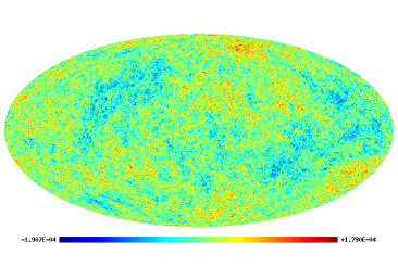
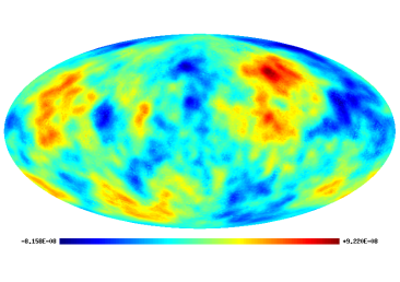
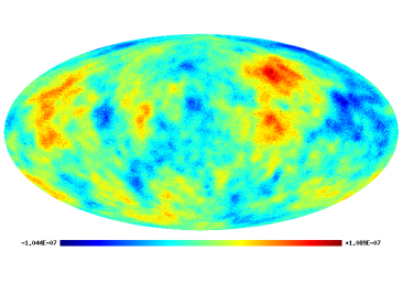
Figure 1: Represented clockwise from top left are a purely Gaussian simulation and the bispectrum simulations, computed using equation (9), for the local, equilateral and flattened models, respectively.

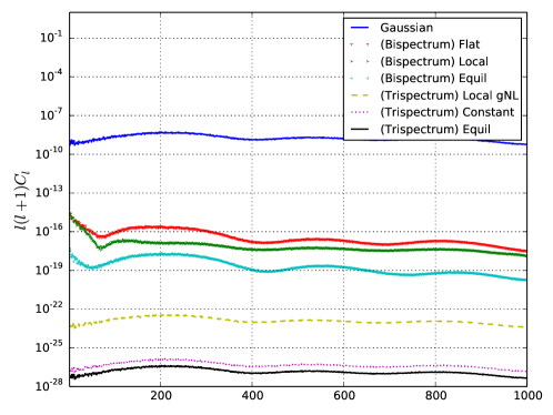
Figure 2: The power spectrum corresponding to the simulations of each of the models described in Fig. 1 is plotted. Also plotted are the power spectra computed for three (‘diagonal-free’) trispectrum models, as shall be described in §IV.4 and evaluated using equation (41). It is clear that the bispectrum and trispectrum simulations are perturbative compared to the Gaussian part at all multipoles. Plotted from top-to-bottom are the Gaussian model, the flattened, local and equilateral bispectrum models, and the local ($g_{NL}$), constant and equilateral ($c_{1}$) trispectrum models, respectively.

Needlet bispectrum estimator. We now describe the construction of an estimator for $f_{\mathrm{NL}}^{B}$ using needlets.

To define the family of needlets we will use, consider a smooth weight function $b(t)$ of compact support and satisfying the conditions

1. $b(t)>0$ only if $t\in[\mu^{-1},\mu]$ for some $\mu>1$

2. $\sum_{j=0}^{\infty}b^{2}(l/\mu^{j})=1$, for $l=1,2,\dots$ .

We pick a set of ‘scales’ $j$ which characterize the needlets used in the analysis, represents as powers of the basic scale $\mu=1.53$. For each $j$ we choose a set of $n_{\text{pix}}$ points on the sphere, labelled $k$, and denote these points $\xi_{jk}$. Then, the needlet functions $\psi_{jk}(\hat{\bm{\mathrm{{n}}}})$ are defined by

$$\psi_{jk}(\hat{\bm{\mathrm{{n}}}})=\sqrt{\lambda_{jk}}\sum_{l=\mu^{j-1}}^{\mu^{j+1}}\sum_{m=-l}^{l}b\Big{(}\frac{l}{\mu^{j}}\Big{)}Y_{lm}(\hat{\bm{\mathrm{{n}}}})Y^{*}_{lm}(\xi_{jk}),$$ (11)

where the $\lambda_{jk}$ are normalization coefficients which are proportional the the pixel area. Applied to a CMB temperature map $\Delta T(\hat{\bm{\mathrm{{n}}}})/T$ this yields needlet coefficients

$$\beta_{jk}=\int_{S^{2}}\mathrm{d}^{2}\hat{\bm{\mathrm{{n}}}}\;\frac{\Delta T(\hat{\bm{\mathrm{{n}}}})}{T}\psi_{jk}(\hat{\bm{\mathrm{{n}}}})=\sqrt{\lambda_{jk}}\sum_{l=\mu^{j-1}}^{\mu^{j+1}}\sum_{m=-l}^{l}b\left(\frac{l}{\mu^{j}}\right)a_{lm}Y_{lm}(\xi_{jk})$$ (12)

It has been shown that the mode–mode coupling introduced by masking and anisotropic noise can be accounted for by subtracting, for each scale $j$, the average over the $n_{\text{pix}}$ pixels $k$ Donzelli et al. (2012). Defining the mean for scale $j$ to be $\bar{\beta}_{j}=\sum_{k}\beta_{jk}/n_{\rm{pix}}$, this gives $\beta_{jk}\rightarrow\beta_{jk}-\bar{\beta}_{j}$. In what follows we use these subtracted quantities.

In this paper we consider the Mexican needlets defined by the weight function Scodeller et al. (2011)

$$b\left(\frac{l}{\mu^{j}}\right)=\left(\frac{l}{\mu^{j}}\right)^{2p}\exp\left(-\frac{l^{2}}{\mu^{2j}}\right),$$ (13)

and choose the coefficients $\lambda_{jk}$ to be unity. We set $p=1$, for which the Mexican needlets give a good approximation to the Spherical Mexican Hat wavelets at high frequencies, which corresponds here to large $j$.

The cubic needlet statistic is given by

$$N_{J}=\frac{1}{\sigma_{j_{1}}\sigma_{j_{2}}\sigma_{j_{3}}}\sum_{k=1}^{n_{\text{pix}}}\beta_{j_{1}k}\beta_{j_{2}k}\beta_{j_{3}k},$$ (14)

where the triplet index $J$ represents $(j_{1},j_{2},j_{3})$, and $\sigma_{j}=(4\pi)^{-1}\sum_{l}(2l+1)C_{l}b(l/\mu^{j})$. The expectation value of $N_{J}$ for a given nonlinear map can be evaluated by computing

$$\langle N_{J}^{B}\rangle=\frac{1}{\sigma_{j_{1}}\sigma_{j_{2}}\sigma_{j_{3}}}\sum_{k=1}^{n_{\text{pix}}}\langle\beta^{G}_{j_{1}k}\beta^{G}_{j_{2}k}\beta^{B}_{j_{3}k}\rangle+\text{2 perms},$$ (15)

where the superscripts ‘$G$’ and ‘$B$’ indicate needlet maps computed using, respectively, the Gaussian coefficients $a_{lm}^{G}$ and non-Gaussian coefficients $a_{lm}^{B}$ which include the bispectrum $B$. Using Eqs. (10), (12) and (15) we infer that $\langle N^{B}_{J}\rangle$ can be written

$$\langle N_{J}^{B}\rangle=\sum_{n}\bar{\alpha}_{n}^{Q}\langle N_{nJ}^{B}\rangle,$$ (16)

where the needlet maps for each mode $Q_{n}$, written $\langle N_{nJ}^{B}\rangle$, are understood to be defined by this expression. They allow for a change of basis to be performed between needlets and partial waves.

The cubic needlet statistic enables us to define an estimator for the amplitude of the bispectrum $B$ which is present in the measured CMB bispectrum. Explicitly, we have

$$\hat{f}_{\mathrm{NL}}^{B}=\frac{{\sum_{IJ}\langle N_{I}^{B}\rangle C_{IJ}^{-1}\hat{N}_{J}}}{{\sum_{IJ}\langle N_{I}^{B}\rangle C_{IJ}^{-1}\langle N_{J}^{B}\rangle}},$$ (17)

where the covariance matrix $C_{IJ}$ is defined by $C_{IJ}\equiv\langle N_{I}^{G}N_{J}^{G}\rangle-\langle N_{I}^{G}\rangle\langle N_{J}^{G}\rangle$, and

$$N_{J}^{G}=\frac{1}{\sigma_{j_{1}}\sigma_{j_{2}}\sigma_{j_{3}}n_{\text{pix}}}\sum_{k=1}^{n_{\text{pix}}}\beta^{G}_{j_{1}k}\beta^{G}_{j_{2}k}\beta^{G}_{j_{3}k}.$$ (18)

Finally, $\hat{N}_{J}$ is the cubic needlet statistic evaluated from the data. We invert the covariance matrix using principal component analysis, imposing a ratio of $10^{10}$ between the maximum and minimum eigenvalues which are retained. This approach has been used in other studies of the bispectrum using wavelets Curto et al. (2012) and needlets Donzelli et al. (2012). The 1-$\sigma$ error bar on $\hat{f}_{\mathrm{NL}}^{B}$ is

$$\sigma(\hat{f}_{\mathrm{NL}}^{B})=\Big{(}\sum_{IJ}\langle N_{I}^{B}\rangle C_{IJ}^{-1}\langle N_{J}^{B}\rangle\Big{)}^{-1/2}.$$ (19)

Using the change-of-basis matrix $\langle N_{nJ}^{B}\rangle$ we may rewrite Eq. (17) in the form

$$\hat{f}_{\mathrm{NL}}^{B}=\frac{\sum_{n}\bar{\alpha}_{n}^{Q}\langle N_{nI}^{B}\rangle C_{IJ}^{-1}N_{J}}{\sum_{nm}\bar{\alpha}_{n}^{Q}\bar{\alpha}_{m}^{Q}\sum_{IJ}\langle N_{nI}^{B}\rangle C_{IJ}^{-1}\langle N_{mJ}^{B}\rangle}=\frac{\sum_{n}\bar{\alpha}_{n}^{Q}\bar{\beta}_{n}^{Q}}{\sum_{nm}\bar{\alpha}_{n}^{Q}\gamma_{nm}\bar{\alpha}_{m}^{Q}}\,,$$ (20)

with natural definitions of $\bar{\beta}_{n}^{Q}$ and $\gamma_{nm}$ which may be deduced from this equation. Performing the Cholesky decomposition $\gamma_{nm}=\sum_{r}\lambda^{-1}_{nr}\lambda^{-1}_{mr}$, and defining $\bar{\alpha}_{r}^{R}=\sum_{n}\lambda^{-1}_{nr}\bar{\alpha}_{n}^{Q}$ and $\bar{\beta}_{r}^{R}=\sum_{n}\lambda_{rn}\bar{\beta}_{n}^{Q}$, we find that an ensemble of maps simulated with $f_{\mathrm{NL}}^{B}=1$ satisfy the consistency relation

$$\langle\bar{\beta}_{n}^{R}\rangle=\bar{\alpha}_{n}^{R}\,.$$ (21)

Thus, the coefficients $\bar{\beta}_{n}^{Q}$ recovered from the needlet maps may be used to reconstruct the underlying bispectrum shape Regan et al. (2013).

III CMB trispectrum with needlets

Primordial trispectrum. The primordial trispectrum $T_{\Phi}$ is defined by the connected four-point function of the primordial gravitational potential

$$\langle\Phi(\bm{\mathrm{{k}}}_{1})\Phi(\bm{\mathrm{{k}}}_{2})\Phi(\bm{\mathrm{{k}}}_{3})\Phi(\bm{\mathrm{{k}}}_{4})\rangle_{c}=(2\pi)^{3}\delta(\bm{\mathrm{{k}}}_{1}+\bm{\mathrm{{k}}}_{2}+\bm{\mathrm{{k}}}_{3}+\bm{\mathrm{{k}}}_{4})T_{\Phi}(\bm{\mathrm{{k}}}_{1},\bm{\mathrm{{k}}}_{2},\bm{\mathrm{{k}}}_{3},\bm{\mathrm{{k}}}_{4}).$$ (22)

In this paper we restrict attention to trispectra which are ‘diagonal’ in the sense that they can be written

$$T_{\Phi}(\bm{\mathrm{{k}}}_{1},\bm{\mathrm{{k}}}_{2},\bm{\mathrm{{k}}}_{3},\bm{\mathrm{{k}}}_{4})=p(k_{1},k_{2},k_{3},k_{4},K_{12})+p(k_{1},k_{2},k_{3},k_{4},K_{13})+p(k_{1},k_{2},k_{3},k_{4},K_{14}),$$ (23)

where $\bm{\mathrm{{K}}}_{ij}=\bm{\mathrm{{k}}}_{i}+\bm{\mathrm{{k}}}_{j}$ represents a diagonal of the quadrilateral formed by the momenta $\bm{\mathrm{{k}}}_{i}$. The zero-sum condition $\sum_{i}\bm{\mathrm{{k}}}_{i}=0$ enforced by the momentum-conservation $\delta$-function in (22) means that it is unnecessary to include the remaining combinations $\bm{\mathrm{{K}}}_{23}$, $\bm{\mathrm{{K}}}_{24}$ and $\bm{\mathrm{{K}}}_{34}$. The diagonal condition is not generic: for example, it is not satisfied by the microphysical component of the trispectrum which is generated by interactions near the epoch of horizon exit Seery et al. (2007); *Seery:2008ax; *Seery:2006js. However, Eq. (23) often does apply for phenomenological shapes generated with observable amplitude in certain models.

An interesting subclass of diagonal trispectra—including the ‘local’ $g_{\mathrm{NL}}$-shape, the $c_{1}$ equilateral trispectrum Chen et al. (2009) and the constant trispectrum Fergusson et al. (2010b)— do not depend on the diagonals $\bm{\mathrm{{K}}}_{ij}$ but only the individual side-lengths $k_{i}$. We describe these as ‘diagonal-free’. In particular, the $g_{\mathrm{NL}}$ shape satisfies

$$T_{\Phi}^{g_{\mathrm{NL}}}(k_{1},k_{2},k_{3},k_{4})=6\Big{(}P_{\Phi}(k_{1})P_{\Phi}(k_{2})P_{\Phi}(k_{3})+\text{3 perms}\Big{)}.$$ (24)

We define the shape function for diagonal-free trispectra by

$$S^{T}(k_{1},k_{2},k_{3},k_{4})=\frac{T_{\Phi}(k_{1},k_{2},k_{3},k_{4})}{T_{\Phi}^{g_{\mathrm{NL}}}(k_{1},k_{2},k_{3},k_{4})}.$$ (25)

Fergusson, Regan & Shellard Fergusson et al. (2010b) pointed out that it is possible to decompose these diagonal-free trispectra by analogy with Eq. (1). Labelling unique 4-tuples $(n_{1},n_{2},n_{3},n_{4})$ by a multi-index $n$, in the same way that we used a multi-index to label unique triplets in §II, we write

$$S^{T}(k_{1},k_{2},k_{3},k_{4})=\sum_{n}\alpha^{TQ}_{n}q^{T}_{(n_{1}}(k_{1})q^{T}_{n_{2}}(k_{2})q^{T}_{n_{3}}(k_{3})q^{T}_{n_{4})}(k_{4}).$$ (26)

The basis functions $q^{T}_{n}$ are constructed so that

$$\int_{\mathcal{V}}\Big{(}\prod_{i=1}^{4}\mathrm{d}x_{i}\Big{)}q^{T}_{n}(x_{1})q^{T}_{m}(x_{1})=\delta_{nm},$$ (27)

where the integration domain $\mathcal{V}$ is defined by the condition $\sum_{i}x_{i}>2\max\{x_{i}\}$ and $0\leqslant x_{i}\leqslant 1$. The expansion coefficients $\alpha_{n}^{TQ}$ are obtained by defining an inner product analogous to (3) and using this to construct coefficients analogous to (2). For more details on the construction of the $q_{n}^{T}$, the definition of this inner product and the calculation of the expansion coefficients $\alpha_{n}^{TQ}$ we refer to Refs. Regan et al. (2010); Fergusson et al. (2010b).

In this paper the only trispectrum we will consider which is not diagonal-free is the local $\tau_{\mathrm{NL}}$-shape given by

$$p^{\tau_{\mathrm{NL}}}(k_{1},k_{2},k_{3},k_{4};K)=\frac{25}{9}\big{(}P_{\Phi}(k_{1})+P_{\Phi}(k_{2})\big{)}\big{(}P_{\Phi}(k_{3})+P_{\Phi}(k_{4})\big{)}P_{\Phi}(K).$$ (28)

Because this cannot be decomposed using (26), we must deal with this model separately. However, as will be evident from our treatment of the trispectrum in what follows, the formalism discussed in this paper is general and applicable to arbitrary trispectra.

CMB trispectrum: diagonal-free case. The CMB trispectrum is given for diagonal-free trispectra by the connected four-point function of the spherical harmonics of the temperature map

$$\langle a_{l_{1}m_{1}}a_{l_{2}m_{2}}a_{l_{3}m_{3}}a_{l_{4}m_{4}}\rangle_{c}=t_{l_{1}l_{2}l_{3}l_{4}}\int\mathrm{d}^{2}\hat{\bm{\mathrm{{n}}}}\;Y_{l_{1}m_{1}}(\hat{\bm{\mathrm{{n}}}})Y_{l_{2}m_{2}}(\hat{\bm{\mathrm{{n}}}})Y_{l_{3}m_{3}}(\hat{\bm{\mathrm{{n}}}})Y_{l_{4}m_{4}}(\hat{\bm{\mathrm{{n}}}}).$$ (29)

where the ‘reduced’ trispectrum $t_{l_{1}l_{2}l_{3}l_{4}}$ corresponding to the diagonal-free decomposition (26) can be written Regan et al. (2010); Fergusson et al. (2010b)

$$t_{l_{1}l_{2}l_{3}l_{4}}=\sum_{n}\alpha^{TQ}_{n}\int\mathrm{d}x\,x^{2}\;\tilde{q}^{(T,2)l_{1}}_{(n_{1}}(x)\tilde{q}^{(T,-1)l_{2}}_{n_{2}}(x)\tilde{q}^{(T,-1)l_{3}}_{n_{3}}(x)\tilde{q}^{(T,-1)l_{4}}_{n_{4})}(x),$$ (30)

where $\tilde{q}^{(T,2)}_{n}$ and $\tilde{q}^{(T,-1)}_{n}$ are defined as in Eq. (5) with $q_{n}$ replaced by $q^{T}_{n}$.

We now proceed by analogy with the bispectrum, defining a transfer matrix similar to $\Gamma_{mn}$ which accounts for the line-of-sight integral over the transfer function $\Delta_{l}$, and expressing the trispectrum in terms of late-time coefficients $\bar{\alpha}^{TQ}_{n}$ analogous to those of Eq. (7). Therefore these results are limited to diagonal-free trispectra. The $\bar{\alpha}^{TQ}_{n}$, are chosen to satisfy

$$s^{T}(l_{1},l_{2},l_{3},l_{4})\equiv\frac{t_{l_{1}l_{2}l_{3}l_{4}}}{\sqrt{C_{l_{1}}C_{l_{2}}C_{l_{3}}C_{l_{4}}}}=\sum_{n}\bar{\alpha}_{n}^{T}Q_{n}^{T}(l_{1},l_{2},l_{3},l_{4}).$$ (31)

We define the inner-product $[\kern-1.5pt[f,g]\kern-1.5pt]$ by

$$[\kern-1.5pt[f,g]\kern-1.5pt]=\sum_{l_{i}}f(l_{1},l_{2},l_{3},l_{4})g(l_{1},l_{2},l_{3},l_{4})w(l_{1},l_{2},l_{3},l_{4}),$$ (32)

where the weight function $w$ satisfies

$$w_{l_{1}l_{2}l_{3}l_{4}}=\frac{1}{32\pi^{2}}\Big{[}\int_{-1}^{1}\mathrm{d}\mu\prod_{i=1}^{4}(2l_{i}+1)P_{l_{i}}(\mu)\Big{]}.$$ (33)

This choice is made so that the Fisher matrix is equal to $[\kern-1.5pt[s^{T},s^{T}]\kern-1.5pt]/24$, which will appear in Eq. (47) below. With all these choices, the late-time coefficients $\bar{\alpha}^{TQ}_{n}$ are given by

$$\bar{\alpha}_{n}^{T}=\sum_{rm}\alpha^{T}_{r}[\kern-1.5pt[\tilde{Q}_{r},Q^{T}_{m}]\kern-1.5pt]H^{-1}_{mn}=\sum_{r}\alpha^{T}_{r}\Gamma^{T}_{rn},$$ (34)

where $H_{mn}=[\kern-1.5pt[Q^{T}_{m},Q^{T}_{n}]\kern-1.5pt]$ and

$$\tilde{Q}_{n}(l_{1},l_{2},l_{3},l_{4})=(C_{l_{1}}C_{l_{2}}C_{l_{3}}C_{l_{4}})^{-1/2}\int\mathrm{d}x\;x^{2}\tilde{q}^{(T,2)l_{1}}_{(n_{1}}(x)\tilde{q}^{(T,-1)l_{2}}_{n_{2}}(x)\tilde{q}^{(T,-1)l_{3}}_{n_{3}}(x)\tilde{q}^{(T,-1)l_{4}}_{n_{4})}(x).$$ (35)

The transfer matrix for the trispectrum is defined by $\Gamma^{T}_{mn}=\sum_{r}[\kern-1.5pt[\tilde{Q}_{m},Q^{T}_{r}]\kern-1.5pt]H^{-1}_{rn}$.

CMB trispectrum: diagonal case. These results do not apply for trispectra which are not diagonal-free, such as the local $\tau_{\mathrm{NL}}$-shape (28). For a general diagonal trispectrum, the analogue of Eq. (30) is

$$\langle a_{l_{1}m_{1}}a_{l_{2}m_{2}}a_{l_{3}m_{3}}a_{l_{4}m_{4}}\rangle_{c}=\sum_{LM}(-1)^{M}\Big{[}p^{l_{1}l_{2}}_{l_{3}l_{4}}(L)\mathcal{G}^{l_{1}l_{2}L}_{m_{1}m_{2}M}\mathcal{G}^{l_{3}l_{4}L}_{m_{3}m_{4}-M}+(2\leftrightarrow 3)+(2\leftrightarrow 4)\Big{]},$$ (36)

where $\mathcal{G}^{l_{1}l_{2}L}_{m_{1}m_{2}M}\equiv\int\mathrm{d}^{2}\hat{\bm{\mathrm{{n}}}}\;Y_{l_{1}m_{1}}(\hat{\bm{\mathrm{{n}}}})Y_{l_{2}m_{2}}(\hat{\bm{\mathrm{{n}}}})Y_{LM}(\hat{\bm{\mathrm{{n}}}})$ and $(2\leftrightarrow 3)$, $(2\leftrightarrow 4)$ represent the previous expression with the labels $2$, $3$ and $2$, $4$ exchanged, respectively. For example, the local $\tau_{\mathrm{NL}}$-shape given in Eq. (28) results in the CMB trispectrum

$$p^{l_{1}l_{2}}_{l_{3}l_{4}}(L)=\int\mathrm{d}r_{1}\,\mathrm{d}r_{2}\;r_{1}^{2}r_{2}^{2}F_{L}(r_{1},r_{2})\Big{[}\alpha_{l_{1}}(r_{1})\beta_{l_{2}}(r_{1})+\alpha_{l_{2}}(r_{1})\beta_{l_{1}}(r_{1})\Big{]}\Big{[}\alpha_{l_{3}}(r_{3})\beta_{l_{4}}(r_{2})+\alpha_{l_{4}}(r_{3})\beta_{l_{3}}(r_{2})\Big{]},$$ (37)

where

$$F_{L}(r_{1},r_{2}) =\int\mathrm{d}K\;K^{2}P_{\Phi}(K)j_{L}(Kr_{1})j_{L}(Kr_{2}),$$ (38a)

$$\alpha_{l}(x) =\int\mathrm{d}k\;k^{2}\Delta_{l}(k)j_{l}(kx),$$ (38b)

$$\beta_{l}(x) =\int\mathrm{d}k\;k^{2}P_{\Phi}(k)\Delta_{l}(k)j_{l}(kx).$$ (38c)

Note that, despite the similarity of notation, $\alpha_{l}$, $\beta_{l}$ as defined here are distinct from the decomposition coefficients $\alpha_{n}^{Q}$, $\alpha_{n}^{TQ}$ and the needlet coefficients $\beta_{jk}$, $\bar{\beta}_{j}$. The definitions (38b)–(38c) are conventional.

It was shown by Pearson et al. that the following approximation is accurate to within $\lesssim 2\%$ Pearson et al. (2012),

$$p^{l_{1}l_{2}}_{l_{3}l_{4}}(L)\approx C^{\zeta_{*}}_{L}(C_{l_{1}}+C_{l_{2}})(C_{l_{3}}+C_{l_{4}}),$$ (39)

where $C^{\zeta_{*}}_{L}=(25/9)\int\mathrm{d}K\;K^{2}P_{\Phi}(K)j_{L}(Kr_{*})^{2}$ is the angular power spectrum of the curvature perturbation $\zeta$, and $r_{*}$ represents the distance to the last scattering surface.

Simulating the CMB trispectrum. As in §II we fix a choice of trispectrum $T(\bm{\mathrm{{k}}}_{1},\bm{\mathrm{{k}}}_{2},\bm{\mathrm{{k}}}_{3},\bm{\mathrm{{k}}}_{3})$ and include it in the trispectrum of the primordial gravitational potential with amplitude $g_{\mathrm{NL}}^{T}$, so that $T_{\Phi}(\bm{\mathrm{{k}}}_{1},\bm{\mathrm{{k}}}_{2},\bm{\mathrm{{k}}}_{3},\bm{\mathrm{{k}}}_{4})\supset g_{\mathrm{NL}}^{T}T(\bm{\mathrm{{k}}}_{1},\bm{\mathrm{{k}}}_{2},\bm{\mathrm{{k}}}_{3},\bm{\mathrm{{k}}}_{4})$. As for $f_{\mathrm{NL}}^{B}$, it is important to be clear that $g_{\mathrm{NL}}^{T}$ does not coincide with the traditional local $g_{\mathrm{NL}}$-parameter Okamoto and Hu (2002); *Boubekeur:2005fj; *Sasaki:2006kq unless $T$ is the conventionally-normalized local trispectrum (24). In this paper, the traditional local $g_{\mathrm{NL}}$-parameter is always denoted $g_{\mathrm{NL}}^{\text{loc}}$. Our task is to build an estimator for $g_{\mathrm{NL}}^{T}$.

To estimate the covariance matrix we must again construct averages over an ensemble of maps which contain the trispectrum $T$. For the analysis in this section, and for the constraints reported in §IV below, we will assume that there is no primordial bispectrum. It follows that we can generate appropriate maps for the temperature anisotropy by constructing multipole coefficients $a_{lm}=a_{lm}^{G}+g_{\mathrm{NL}}a_{lm}^{T}$, were $a_{lm}^{G}$ continues to be the dominant Gaussian contribution and $a_{lm}^{T}$ is a correction chosen to reproduce the trispectrum $T$. For a general trispectrum (36) we have Regan et al. (2010); Fergusson et al. (2010b)

$$a_{lm}^{T}=\frac{1}{8}\sum_{LM}\sum_{l_{i}m_{i}}(-1)^{M}p^{ll_{2}}_{l_{3}l_{4}}(L)\mathcal{G}^{ll_{2}L}_{mm_{2}M}\mathcal{G}^{l_{3}l_{4}L}_{m_{3}m_{4}-M}\frac{a_{l_{2}m_{2}}^{G*}}{C_{l_{2}}}\frac{a_{l_{3}m_{3}}^{G*}}{C_{l_{3}}}\frac{a_{l_{4}m_{4}}^{G*}}{C_{l_{4}}}\ .$$ (40)

In the case of diagonal-free trispectra we may instead use the expression Regan et al. (2010); Fergusson et al. (2010b)

$$\begin{split}a_{lm}^{T}&=\frac{1}{24}\sum_{l_{i}m_{i}}t_{ll_{2}l_{3}l_{4}}\int\mathrm{d}^{2}\hat{\bm{\mathrm{{n}}}}\;Y_{lm}(\hat{\bm{\mathrm{{n}}}})Y_{l_{2}m_{2}}(\hat{\bm{\mathrm{{n}}}})Y_{l_{3}m_{3}}(\hat{\bm{\mathrm{{n}}}})Y_{l_{4}m_{4}}(\hat{\bm{\mathrm{{n}}}})\frac{a_{l_{2}m_{2}}^{G*}}{C_{l_{2}}}\frac{a_{l_{3}m_{3}}^{G*}}{C_{l_{3}}}\frac{a_{l_{4}m_{4}}^{G*}}{C_{l_{4}}}\\ &=\frac{1}{24}\sum_{n}\alpha_{n}^{TQ}\int\mathrm{d}x\;x^{2}\int\mathrm{d}\hat{\bm{\mathrm{{n}}}}\;Y_{lm}(\hat{\bm{\mathrm{{n}}}})\Big{[}\tilde{q}^{(2)l}_{(n_{1}}(x)\tilde{M}_{n_{2}}^{(-1)(T,G)}(x,\hat{\bm{\mathrm{{n}}}})\tilde{M}_{n_{3}}^{(-1)(T,G)}(x,\hat{\bm{\mathrm{{n}}}})\tilde{M}_{n_{4})}^{(-1)(T,G)}(x,\hat{\bm{\mathrm{{n}}}})\Big{]},\end{split}$$ (41)

where $\tilde{M}_{p}^{(-1)(T,G)}(x,\hat{\bm{\mathrm{{n}}}})=\sum_{lm}\tilde{q}^{(-1,T)l}_{p}(x)a^{G}_{lm}Y_{lm}(\hat{\bm{\mathrm{{n}}}})/C_{l}$. Alternatively, using a similar approach to that described for the bispectrum, we may utilise the late-time CMB trispectrum expansion given by equation (31), and write

$$a_{lm}^{T}=\sum_{n}\bar{\alpha}_{n}^{TQ}\frac{\sqrt{C_{l}}}{24}\int\mathrm{d}\hat{\bm{\mathrm{{n}}}}\;Y_{lm}(\hat{\bm{\mathrm{{n}}}})q_{(n_{1}}\big{(}\frac{l}{l_{\text{max}}}\big{)}\bar{M}^{G}_{n_{2}}(\hat{\bm{\mathrm{{n}}}})\bar{M}^{G}_{n_{3}}(\hat{\bm{\mathrm{{n}}}})\bar{M}^{G}_{n_{4})}(\hat{\bm{\mathrm{{n}}}}),$$ (42)

where $\bar{M}^{G}_{n_{2}}(\hat{\bm{\mathrm{{n}}}})=\sum_{lm}q_{n_{2}}(l/l_{\text{max}})a_{lm}^{G}Y_{lm}(\hat{\bm{\mathrm{{n}}}})/\sqrt{C_{l}}$. Using equation (41), in Fig. 3 we plot the simulated maps for the local ($g_{\mathrm{NL}}$), equilateral ($c_{1}$) and constant trispectrum models, which will be described in §IV.4. The corresponding power spectra are plotted in Fig. 2 emphasising the perturbative nature of the trispectra compared to the Gaussian seed.

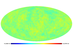
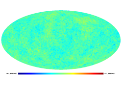
Figure 3: From left to right are the trispectrum simulations for the local ($g_{NL}$), equilateral ($c_{1}$) and constant trispectrum models, computed using equation (41).

However we choose to obtain the $a^{T}_{lm}$, we define the quartic needlet statistic by

$$N_{J}^{T}=\frac{1}{\sigma_{j_{1}}\sigma_{j_{2}}\sigma_{j_{3}}\sigma_{j_{4}}}\sum_{k=1}^{n_{\text{pix}}}\beta^{G}_{j_{1}k}\beta^{G}_{j_{2}k}\beta^{G}_{j_{3}k}\beta^{T}_{j_{4}k}+\text{3 perms},$$ (43)

where $J$ represents the unique 4-tuple $(j_{1},j_{2},j_{3},j_{4})$ and the $\beta_{jk}$ are the needlet coefficients defined in Eq. (12). A superscript ‘$G$’ indicates that these coefficients are to be computed using a Gaussian map, and the superscript ‘$T$’ indicates that they should be computed from a map which includes the trispectrum correction $a_{lm}^{T}$. We use Eq. (42) to write the expectation value of $N_{J}^{T}$ over an ensemble of maps

$$\langle N_{J}^{T}\rangle=\sum_{n}\bar{\alpha}_{n}^{TQ}\langle N_{nJ}^{T}\rangle.$$ (44)

As above, the change-of-basis matrix $\langle N_{nJ}^{T}\rangle$ is defined by this expression.

In the case of the $\tau_{\mathrm{NL}}$ trispectrum we may utilize equations (39) and (40) in order to write

$$\langle N_{J}^{T,\tau_{\mathrm{NL}}}\rangle=\sum_{L}C_{L}^{\zeta_{*}}\langle N_{LJ}^{T,\tau_{\mathrm{NL}}}\rangle\equiv\sum_{L}C_{L}^{\zeta_{*}}\sum_{M}4\int\mathrm{d}^{2}\hat{\bm{\mathrm{{n}}}}\;Y_{LM}(\hat{\bm{\mathrm{{n}}}})\tilde{\beta}_{(j_{1}}(\hat{\bm{\mathrm{{n}}}})\tilde{\beta}_{j_{2}}(\hat{\bm{\mathrm{{n}}}})\int\mathrm{d}^{2}\hat{\bm{\mathrm{{n}}}}\;Y_{LM}^{*}(\hat{\bm{\mathrm{{n}}}})\tilde{\beta}_{j_{3}}(\hat{\bm{\mathrm{{n}}}})\tilde{\beta}_{j_{4})}(\hat{\bm{\mathrm{{n}}}})\,,$$ (45)

where we express $\tilde{\beta}_{jk}$ as $\tilde{\beta}_{j}(\hat{\bm{\mathrm{{n}}}})$, with tilde representing a needlet map, (12), with appropriate weighting determined by equation (39). The beam and mask properties must also be accounted for via a transformation of these spherical harmonics, as will be described in §IV.

Needlet trispectrum estimator. In Ref. Regan et al. (2010), the Edgeworth expansion was used to derive the optimal trispectrum estimator. This was

$$\begin{split}\mathcal{E}^{\text{opt}}=&\sum_{l_{i}m_{i},l_{i}^{\prime}m_{i}^{\prime}}\big{\langle}\prod_{i=1}^{4}a_{l_{i}m_{i}}\big{\rangle}_{c}C^{-1}_{l_{1}m_{1},l_{1}^{\prime}m_{1}^{\prime}}C^{-1}_{l_{2}m_{2},l_{2}^{\prime}m_{2}^{\prime}}C^{-1}_{l_{3}m_{3},l_{3}^{\prime}m_{3}^{\prime}}C^{-1}_{l_{4}m_{4},l_{4}^{\prime}m_{4}^{\prime}}\\ &\times\Big{[}\big{(}\prod_{i=1}^{4}a_{l_{i}^{\prime}m_{i}^{\prime}}\big{)}-\big{(}C_{l_{1}^{\prime}m_{1}^{\prime},l_{2}^{\prime}m_{2}^{\prime}}a_{l_{3}^{\prime}m_{3}^{\prime}}a_{l_{4}^{\prime}m_{4}^{\prime}}+\text{5 perms}\big{)}+\big{(}C_{l_{1}^{\prime}m_{1}^{\prime},l_{2}^{\prime}m_{2}^{\prime}}C_{l_{3}^{\prime}m_{3}^{\prime},l_{4}^{\prime}m_{4}^{\prime}}+\text{2 perms}\big{)}\Big{]},\end{split}$$ (46)

where $C_{l_{1}m_{1},l_{2}m_{2}}=\langle a_{l_{1}m_{1}}a_{l_{2}m_{2}}\rangle$. Approximating the inverse covariance matrix as diagonal, i.e. $C^{-1}_{l_{1}m_{1},l_{2}m_{2}}=\delta_{l_{1},l_{2}}\delta_{m_{1},-m_{2}}(-1)^{m_{1}}C_{l_{1}}^{-1}$, it follows that the Fisher matrix $F\equiv\langle\mathcal{E}^{\rm{opt}}\rangle/24$ roughly satisfies

$$F\approx\frac{f_{\text{sky}}}{24}\sum_{l_{i}m_{i}}\frac{1}{C_{l_{1}}C_{l_{2}}C_{l_{3}}C_{l_{4}}}\big{\langle}\prod_{i=1}^{4}a_{l_{i}m_{i}}\big{\rangle}_{c}^{2},$$ (47)

where $f_{\text{sky}}$ represents the sky fraction covered by the map and $C_{l}$ is the total power spectrum, including beam effects and noise contributions. It was this approximate expression that was used in Refs. Regan et al. (2010); Fergusson et al. (2010b). A similar estimator may be derived for needlets, with the inverse covariance matrix used to optimize the signal to noise. The estimator may be used to give an estimate for the trispectrum amplitude, $\hat{g}_{\mathrm{NL}}^{T}=\mathcal{E}/\langle\mathcal{E}\rangle$. We find

$$\hat{g}_{\mathrm{NL}}^{T}=\frac{\sum_{IJ}\langle N_{I}^{T}\rangle C_{IJ}^{-1}\hat{\mathcal{N}}_{J}}{\sum_{IJ}\langle N_{I}^{T}\rangle C_{IJ}^{-1}\langle N_{J}^{T}\rangle},$$ (48)

where $\hat{\mathcal{N}}_{J}$ is to be obtained from the data,

$$\hat{\mathcal{N}}_{J}=\hat{N}_{J}-\Bigg{(}\frac{\sum_{k}\langle\beta^{G}_{j_{1}k}\beta^{G}_{j_{2}k}\rangle\hat{\beta}_{j_{3}k}\hat{\beta}_{j_{4}k}}{n_{\text{pix}}\prod_{i=1}^{4}\sigma_{j_{i}}}+\text{5 perms}\Bigg{)}+\frac{\sum_{k}\langle\beta^{G}_{j_{1}k}\beta^{G}_{j_{2}k}\beta^{G}_{j_{3}k}\beta^{G}_{j_{4}k}\rangle}{n_{\text{pix}}\prod_{i=1}^{4}\sigma_{j_{i}}},$$ (49)

with the covariance matrix defined by $C_{IJ}=\langle N_{I}^{G}N_{J}^{G}\rangle-\langle N_{I}^{G}\rangle\langle N_{J}^{G}\rangle$. The 1-$\sigma$ error bar is $\Delta\hat{g}_{\mathrm{NL}}^{T}=\langle\mathcal{E}\rangle^{-1/2}$.

For the special case of diagonal-free trispectra, where the decomposition (31) applies, we may write the trispectrum needlet map in the form (44). Then the needlet estimator becomes

$$\hat{g}_{\mathrm{NL}}=\frac{\sum_{n}\bar{\alpha}_{n}^{TQ}\langle N_{nI}^{T}\rangle C_{IJ}^{-1}\hat{\mathcal{N}}_{J}}{\sum_{nm}\bar{\alpha}_{n}^{TQ}\gamma_{nm}^{T}\bar{\alpha}_{m}^{TQ}}=\frac{\sum_{n}\bar{\alpha}_{n}^{TQ}\bar{\beta}_{n}^{TQ}}{\sum_{nm}\bar{\alpha}_{n}^{TQ}\gamma^{T}_{nm}\bar{\alpha}_{n}^{TQ}}\,,$$ (50)

where $\gamma_{nm}^{T}=\sum_{IJ}\langle N_{nI}^{T}\rangle C_{IJ}^{-1}\langle N_{mJ}^{T}\rangle$ represents the covariance matrix projected into modal space and is notationally the same as the matrix $\gamma_{nm}$ defined in Eq. (20), except that it should be computed using maps including the trispectrum contribution $T$ rather than a bispectrum contribution from $B$. In equation (50) we have defined $\bar{\beta}_{n}^{TQ}\equiv\langle N_{nI}^{T}\rangle C_{IJ}^{-1}\hat{\mathcal{N}}_{J}$.

In the case of the local $\tau_{\mathrm{NL}}$ trispectrum, using equation (45) the estimator may be written in the form

$$\hat{\tau}_{\rm{NL}}=\frac{\sum_{L}C_{L}^{\zeta_{*}}\sum_{IJ}\langle N_{LI}^{T,\tau_{\mathrm{NL}}}\rangle C_{IJ}^{-1}\mathcal{N}_{J}}{\sum_{LL^{\prime}}\sum_{IJ}C_{L}^{\zeta_{*}}\langle N_{LI}^{T,\tau_{\mathrm{NL}}}\rangle C_{IJ}^{-1}\langle N_{L^{\prime}J}^{T,\tau_{\mathrm{NL}}}\rangle C_{L^{\prime}}^{\zeta_{*}}}=\frac{\sum_{L}C_{L}^{\zeta_{*}}D_{L}}{\sum_{LL^{\prime}}C_{L}^{\zeta_{*}}G_{LL^{\prime}}C_{L^{\prime}}^{\zeta_{*}}}\,,$$ (51)

with the $1\sigma$ error bar is given by $1/\sqrt{3\sum_{LL^{\prime}}C_{L}^{\zeta_{*}}G_{LL^{\prime}}C_{L^{\prime}}^{\zeta_{*}}}$, and where the quantities $D_{L}$ and $G_{LL^{\prime}}$ may be inferred from the second and third equalities. The factor of $3$ arises due to the three instances of $p^{l_{1}l_{2}}_{l_{3}l_{4}}(L)$ in the CMB trispectrum (36). In the application of this estimator we restrict the range of $L$ to $1\leqslant L\leqslant L_{\rm{max}}=50$.

IV Application to 9-year WMAP data

In this section we apply the formalism described in §§II–III to the foreground-cleaned, coadded $V+W$ maps from the 9-year WMAP data release Bennett et al. (2013). We work up to $l_{\text{max}}=1000$. The data are supplied in HEALPix format with a resolution of $6.9$ arcmin and $N_{\text{side}}=512$, together with the necessary beam and noise properties to perform realistic simulations. In this analysis we use cosmological parameters corresponding to those of the WMAP9 fiducial cosmology, given in Table 1.

$\displaystyle\Omega_{b}h^{2}$	$\displaystyle\Omega_{c}h^{2}$	$\displaystyle\Omega_{\Lambda}$	$\displaystyle\tau$	$\displaystyle A_{\Phi}$	$\displaystyle n_{s}$
$\displaystyle 0.02256$	$\displaystyle 0.11142$	$\displaystyle 0.7185$	$\displaystyle 0.0851$	$\displaystyle 1.705\times 10^{-8}$	$\displaystyle 0.971$

Table 1: Parameters for the WMAP9 fiducial cosmology Bennett et al. (2013). The optical depth is measured by $\tau$. The parameters $A_{\Phi}$ and $n_{s}$ parametrize the primordial power spectrum, with $P_{\Phi}(k)=A_{\Phi}(k/k_{\star})^{n_{s}-1}$. The pivot scale $k_{\star}$ is chosen to be $k_{\star}=0.002h\;\text{Mpc}^{-1}$.

Simulated maps. We simulate the Gaussian spherical harmonics amplitudes $a_{lm}^{G}$ with a variance given by the angular power spectrum $C_{l}$. The non-Gaussian amplitudes $a_{lm}^{B}$ and $a_{lm}^{T}$ are simulated according to the prescriptions outlined in §§II–III, in particular Eqs. (10) and (40)–(41). We incorporate the effect of the WMAP beam $b_{l}$ and noise $n_{lm}$ for each channel $X\in\{V_{1},V_{2},W_{1},W_{2},W_{3},W_{4}\}$ by making that transformation

$$a_{lm}\rightarrow\tilde{a}_{lm}=b_{l}a_{lm}+n_{lm}.$$ (52)

For each data channel, $i$, we model $n_{lm}$ as white noise with variance per pixel given by $N_{i}(\hat{\bm{\mathrm{{n}}}})\equiv\sigma_{0,i}/\sqrt{N_{i,\text{obs}}}$ where $\sigma_{0,i}$ is the sensitivity per data channel, and $N_{i,\rm{obs}}(\hat{\bm{\mathrm{{n}}}})$ represents the corresponding number of observations per pixel. The simulations and data maps for each channel, $M_{i}(\hat{\bm{\mathrm{{n}}}})$, are coadded optimally with inverse noise weighting per pixel, i.e.

$$M(\hat{\bm{\mathrm{{n}}}})=\frac{\sum_{i\in X}M_{i}(\hat{\bm{\mathrm{{n}}}})N_{i}(\hat{\bm{\mathrm{{n}}}})^{-2}}{\sum_{i\in X}N_{i}(\hat{\bm{\mathrm{{n}}}})^{-2}},$$ (53)

where $X$ is the set of channels defined above (52).

We apply a suitable mask and remove the monopole and dipole using HEALPix. The map is then re-decomposed into spherical harmonics, and needlet maps are evaluated by convolving with the needlet function $\psi_{jk}$ as in (12). For the bispectrum we choose weight functions by setting $\mu=1.53$ and $j=0,3,4,5,\ldots,15,16$ giving fifteen distinct scales. Therefore there are ${15+2\choose 3}=680$ distinct cubic statistics $N_{J}$. For the trispectrum it is not necessary to use all scales because they provide little extra information, so we thin the range and choose $j=0,4,6,8,9,\ldots 15$. We will show later that this thinning does not impair the optimality of the estimator. These choices give $11$ distinct scales, and therefore ${11+3\choose 4}=1001$ distinct quartic statistics.

As described in §II, we subtract the mean from each wavelet coefficient, setting $\beta_{jk}\rightarrow\beta_{jk}-\bar{\beta}_{j}$, and evaluate the covariance matrix $C_{IJ}$ for the bi- and trispectrum estimators. This requires computation of the ensemble averages $\langle N_{I}N_{J}\rangle$ and $\langle N_{I}^{T}N_{J}^{T}\rangle$, together with the corresponding one-point statistics $\langle N_{I}\rangle$ and $\langle N_{I}^{T}\rangle$. For the bispectrum estimator we use a suite of $60,000$ simulations. For the trispectrum estimator we use a suite of $300,000$ simulations because we find that more samples are required to achieve convergence. The $\tau_{\mathrm{NL}}$ model requires special treatment, and it is necessary to compute its associated one-point statistic $\langle N_{I}^{\tau_{\mathrm{NL}}}\rangle$, using (45). In each case we evaluate the inverse covariance matrix $C_{IJ}^{-1}$ using principal component analysis, keeping only eigenvalues up to a factor $10^{11}$ smaller than the largest eigenvalue. We evaluate the change-of-basis matrices $\langle N_{nI}\rangle$ and $\langle N_{nI}^{T}\rangle$ using $1,000$ simulations. Finally, the trispectrum estimators (48) and (51) require the two-point expectation value $\langle\beta^{G}_{j_{1}k}\beta^{G}_{j_{2}k}\rangle$, which we obtain using $50,000$ Gaussian simulations.

At the end of this process we are able to estimate the observables $f_{\mathrm{NL}}^{B}$, $g_{\mathrm{NL}}^{T}$ and $\tau_{\mathrm{NL}}$. For $\tau_{\mathrm{NL}}$ we may immediately apply Eq. (51), whereas $f_{\mathrm{NL}}^{B}$ and $g_{\mathrm{NL}}^{T}$ first require a suitable decomposition of the primordial bi- and tri-spectra $B$ and $T$. As explained in §§II–III, for the bi- and tri-spectrum we fold the transfer function $\Delta_{l}$ and the line-of-sight integral into the respective transfer matrices $\Gamma_{nm}$ and $\Gamma^{T}_{nm}$ for computation of a decomposition of the CMB shapes.

IV.1 Validation procedure

To verify that both the cubic and quartic estimators are unbiased we apply them to $2,000$ Gaussian simulations. The mean of each recovered cubic and quartic coefficent, $\bar{\beta}_{n}^{R}$ and $\bar{\beta}_{n}^{RT}$, respectively, are verified to be consistent with zero within two standard errors of the mean. For the local bispectrum mode and local $g_{\mathrm{NL}}$-mode trispectrum we find

$$\langle\hat{f}_{\mathrm{NL}}^{\text{loc}}\rangle =0.1\pm 23.1$$ (54a)

$$\langle\hat{g}_{\mathrm{NL}}^{\text{loc}}\rangle =[0.03\pm 2.33]\times 10^{5}.$$ (54b)

The error bar for $\langle\hat{g}_{\mathrm{NL}}^{\text{loc}}\rangle$ establishes that the procedure described in this paper is close to optimal, because in Ref. Sekiguchi and Sugiyama (2013) the optimal error bar was shown to be $2.2\times 10^{5}$.

This establishes that the estimator correctly gives zero when applied to Gaussian maps, but it is also necessary to check that it recovers the correct non-Gaussian amplitude when applied to non-Gaussian maps. We test this using 200 simulations of the local-mode bispectrum and $f_{\mathrm{NL}}^{\text{loc}}=100$, constructed using the method described by Hanson et al. Hanson et al. (2009). We recover the result $\langle\hat{f}_{\mathrm{NL}}^{\text{loc}}\rangle=100.3\pm 0.34$, where the error bar represents the standard error of the mean.

In Fig. 4 we plot the eigenvalues for both the bispectrum (cubic statistics) and trispectrum (quartic statistics), in order to assess the number of elements included in the analysis after applying principal-component analysis to the covariance matrix. The indicated cutoff value is $10^{-11}$ times the maximum eigenvalue.

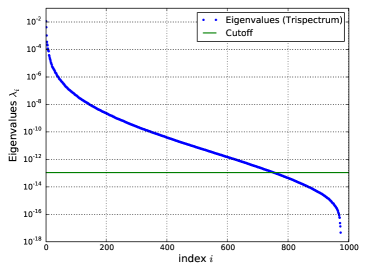
Figure 4: Plotted are the principal eigenvalues of the covariance matrix for the cubic (left) and quartic (right) needlet statistics. The cutoff value of $10^{-11}$ times the maximum eigenvalue applied in the inversion of the covariance matrix is also indicated in both cases.

IV.2 Point source Simulations

To estimate the effect of unresolved point sources we adopt the constant-flux model described in Ref. Komatsu et al. (2009). We assume that a population of sources, each with constant flux $F_{\text{src}}$, and number density $n_{\text{src}}$ per steradian, contaminate each pixel with a frequency-dependent temperature increment $\delta T_{\text{src}}(\hat{\bm{\mathrm{{n}}}})=F_{\text{src}}g(x)\epsilon(\hat{\bm{\mathrm{{n}}}})/\Omega_{\text{pix}}$, where $\Omega_{\text{pix}}=1/n_{\text{pix}}$ is the solid angle per pixel and $x=h\nu/k_{\text{B}}T_{\text{CMB}}=\nu/(56.8\,\text{GHz})$. The function $g(x)$ satisfies

$$g(x)=\frac{\sinh^{2}(x/2)}{x^{4}}\frac{1}{24.8\;\text{Jy}\,\text{K}^{-1}\,\text{sr}^{-1}}$$ (55)

and represents the conversion factor between brightness and temperature Tegmark and Efstathiou (1996). Finally, $\epsilon(\hat{\bm{\mathrm{{n}}}})$ is a Poisson-distributed random variable with mean $n_{\text{src}}\Omega_{\text{pix}}$. This Poisson distribution of sources introduces a non-Gaussian signature. This constant-flux model satisfactorily reproduces the power spectrum and bispectrum of point sources measured by the WMAP team Komatsu et al. (2009); Nolta et al. (2009), given the values $F_{\text{src}}=0.5\;\text{Jy}$ and a source density of $n_{\text{src}}=85\;\text{sr}^{-1}$.

To estimate the influence of point sources on the estimators described above, we perform a separate set of $1,000$ simulations in which we construct a set of Gaussian maps using (52) and (53). These maps are modified by adding a point-source contamination according to the prescription above. We compute the cubic and quartic needlet statistics both with and without point sources. Taking the difference for each realization gives an estimate of the bias on $f_{\mathrm{NL}}^{B}$ or $g_{\mathrm{NL}}^{T}$ for each primordial shape of interest. We give numerical results in Table 2.

IV.3 Bispectrum Constraints

In this section we tabulate the constraints and estimated point source contamination for the local, DBI, equilateral, constant, orthogonal and flattened bispectrum models. Constraints for these models have previously been published by Fergusson, Liguori & Shellard based on the KSW estimator Fergusson et al. (2012) and using a wavelet-based estimator in Ref. Regan et al. (2013).

• Local model. A Taylor expansion around a Gaussian gravitational potential $\phi_{G}$ defines both the local-mode bispectrum and local $g_{\mathrm{NL}}$-mode trispectrum. It accurately represents the type of non-Gaussianity generated by evolution on superhorizon scales in multiple-field inflationary models Lyth and Rodriguez (2005); Seery and Lidsey (2007) or the curvaton model Enqvist and Sloth (2002); Lyth and Wands (2002); Moroi and Takahashi (2001). We write Salopek and Bond (1990)

  $$\Phi(\bm{\mathrm{{x}}})=\Phi_{G}(\bm{\mathrm{{x}}})+f_{\mathrm{NL}}^{\text{loc}}(\Phi_{G}(\bm{\mathrm{{x}}})^{2}-\langle\Phi_{G}(\bm{\mathrm{{x}}})^{2}\rangle)+g_{\mathrm{NL}}^{\text{loc}}\Phi_{G}(\bm{\mathrm{{x}}})^{3}+\dots\,.$$ (56)

  The resulting primordial bispectrum is given by

  $$B_{\Phi}(k_{1},k_{2},k_{3})=2f_{\mathrm{NL}}^{\text{loc}}(P_{\Phi}(k_{1})P_{\Phi}(k_{2})+P_{\Phi}(k_{1})P_{\Phi}(k_{3})+P_{\Phi}(k_{2})P_{\Phi}(k_{3})).$$ (57)

  Our constraints on $f_{\mathrm{NL}}^{\text{loc}}$ and the bias $\Delta f_{\mathrm{NL}}^{\text{loc}}$ due to point sources are

  $$f_{\mathrm{NL}}^{\text{loc}}=38.6\pm 23.1\quad\text{and}\quad\Delta f_{\mathrm{NL}}^{\text{loc}}=9.6\pm 4.1.$$ (58)

  This result is consistent with the needlet-based constraint $f_{\mathrm{NL}}^{\text{loc}}=37.5\pm 21.8$ reported by Donzelli et al. Donzelli et al. (2012), and with the wavelet-based constraint $f_{\mathrm{NL}}^{\text{loc}}=38.4\pm 23.6$ reported in Ref. Regan et al. (2013).

  The lower error bar in the case of Donzelli et al. Donzelli et al. (2012) may be partly attributed to the larger number of needlet scales used in that work, as well as the use of a linear term correction. We have chosen to ignore the linear correction term in this work, because Refs. Curto et al. (2012); Regan et al. (2013) demonstrated (in the case of wavelets) that it leads to only a $\lesssim 2\%$ correction; the mean scale subtraction largely accounting for anisotropies due to the mask and noise. In addition the remaining bispectrum models achieve optimality and therefore we persist with only $15$ needlet scales. However, we note that to achieve optimality in the case of the local model, we may require more scales. While this issue is somewhat parenthetic to the aims of this paper, we present an investigation of the dependency of the results on the maximum and minimum needlet scale in Fig. 5.

  The estimate for the bias due to point sources given in (58) for the contribution of point sources is larger than predicted using wavelets, which give $\Delta f_{\mathrm{NL}}^{\text{loc}}=3.1\pm 3.7$ Regan et al. (2013).

• DBI and equilateral models. Under certain circumstances, non-standard kinetic terms may lead to strong self-interactions between modes as they leave the horizon Alishahiha et al. (2004); Chen et al. (2007a, b). An example is DBI inflation, for which the equilateral model provides an accurate separable approximation. The bispectra are

  $$B_{\Phi}^{\text{DBI}} =\frac{1}{(k_{1}k_{2}k_{3})^{3}(\sum_{i}k_{i})^{2}}\bigg{(}\sum_{i}k_{i}^{5}+\sum_{i\neq j}(2k_{i}^{4}k_{j}-3k_{i}^{3}k_{j}^{2})+\sum_{i\neq j\neq l}(k_{i}^{3}k_{j}k_{l}-4k_{i}^{2}k_{j}^{2}k_{l})\bigg{)},$$ (59)

  $$B_{\Phi}^{\text{eq}} =6\bigg{(}-\Big{[}P_{\Phi}(k_{1})P_{\Phi}(k_{2})+\text{2 perms}\Big{]}-2\Big{[}P_{\Phi}(k_{1})P_{\Phi}(k_{2})P_{\Phi}(k_{3})\Big{]}^{2/3}+\Big{[}P_{\Phi}^{1/3}(k_{1})P_{\Phi}^{2/3}(k_{2})P_{\Phi}(k_{3})+\text{5 perms}\Big{]}\bigg{)}.$$ (60)

  The needlet-based estimator gives

  $$f_{\mathrm{NL}}^{\text{DBI}} =65.5\pm 99.4 \Delta f_{\mathrm{NL}}^{\text{DBI}} =9.5\pm 14.1\,,$$

  $$f_{\mathrm{NL}}^{\text{eq}} =64.5\pm 117.3 \Delta f_{\mathrm{NL}}^{\text{eq}} =11.0\pm 19.3\,.$$ (61)

• Constant model. The constant model gives a primordial bispectrum corresponding to

  $$B^{\text{const}}_{\Phi}(k_{1},k_{2},k_{3})=6(P_{\Phi}(k_{1})P_{\Phi}(k_{2})P_{\Phi}(k_{3}))^{2/3}.$$ (62)

  The CMB bispectrum is entirely due to the transfer function; see Ref. Chen and Wang (2010) for a possible microphysical realization. The needlet estimator gives

  $$f_{\mathrm{NL}}^{\text{const}}=60.8\pm 62.7\quad\qquad\Delta f_{\mathrm{NL}}^{\text{const}}=9.3\pm 9.9.$$ (63)

• Orthogonal model. The orthogonal model is given by a linear combination of the equilateral and constant models, $B^{\rm{orthog}}_{\Phi}=3B^{\rm{eq}}_{\Phi}-2B^{\rm{const}}_{\Phi}$. We obtain

  $$f_{\mathrm{NL}}^{\text{orthog}}=-175.0\pm 101.8\quad\qquad\Delta f_{\mathrm{NL}}^{\text{orthog}}=-24.3\pm 16.7.$$ (64)

  For comparison, the constraint from 7-year WMAP data using the wavelet-based estimator of Ref. Regan et al. (2013) was $f_{\mathrm{NL}}^{\text{orthog}}=-173.2\pm 101.4$. By comparison, the WMAP team report $f_{\mathrm{NL}}^{\text{orthog}}=-245\pm 100$ from the 9-year data Bennett et al. (2013). The constraint given in (64) uses 9-year data and is consistent with the 7-year result. It is substantially less significant than the result obtained by the WMAP team. Below, we investigate this further by providing a frequency-band analysis.

• Flattened model. A ‘flattened’ configuration may be produced by a nontrivial initial state, including a non-Bunch–Davies vacuum. For such states, long-lived excitations with nearly zero energy can be formed by a combination of positive- and negative-energy modes. These generate strong correlations. Physical models realizing this effect are discussed, for example, in Refs. Holman and Tolley (2008); Ashoorioon and Shiu (2011). The bispectrum is

  $$B_{\Phi}^{\text{flat}}=\frac{6}{39(k_{1}k_{2}k_{3})^{2}}\Bigg{[}\left(\frac{k_{1}^{2}+k_{2}^{2}-k_{3}^{2}}{k_{2}k_{3}}+\text{2 perms}\right)+12+8\left(\frac{k_{1}k_{2}+k_{1}k_{3}-k_{2}k_{3}}{(k_{2}+k_{3}-k_{1})^{2}}+\text{2 perms}\right)\Bigg{]}\,.$$ (65)

  In order to handle the divergence we set the bispectrum to zero for $k_{1}+k_{2}-k_{3}<Z\sum_{i}k_{i}$ (or its permutations) with $Z=0.03$ and employ a low pass (Gaussian) filter in order to smoothen the shape near the edges as in Ref. Fergusson et al. (2010a). The resulting constraints are

  $$f_{\mathrm{NL}}^{\text{flat}}=14.9\pm 10.5\qquad\Delta f_{\mathrm{NL}}^{\text{flat}}=2.5\pm 1.7.$$ (66)

				Point source contamination
Shape	V-band	W-band	V+W	V-band	W-band	V+W
Local	$\displaystyle 44.0\pm 26.2$	$\displaystyle 30.2\pm 26.6$	$\displaystyle 38.6\pm 23.1$	$\displaystyle 12.0\pm 5.1$	$\displaystyle 1.6\pm 2.4$	$\displaystyle\,\,\,9.6\pm 4.1$
DBI	$\displaystyle 53.3\pm 106.4$	$\displaystyle 86.4\pm 107.2$	$\displaystyle 65.5\pm 99.4$	$\displaystyle 31.9\pm 18.5$	$\displaystyle 3.5\pm 9.1$	$\displaystyle\,\,\,9.5\pm 16.1$
Equilateral	$\displaystyle 54.2\pm 125.6$	$\displaystyle 88.6\pm 126.7$	$\displaystyle 64.5\pm 117.3$	$\displaystyle 38.3\pm 22.2$	$\displaystyle 4.4\pm 10.9$	$\displaystyle\,\,\,11.0\pm 19.3$
Constant	$\displaystyle 54.1\pm 67.5$	$\displaystyle 85.1\pm 67.6$	$\displaystyle 60.8\pm 62.7$	$\displaystyle 22.8\pm 11.6$	$\displaystyle 2.6\pm 5.7$	$\displaystyle\,\,\,9.3\pm 9.9$
Orthogonal	$\displaystyle-154.7\pm 114.9$	$\displaystyle-182.8\pm 114.0$	$\displaystyle-175.0\pm 101.8$	$\displaystyle-36.0\pm 20.1$	$\displaystyle-3.9\pm 9.6$	$\displaystyle\,\,\,-24.3\pm 16.7$
Flat	$\displaystyle 13.1\pm 11.6$	$\displaystyle 15.6\pm 11.6$	$\displaystyle 14.9\pm 10.5$	$\displaystyle 4.7\pm 2.1$	$\displaystyle 0.6\pm 1.0$	$\displaystyle\,\,\,2.5\pm 1.7$

Table 2: Constraints on the various bispectrum shapes computed for, respectively, the V-band, W-band and coadded data. The last three columns give estimates for the point source contamination in each case.

Frequency dependence. Instead of using the entire dataset, it is possible to obtain constraints using only V- or W-band data and corresponding simulations of the maps and covariance matrix. The bias due to point sources can be taken into account as described above. We tabulate our results in Tables 2 and 3.

We find that point-source contamination in the V-band is more significant than in the W-band. In comparison to alternative estimators, such as Spherical Mexican Hat wavelets, needlets show more sensitivity to point-source contamination of the local shape. The frequency-band analysis shows that the V- and W-band constraints are consistent for each model (within 1-$\sigma$), including for the orthogonal shape for which the WMAP team obtained discrepant results from the 9-year data Bennett et al. (2013) ($f_{\mathrm{NL}}^{\text{orthog}}=-245.5\pm 99.6$ from the coadded map, $f_{\mathrm{NL}}^{\text{orthog}}=-125.9\pm 112.7$ from V-band only, and $f_{\mathrm{NL}}^{\text{orthog}}=-320.2\pm 112.1$ from W-band only). The needlet-based analysis given here produces much weaker frequency dependence.

Shape	V-band	W-band	V+W
Local	$\displaystyle 32.0\pm 26.2$	$\displaystyle 28.6\pm 26.6$	$\displaystyle 29.0\pm 23.1$
DBI	$\displaystyle 21.4\pm 106.4$	$\displaystyle 82.9\pm 107.2$	$\displaystyle 56.0\pm 99.4$
Equilateral	$\displaystyle 15.9\pm 125.6$	$\displaystyle 84.2\pm 126.7$	$\displaystyle 53.5\pm 117.3$
Constant	$\displaystyle 31.3\pm 67.5$	$\displaystyle 82.5\pm 67.6$	$\displaystyle 51.5\pm 62.7$
Orthogonal	$\displaystyle-118.7\pm 114.9$	$\displaystyle-178.9\pm 114.0$	$\displaystyle-150.7\pm 101.8$
Flat	$\displaystyle 8.4\pm 11.6$	$\displaystyle 15.0\pm 11.6$	$\displaystyle 12.4\pm 10.5$

Table 3: Constraints on bispectrum models corrected for the effect of point sources (see Table 2).

Point Source Model Investigation. One may be concerned that the constant-flux point source model described in §IV.2 is too simplistic. Therefore, we also implement a more realistic point source model which provides a better match to observations at each flux value. We use the analytic fit Argueso et al. (2006) to the de Zotti et al. De Zotti et al. (2005) observations, with the proper distribution of number counts $dn/dS=AS^{-\alpha}$, where $A=22.1\pm 1.5$ and $\alpha=2.32\pm 0.06$ with the best fit value chosen for our simulations. Extending the constant-flux model we integrate over fluxes using this model with $S\in[10^{-3},1]\,{\rm Jy}$. In Table 4 we list the corresponding estimates for the contamination due to point sources. Comparison to Table 2 reveals the consistency of the results obtained using both point source models. In the context of searches for primordial non-Gaussianity beyond Planck, more detailed source modelling may be necessary. Indeed, the extra intensity of the point source contamination in the V-band suggests the impact of radio-sources. A study of different families of point sources was performed in Ref. Curto et al. (2013) detailing the potentially strong non-Gaussian deviations due to unresolved point sources for both high $(>225{\rm GHz})$ and low $(<100{\rm GHz})$ frequency data.

Shape	V-band	W-band	V+W
Local	$\displaystyle 15.3\pm 5.3$	$\displaystyle 2.2\pm 7.1$	$\displaystyle 10.8\pm 4.8$
DBI	$\displaystyle 37.4\pm 23.7$	$\displaystyle 6.6\pm 13.7$	$\displaystyle 7.5\pm 11.1$
Equilateral	$\displaystyle 44.4\pm 27.2$	$\displaystyle 8.0\pm 15.6$	$\displaystyle 7.9\pm 17.0$
Constant	$\displaystyle 27.4\pm 13.2$	$\displaystyle 4.6\pm 10.1$	$\displaystyle 8.9\pm 8.9$
Orthogonal	$\displaystyle-47.3\pm 23.3$	$\displaystyle-6.8\pm 22.6$	$\displaystyle-29.2\pm 18.6$
Flat	$\displaystyle 5.8\pm 1.9$	$\displaystyle 0.9\pm 2.1$	$\displaystyle 2.7\pm 1.6$

Table 4: Estimates for the point source contamination for each bispectrum model considered, for the V-, W- and coadded data, using the more realistic point source model. Comparison to Table 2 reveals the consistency with the results obtained using the more simplistic constant flux model.

Needlet scale dependence. In order to assess the dependence of our results on the needlet scales, in Fig. 5 we present (in the left hand column) a plot of the best-fit value and the error bar of $f_{\mathrm{NL}}$, as we include more needlet scales, up to the maximum scale used in our analysis. On the right hand column we plot the corresponding quantities as we increase the minimum needlet scale. For each case it is necessary to recompute the inverse covariance matrix for the needlet scales under consideration. We present the plots for the local, equilateral and flattened models, noting that the other models considered in this work may be represented as linear combinations of these. The equilateral and flattened models are largely insensitive to the maximum and minimum scale chosen, supporting the observation that we have achieved optimal error bars for each. In the case of the local model there is the possibility that the error bars may shrink slightly with an increased number of needlet scales, as detailed earlier in the section. Nevertheless, the results show the robustness of our results to the choice of scales used.

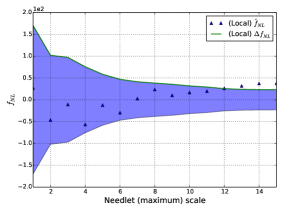
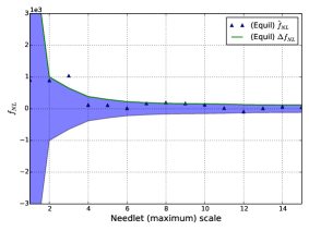
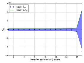
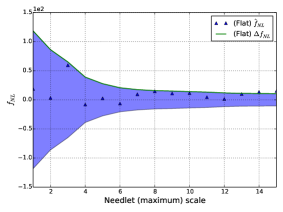
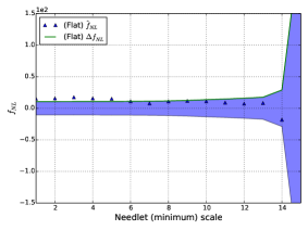
Figure 5: Plotted on the left column is the dependency of the best fit value - and error bar - of $f_{\mathrm{NL}}$ on the maximum needlet scale. The triangle glyph represents the best fit value, while shading is used to represent the region $f_{\mathrm{NL}}\in[-\Delta f_{\mathrm{NL}},\Delta f_{\mathrm{NL}}]$. Represented are the constraints using all measured needlet data up to the maximum scale indicated. On the right hand column we represent the dependency on the minimum needlet scale, with all needlet data used beyond this scale. From top to bottom we plot these quantities for the local, equilateral and flattened models respectively.

IV.4 Trispectrum Constraints

By comparison with the bispectrum, obtaining constraints on the CMB trispectrum is numerically challenging. Here we briefly review constraints which have appeared in the literature. Desjacques and Seljak found the constraint $\hat{g}_{\mathrm{NL}}^{\text{loc}}=[2.35\pm 2.93]\times 10^{5}$ using the scale-dependent bias of dark matter haloes in the local model Desjacques and Seljak (2010). Smidt et al. used a pseudo-$C_{l}$ estimator to obtain $\hat{g}_{\mathrm{NL}}^{\text{loc}}=[0.4\pm 3.9]\times 10^{5}$ Smidt et al. (2010). Using a modal decomposition and a suboptimal trispectrum estimator, working up to $l_{\text{max}}=500$, Regan et al. found $\hat{g}_{\mathrm{NL}}^{\text{loc}}=[1.1\pm 4.9]\times 10^{5}$ Regan et al. (2010); Fergusson et al. (2010b). Recently, Sekiguchi & Sugiyama, using $l_{\text{max}}=1024$, established that the optimal error bar for the local $g_{\mathrm{NL}}$-mode is $2.2\times 10^{5}$, finding $\hat{g}_{\mathrm{NL}}^{\text{loc}}=[-3.3\pm 2.2]\times 10^{5}$. Their analysis implemented the optimal estimator developed in Ref. Regan et al. (2010), using the full pixel-by-pixel inverse covariance matrix. In this paper we work up to $l_{\text{max}}=1000$, with the pixel-based estimator replaced by a needlet estimator. This has the advantage that, instead of inverting an $\sim 10^{6}\times 10^{6}$ matrix representing the pixel-by-pixel covariance, we need only invert a $\sim 10^{3}\times 10^{3}$ matrix representing the covariance between needlets. Nevertheless, this only results in a small loss of optimality.

• Local $g_{\mathrm{NL}}$ model. The local model was discussed in §IV.3. It gives a trispectrum of the form (24). We find

  $$g_{\mathrm{NL}}^{\text{loc}}=[-2.3\pm 2.3]\times 10^{5}\quad\text{and}\quad\Delta g_{\mathrm{NL}}^{\text{loc}}=[1.8\pm 2.2]\times 10^{5}$$ (67)

  where (estimated here for the first time) $\Delta g_{\mathrm{NL}}^{\text{loc}}$ represents the bias due to point sources. Correcting for this bias, the constraint $g_{\mathrm{NL}}^{\text{loca}}=[-4.1\pm 2.3]\times 10^{5}$ is within $\lesssim 5\%$ of the optimal bound and is consistent with the result reported by Sekiguchi & Sugiyama Sekiguchi and Sugiyama (2013). This represents strong evidence in favour of the accuracy and efficacy of the needlet-based estimator.

  The point source constraints reported are calculated using the more accurate model described in the previous section. Using the simpler constant flux model, the point source constraint is calculated to be $\Delta g_{\mathrm{NL}}^{\text{loc}}=[0.9\pm 2.2]\times 10^{5}$. Thus it appears that the constant flux model underestimates the bias due to point sources. However, as we shall see this simple model works well for the other trispectrum models considered, and we will not pursue this interesting issue further in this paper. It is worth noting, however, that the trispectrum constraints appear to show stronger dependency on the presence of point sources than those of the bispectrum. We also consider the dependency of the results on the maximum needlet scale considered. In Fig. 6 the best-fit and $1\sigma$ error bars are plotted as a function of the maximum needlet scale chosen, up until the maximum used in our data analysis. The results show the convergence to the reported values, indicating the robustness of the reported values on the needlet scales chosen.

  

  

  

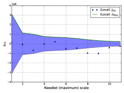
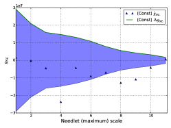
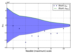
  Figure 6: Represented left to right are the dependencies of best-fit (triangular glyphs) and $1\sigma$error bars on the maximum needlet scale used for the local $g_{NL}$ model, the constant trispectrum, and the equilateral, $c_{1}$, trispectrum, respectively.

• Constant model. The constant trispectrum was defined in Ref. Fergusson et al. (2010b) by analogy with the constant bispectrum. It gives

  $$T_{\Phi}(k_{1},k_{2},k_{3},k_{4})=24\big{(}P_{\Phi}(k_{1})P_{\Phi}(k_{2})P_{\Phi}(k_{3})P_{\Phi}(k_{4})\big{)}^{3/4}.$$ (68)

  As with the constant bispectrum, features in this model are entirely due to the transfer functions. We find

  $$g_{\mathrm{NL}}^{\text{const}}=[0.8\pm 1.8]\times 10^{6}\quad\text{and}\quad\Delta g_{\mathrm{NL}}^{\text{const}}=[1.0\pm 1.6]\times 10^{6}.$$ (69)

  Correcting for the bias due to point sources this is equivalent to $g_{\mathrm{NL}}^{\text{const}}=[-0.2\pm 1.8]\times 10^{6}$ and improves on the (corrected) constraint $g_{\mathrm{NL}}^{\text{const}}=[1.0\pm 2.8]\times 10^{6}$ presented in Ref. Fergusson et al. (2010b). The point source constraint uses the more accurate point source model but is very consistent with the constant flux model which gives $\Delta g_{\mathrm{NL}}^{\text{const}}=[0.8\pm 1.6]\times 10^{6}$. In Fig. 6 we plot the dependency of the results on the (maximum) needlet scale used in the analysis. There appears to be a weak dependency on the maximum scale chosen, but the results clearly support the robust conclusion that the best-fit value lies within $\sim 1\sigma$ of zero.

• Equilateral $c_{1}$ model. In Refs. Chen et al. (2009, 2006); Arroja et al. (2009) it was demonstrated that the trispectrum for single-field inflation models with nontrivial kinetic terms receives its dominant contribution from a combination of three trispectra $T_{s_{1},s_{2},s_{3}}$ generated by scalar exchange, and three trispectra $T_{c_{1},c_{2},c_{3}}$ generated by contact interactions. As explained in Ref. Fergusson et al. (2010b), the $c_{1}$-type contact-interaction trispectrum is strongly correlated with most of the other shapes. Helpfully, it can be described by a simple diagonal-free formula, for which

  $$T_{c_{1}}(k_{1},k_{2},k_{3},k_{4})=\frac{24A_{\Phi}^{3}}{k_{1}k_{2}k_{3}k_{4}(\sum_{i}k_{i}/4)^{5}}.$$ (70)

  We find the constraints

  $$g_{\mathrm{NL}}^{c_{1}}=[0.8\pm 2.9]\times 10^{6}\quad\text{and}\quad\Delta g_{\mathrm{NL}}^{c_{1}}=[1.6\pm 2.5]\times 10^{6}.$$ (71)

  The constraint after correction for biasing is $g_{\mathrm{NL}}^{c_{1}}=[-0.8\pm 2.9]\times 10^{6}$. This is again consistent with the (corrected) result of Ref. Fergusson et al. (2010b), which found $g_{\mathrm{NL}}^{c_{1}}=[-2.4\pm 5.8]\times 10^{6}$. As for the constant model, the constraint on the point sources is largely insensitive to the model used with the constant flux model giving the constraint $\Delta g_{\mathrm{NL}}^{c_{1}}=[1.2\pm 2.5]\times 10^{6}$. In addition, the plot of the dependency on the maximum needlet scale in Fig. 6 further supports the conclusion that the best-fit value lies within $\sim 1\sigma$ of zero.

• Local $\tau_{\mathrm{NL}}$ model. The local model (56) also generates a trispectrum in the $\tau_{\mathrm{NL}}$-mode, which gives $\tau_{\mathrm{NL}}^{\text{loc}}=(6f_{\mathrm{NL}}^{\text{loc}}/5)^{2}$. In models with more contributions to the curvature perturabtion this is softened to an inequality $\tau_{\mathrm{NL}}^{\text{loc}}\geqslant(6f_{\mathrm{NL}}^{\text{loc}}/5)^{2}$ Suyama and Yamaguchi (2008); Smith et al. (2011); Assassi et al. (2012). Therefore, simultaneous detections of $\tau_{\mathrm{NL}}^{\text{loc}}$ and $f_{\mathrm{NL}}^{\text{loc}}$ would provide an opportunity to probe the microphysics of the inflationary era.

  Unfortunately, estimating $\tau_{\mathrm{NL}}^{\text{loc}}$ is a challenging undertaking. Ref. Regan et al. (2010) derived the estimator $\hat{\tau}_{\mathrm{NL}}^{\text{loc}}=\mathcal{E}^{\tau_{\mathrm{NL}}}/\langle\mathcal{E}^{\tau_{\mathrm{NL}}}\rangle$, where

  $$\begin{split}\mathcal{E}^{\tau_{\mathrm{NL}}}=3&\sum_{l_{i}m_{i}}\sum_{LM}(-1)^{M}p^{l_{1}l_{2}}_{l_{3}l_{4}}(L)\mathcal{G}^{l_{1}l_{2}L}_{m_{1}m_{2}M}\mathcal{G}^{l_{3}l_{4}L}_{m_{3}m_{4}-M}\\ &\mbox{}\times\Bigg{(}\prod_{i=1}^{4}\tilde{a}_{l_{i}m_{i}}-\Big{(}\langle\tilde{a}^{G}_{l_{1}m_{1}}\tilde{a}^{G}_{l_{2}m_{2}}\rangle\tilde{a}_{l_{3}m_{3}}\tilde{a}_{l_{4}m_{4}}+\text{5 perms}\Big{)}+\langle\tilde{a}^{G}_{l_{1}m_{1}}\tilde{a}^{G}_{l_{2}m_{2}}\rangle\langle\tilde{a}^{G}_{l_{3}m_{3}}\tilde{a}^{G}_{l_{4}m_{4}}\rangle+\text{2 perms})\Bigg{)}\end{split}$$ (72)

  $$\begin{split}\langle\mathcal{E}^{\tau_{\mathrm{NL}}}\rangle\approx 3\sum_{l_{i},L}\frac{p^{l_{1}l_{2}}_{l_{3}l_{4}}(L)h_{l_{1}l_{2}L}h_{l_{3}l_{4}L}}{C_{l_{1}}C_{l_{2}}C_{l_{3}}C_{l_{4}}}\Bigg{(}&\frac{p^{l_{1}l_{2}}_{l_{3}l_{4}}(L)h_{l_{1}l_{2}L}h_{l_{3}l_{4}L}}{2L+1}+\sum_{L^{\prime}}(-1)^{l_{2}+l_{3}}\Big{\{}\begin{array}[]{ccc}l_{1}&l_{2}&L\\ l_{4}&l_{3}&L^{\prime}\end{array}\Big{\}}p^{l_{1}l_{3}}_{l_{2}l_{4}}(L^{\prime})h_{l_{1}l_{3}L^{\prime}}h_{l_{2}l_{4}L^{\prime}}\\ &\mbox{}+\sum_{L^{\prime}}(-1)^{L+L^{\prime}}\Big{\{}\begin{array}[]{ccc}l_{1}&l_{2}&L\\ l_{3}&l_{4}&L^{\prime}\end{array}\Big{\}}p^{l_{1}l_{4}}_{l_{3}l_{2}}(L^{\prime})h_{l_{1}l_{4}L^{\prime}}h_{l_{3}l_{2}L^{\prime}}\Bigg{)},\end{split}$$ (73)

  where $\tilde{a}_{lm}=(C^{-1}a)_{lm}$ are the inverse-covariance weighted spherical harmonics and

  $$h_{l_{1}l_{2}l_{3}}\equiv\sqrt{\frac{\prod_{i=1}^{3}(2l_{i}+1)}{4\pi}}\Big{(}\begin{array}[]{ccc}l_{1}&l_{2}&l_{3}\\ 0&0&0\end{array}\Big{)}.$$ (74)

  We have expressed $\langle\mathcal{E}^{\tau_{\mathrm{NL}}}\rangle$ using the approximation of a diagonal covariance matrix. Unfortunately, the presence of the $6j$ symbols $\{\dots\}$ means that the computation of $\langle\mathcal{E}^{\tau_{\mathrm{NL}}}\rangle$ is prohibitive and therefore some approximations are required. For example, it is an accurate approximation to restrict the calculation to $L\lesssim 100$ and neglect the effect of the $6j$ symbols Kogo and Komatsu (2006).

  However, the needlet estimator (51) obviates this by removing the necessity to calculate the $6j$ symbols explicitly. Nevertheless, the $\tau_{\mathrm{NL}}$ model still represents a formidable numerical challenge due to the presence of two line-of-sight integrals in (37).

  To make progress, we use the observation of Pearson et al. Pearson et al. (2012) that Eq. (39) represents an accurate approximation to the $\tau_{\mathrm{NL}}$ trispectrum shape. In this paper we employ it for the calculation of expectation values of the quartic needlet statistic, Eq. (45). We note that a similar approximation could be applied to the trispectrum generated by cosmic strings, or due to lensing.

  Alternative approaches are possible. A modulation-based estimator was developed by Pearson et al. Pearson et al. (2012) and was applied to Planck data for the Planck2013 data release Planck Collaboration et al. (2013). This modulation-based estimator is similar to Eq. (72) with (39) used to approximate the $\tau_{\mathrm{NL}}$-mode trispectrum. That is,

  $$\mathcal{E}^{\tau_{\mathrm{NL}}}_{\text{mod}}=12\sum_{L}C_{L}^{\zeta_{*}}\sum_{M}\Big{(}|f_{LM}-\langle f_{LM}\rangle|^{2}-\langle|f_{LM}^{G}-\langle f_{LM}^{G}\rangle|^{2}\rangle\Big{)},$$ (75)

  where

  $$f_{LM}=\int\mathrm{d}^{2}\hat{\bm{\mathrm{{n}}}}\;Y_{LM}^{*}(\hat{\bm{\mathrm{{n}}}})\sum_{l_{1}m_{1}}\tilde{a}_{l_{1}m_{1}}Y_{l_{1}m_{1}}(\hat{\bm{\mathrm{{n}}}})\sum_{l_{2}m_{2}}C_{l_{2}}\tilde{a}_{l_{2}m_{2}}Y_{l_{2}m_{2}}(\hat{\bm{\mathrm{{n}}}}).$$ (76)

  Applying the needlet estimator (51) gives constraints for the amplitude and bias due to point sources,

  $$\tau_{\mathrm{NL}}^{\text{loc}}=3020,\quad\sigma(\tau_{\mathrm{NL}}^{\text{loc}})=3910\quad\text{and}\quad\Delta\tau_{\mathrm{NL}}^{\text{loc}}=-230,\quad\sigma(\tau_{\mathrm{NL}}^{\text{loc}})=1890.$$ (77)

  In the single-field case, the 1-$\sigma$ error bar $\sigma(\tau_{\mathrm{NL}})$ would correspond to an error on $f_{\mathrm{NL}}^{\text{loc}}$ equal to $52$. We do not express the error bars in the symmetric form $\tau_{\mathrm{NL}}^{\text{loc}}=\hat{\tau}_{\mathrm{NL}}^{\text{loc}}\pm\sigma(\hat{\tau}_{\mathrm{NL}}^{\text{loc}})$ because this would assume a null hypothesis of zero signal, and a Gaussian-distributed estimator. Howevever, as explained by Hanson & Lewis and Smith & Kamionkowski Hanson and Lewis (2009); Smith and Kamionkowski (2012), the distribution of $\hat{\tau}_{\mathrm{NL}}^{\text{loc}}$ is not symmetric: it corresponds to a weighted sum of $\chi^{2}$ random variables. Therefore, given a particular central value of $\tau_{\mathrm{NL}}^{\text{loc}}$, it is necessary in general to evaluate the posterior distribution of the error bar. A suitable analysis was given in the Planck2013 data release Planck Collaboration et al. (2013), which we now briefly recapitulate. Each mode of the modulation field $f_{LM}$ can be regarded as independently Gaussian distributed, $f_{LM}\sim\mathcal{N}(\langle f_{LM}\rangle,\tau_{\mathrm{NL}}C^{\zeta_{*}}_{L}+N_{L}\rangle)$, where we have set $N_{L}\equiv(2L+1)^{-1}\sum_{L}\langle|f_{LM}^{G}-\langle f^{G}_{LM}\rangle|^{2}\rangle$. An estimate for $\tau_{\mathrm{NL}}$ at each $L$ is

  $$\hat{\tau}_{\mathrm{NL}}(L)=\frac{1}{(2L+1)C_{L}^{\zeta_{*}}}\sum_{M}\Big{(}|f_{LM}-\langle f_{LM}\rangle|^{2}-\langle|f_{LM}^{G}-\langle f_{LM}^{G}\rangle|^{2}\rangle\Big{)}.$$ (78)

  Defining the quantity $x(L)$ as

  $$x(L)\equiv\frac{\hat{\tau}_{\mathrm{NL}}(L)+N_{L}/C^{\zeta_{*}}_{L}}{\tau_{\mathrm{NL}}+N_{L}/C^{\zeta_{*}}_{L}}\,,$$ (79)

  and regarding the $\hat{\tau}_{\mathrm{NL}}(L)$ estimators as uncorrelated, the posterior distribution $P(\tau_{\mathrm{NL}};\{\hat{\tau}_{\mathrm{NL}}(L)\})$ is given by the product of inverse Gamma functions Planck Collaboration et al. (2013); Hamimeche and Lewis (2008)

  $$P(\tau_{\mathrm{NL}};\{\hat{\tau}_{\mathrm{NL}}(L)\})\propto\prod_{L=l_{\text{min}}}^{L=l_{\text{max}}}f\big{[}x(L)^{-1};(2L-1)/2,(2L+1)/2\big{]},$$ (80)

  where the inverse Gamma distribution $f(x,\alpha,\beta)$ with shape parameter $\alpha$ and scale parameter $\beta$ is defined by

  $$f(x;\alpha,\beta)=\frac{\beta^{\alpha}}{\Gamma(\alpha)}x^{-\alpha-1}\mathrm{e}^{{-\beta/x}}.$$ (81)

  In this paper we wish to work with the needlet-based estimator. Therefore we approximate the quantity $\hat{\tau}_{\mathrm{NL}}(L)$ by our estimate $\hat{\tau}_{\mathrm{NL}}$ for all $L$. Although not strictly correct, we expect that this will yield qualitatively accurate constraints. To deduce $N_{L}$ we utilise the expression $\sigma(\tau_{\mathrm{NL}})^{-2}\approx\sum_{L}(2L+1){C_{L}^{\zeta_{*}}}^{2}/N_{L}^{2}$, and note that it represents white noise, and therefore is independent of $L$.

  The resulting constraint is

  $$\tau_{\mathrm{NL}}^{\text{loc}}<22000$$ (82)

  which compares with the Planck2013 error bar $\tau_{\mathrm{NL}}^{\text{loc}}<2800$ Planck Collaboration et al. (2013).

V Conclusions

In this paper we have coupled the successful ‘modal’ or partial-wave method for non-separable bi- and tri-spectra to a needlet-based estimator. This extends the approach of Ref. Regan et al. (2013) in which the partial-wave method was coupled to a wavelet-based estimator. The key step in this approach is the introduction of ‘change-of-basis’ matrices $\langle N_{nJ}\rangle$ and $\langle N_{nJ}^{T}\rangle$. In principle, a variant of this method can be used to couple the partial-wave decomposition to any desired estimator.

The needlet- and wavelet-based estimators are efficient because they require inversion of a covariance matrix of order $\sim 10^{3}\times 10^{3}$ rather than the full pixel-by-pixel covariance matrix of order $\sim 10^{6}\times 10^{6}$. Despite this reduced computational burden, our comparison with the 9-year WMAP data demonstrates that these estimators are close (within $\lesssim 5\%$–$10\%$) to optimal. Both the needlet- and wavelet-based estimators are efficient detectors of point sources, but our results suggest that the needlet-based estimator is most sensitive.

We have used our approach to construct the first needlet-based estimator for the trispectrum. As a by-product, this estimator avoids the general (expensive) requirement to explicitly calculate Wigner-6j symbols. For the class of diagonal-free trispectra (that is, those which depend only on the multipoles $l_{i}$ in the harmonic decomposition of the CMB) we employ the partial-wave expansion approach developed in Refs. Regan et al. (2010); Fergusson et al. (2010b). However, the estimator can equally well be applied to trispectra which are not diagonal-free. As an example, we have used it to contrain the local $\tau_{\mathrm{NL}}$-shape trispectrum. Alternative uses could include searches for trispectra generated by cosmic strings or lensing.

We have tabulated constraints on the local, DBI, equilateral, constant, orthogonal and flattened bispectra. For each of these models we provide estimates of the contamination due to point sources. We have also studied the frequency-dependence of our results, for which the constraints on the orthogonal model are particularly interesting. While the WMAP team did not suggest a strong signal for this model in the 9-year daata ($\sim 2.5\sigma$), their analysis suggested a much stronger W-band signature ($\sim 2.9\sigma$) comarped to the V-band ($\sim 1.1\sigma$). Using the needlet-based estimator we have shown that all models, including the orthogonal bispectrum, are essentially frequency independent. The expected point-source contribution shows a mild frequency dependence, at the level of a fraction of an error bar.

We also tabulate constraints for a selection of trispectrum shapes, including the local $g_{\mathrm{NL}}$-shape, constant, and $c_{1}$ equilateral trispectra. The $c_{1}$ model is representative of certain inflationary models with non-canonical kinetic terms. All three models are ‘diagonal-free’, which allows a decomposition into partial waves. Our constraints on $g_{\mathrm{NL}}^{\text{loc}}$ are close to optimal. Finally, we constrain the local $\tau_{\mathrm{NL}}$-shape trispectrum. This is not diagonal-free, but can be modelled using an accurate separable approximation similar to that employed by Pearson et al. Pearson et al. (2012). All of these constraints show that the CMB does not deviate from the standard paradigm of a Gaussian primordial fluctuation, to both three-point and four-point order. In addition we have computed, for the first time, the effect of point sources on each of these trispectrum models. As with the bispectrum, each model shows only mild bias due to the presence of unresolved point sources.

References

- Bartolo et al. (2004) N. Bartolo, E. Komatsu, S. Matarrese, and A. Riotto, Phys. Rept. 402, 103 (2004), arXiv:astro-ph/0406398 .
- Yadav and Wandelt (2010) A. P. S. Yadav and B. D. Wandelt, Advances in Astronomy 2010, 565248 (2010), arXiv:1006.0275 [astro-ph.CO] .
- Fergusson et al. (2010a) J. R. Fergusson, M. Liguori, and E. P. S. Shellard, Physical Review D 82, 023502 (2010a), arXiv:0912.5516 [astro-ph.CO] .
- Regan et al. (2010) D. M. Regan, E. P. S. Shellard, and J. R. Fergusson, Physical Review D 82, 023520 (2010), arXiv:1004.2915 [astro-ph.CO] .
- Fergusson et al. (2012) J. R. Fergusson, M. Liguori, and E. P. S. Shellard, Journal of Cosmology and Astroparticle Physics 12, 032 (2012), arXiv:1006.1642 [astro-ph.CO] .
- Fergusson et al. (2010b) J. R. Fergusson, D. M. Regan, and E. P. S. Shellard, ArXiv e-prints (2010b), arXiv:1012.6039 [astro-ph.CO] .
- Komatsu et al. (2005) E. Komatsu, D. N. Spergel, and B. D. Wandelt, Astrophysical Journal 634, 14 (2005), arXiv:astro-ph/0305189 .
- Regan et al. (2013) D. Regan, P. Mukherjee, and D. Seery, Physical Review D 88, 043512 (2013), arXiv:1302.5631 [astro-ph.CO] .
- Curto et al. (2009) A. Curto, E. Martinez-Gonzalez, and R. B. Barreiro, Astrophys. J. 706, 399 (2009), arXiv:0902.1523 [astro-ph.CO] .
- Lan and Marinucci (2008) X. Lan and D. Marinucci, Electronic Journal of Statistics 2, 332 (2008), arXiv:0802.4020 .
- Pietrobon et al. (2006) D. Pietrobon, A. Balbi, and D. Marinucci, Physical Review D 74, 043524 (2006), arXiv:astro-ph/0606475 .
- Baldi et al. (2006a) P. Baldi, G. Kerkyacharian, D. Marinucci, and D. Picard, ArXiv Mathematics e-prints (2006a), arXiv:math/0606599 .
- Baldi et al. (2006b) P. Baldi, G. Kerkyacharian, D. Marinucci, and D. Picard, ArXiv Mathematics e-prints (2006b), arXiv:math/0606154 .
- Pietrobon et al. (2009a) D. Pietrobon, P. Cabella, A. Balbi, G. de Gasperis, and N. Vittorio, Monthly Notices of the Royal Astronomical Society 396, 1682 (2009a), arXiv:0812.2478 .
- Rudjord et al. (2009) O. Rudjord, F. K. Hansen, X. Lan, M. Liguori, D. Marinucci, and S. Matarrese, Astrophysical Journal 701, 369 (2009), arXiv:0901.3154 [astro-ph.CO] .
- Pietrobon et al. (2009b) D. Pietrobon, P. Cabella, A. Balbi, G. de Gasperis, and N. Vittorio, Monthly Notices of the Royal Astronomical Society 396, 1682 (2009b), arXiv:0812.2478 .
- Rudjord et al. (2010) O. Rudjord, N. E. Groeneboom, F. K. Hansen, and P. Cabella, Astrophysical Journal 718, 66 (2010), arXiv:1002.1811 [astro-ph.CO] .
- Geller and Mayeli (2007a) D. Geller and A. Mayeli, ArXiv e-prints (2007a), arXiv:0709.2452 [math.FA] .
- Geller and Mayeli (2007b) D. Geller and A. Mayeli, ArXiv e-prints (2007b), arXiv:0706.3642 [math.CA] .
- Geller and Mayeli (2009) D. Geller and A. Mayeli, ArXiv e-prints (2009), arXiv:0907.3164 [math.FA] .
- Scodeller et al. (2011) S. Scodeller, O. Rudjord, F. K. Hansen, D. Marinucci, D. Geller, and A. Mayeli, Astrophysical Journal 733, 121 (2011), arXiv:1004.5576 [astro-ph.CO] .
- Regan and Shellard (2010) D. M. Regan and E. P. S. Shellard, Physical Review D 82, 063527 (2010), arXiv:0911.2491 [astro-ph.CO] .
- Sekiguchi and Sugiyama (2013) T. Sekiguchi and N. Sugiyama, ArXiv e-prints (2013), arXiv:1303.4626 [astro-ph.CO] .
- Lewis et al. (2000) A. Lewis, A. Challinor, and A. Lasenby, Astrophys. J. 538, 473 (2000), arXiv:astro-ph/9911177 .
- Komatsu and Spergel (2001) E. Komatsu and D. N. Spergel, Physical Review D63, 063002 (2001), arXiv:astro-ph/0005036 .
- Donzelli et al. (2012) S. Donzelli, F. K. Hansen, M. Liguori, D. Marinucci, and S. Matarrese, Astrophysical Journal 755, 19 (2012), arXiv:1202.1478 [astro-ph.CO] .
- Curto et al. (2012) A. Curto, E. Martinez-Gonzalez, and R. B. Barreiro, Monthly Notices of the Royal Astronomical Society 426, 1361 (2012), arXiv:1111.3390 [astro-ph.CO] .
- Seery et al. (2007) D. Seery, J. E. Lidsey, and M. S. Sloth, JCAP 0701, 027 (2007), arXiv:astro-ph/0610210 [astro-ph] .
- Seery et al. (2009) D. Seery, M. S. Sloth, and F. Vernizzi, JCAP 0903, 018 (2009), arXiv:0811.3934 [astro-ph] .
- Seery and Lidsey (2007) D. Seery and J. E. Lidsey, JCAP 0701, 008 (2007), arXiv:astro-ph/0611034 [astro-ph] .
- Chen et al. (2009) X. Chen, B. Hu, M. Huang, G. Shiu, and Y. Wang, Journal of Cosmology and Astroparticle Physics 0908, 008 (2009).
- Pearson et al. (2012) R. Pearson, A. Lewis, and D. Regan, Journal of Cosmology and Astroparticle Physics 3, 011 (2012), arXiv:1201.1010 [astro-ph.CO] .
- Okamoto and Hu (2002) T. Okamoto and W. Hu, Phys.Rev. D66, 063008 (2002), arXiv:astro-ph/0206155 [astro-ph] .
- Boubekeur and Lyth (2006) L. Boubekeur and D. Lyth, Phys.Rev. D73, 021301 (2006), arXiv:astro-ph/0504046 [astro-ph] .
- Sasaki et al. (2006) M. Sasaki, J. Valiviita, and D. Wands, Phys.Rev. D74, 103003 (2006), arXiv:astro-ph/0607627 [astro-ph] .
- Bennett et al. (2013) C. L. Bennett, D. Larson, J. L. Weiland, N. Jarosik, G. Hinshaw, N. Odegard, K. M. Smith, R. S. Hill, B. Gold, M. Halpern, E. Komatsu, M. R. Nolta, L. Page, D. N. Spergel, E. Wollack, J. Dunkley, A. Kogut, M. Limon, S. S. Meyer, G. S. Tucker, and E. L. Wright, Astrophysical Journal, Supplement 208, 20 (2013), arXiv:1212.5225 [astro-ph.CO] .
- Hanson et al. (2009) D. Hanson, K. M. Smith, A. Challinor, and M. Liguori, Physical Review D80, 083004 (2009), arXiv:0905.4732 [astro-ph.CO] .
- Komatsu et al. (2009) E. Komatsu, J. Dunkley, M. R. Nolta, C. L. Bennett, B. Gold, G. Hinshaw, N. Jarosik, D. Larson, M. Limon, L. Page, D. N. Spergel, M. Halpern, R. S. Hill, A. Kogut, S. S. Meyer, G. S. Tucker, J. L. Weiland, E. Wollack, and E. L. Wright, Astrophysical Journal, Supplement 180, 330 (2009), arXiv:0803.0547 .
- Tegmark and Efstathiou (1996) M. Tegmark and G. Efstathiou, Monthly Notices of the Royal Astronomical Society 281, 1297 (1996), arXiv:astro-ph/9507009 .
- Nolta et al. (2009) M. R. Nolta, J. Dunkley, R. S. Hill, G. Hinshaw, E. Komatsu, D. Larson, L. Page, D. N. Spergel, C. L. Bennett, B. Gold, N. Jarosik, N. Odegard, J. L. Weiland, E. Wollack, M. Halpern, A. Kogut, M. Limon, S. S. Meyer, G. S. Tucker, and E. L. Wright, Astrophysical Journal, Supplement 180, 296 (2009), arXiv:0803.0593 .
- Lyth and Rodriguez (2005) D. H. Lyth and Y. Rodriguez, Physical Review Letters 95, 121302 (2005), arXiv:astro-ph/0504045 .
- Enqvist and Sloth (2002) K. Enqvist and M. S. Sloth, Nuclear Physics B 626, 395 (2002), arXiv:hep-ph/0109214 .
- Lyth and Wands (2002) D. H. Lyth and D. Wands, Physics Letters B 524, 5 (2002), arXiv:hep-ph/0110002 .
- Moroi and Takahashi (2001) T. Moroi and T. Takahashi, Physics Letters B 522, 215 (2001), arXiv:hep-ph/0110096 .
- Salopek and Bond (1990) D. S. Salopek and J. R. Bond, Physical Review D 42, 3936 (1990).
- Alishahiha et al. (2004) M. Alishahiha, E. Silverstein, and D. Tong, Physical Review D70, 123505 (2004), arXiv:hep-th/0404084 .
- Chen et al. (2007a) X. Chen, R. Easther, and E. A. Lim, Journal of Cosmology and Astroparticle Physics 0706, 023 (2007a), arXiv:astro-ph/0611645 .
- Chen et al. (2007b) X. Chen, M.-x. Huang, S. Kachru, and G. Shiu, Journal of Cosmology and Astroparticle Physics 0701, 002 (2007b), arXiv:hep-th/0605045 .
- Chen and Wang (2010) X. Chen and Y. Wang, Physical Review D 81, 063511 (2010), arXiv:0909.0496 [astro-ph.CO] .
- Holman and Tolley (2008) R. Holman and A. J. Tolley, Journal of Cosmology and Astroparticle Physics 0805, 001 (2008), arXiv:0710.1302 [hep-th] .
- Ashoorioon and Shiu (2011) A. Ashoorioon and G. Shiu, Journal of Cosmology and Astroparticle Physics 3, 025 (2011), arXiv:1012.3392 [astro-ph.CO] .
- Argueso et al. (2006) F. Argueso, J. Sanz, R. Barreiro, D. Herranz, and J. Gonzalez-Nuevo, Monthly Notices of the Royal Astronomical Society 373, 311 (2006), arXiv:astro-ph/0609348 [astro-ph] .
- De Zotti et al. (2005) G. De Zotti, R. Ricci, D. Mesa, L. Silva, P. Mazzotta, et al., Astron.Astrophys. 431, 893 (2005), arXiv:astro-ph/0410709 [astro-ph] .
- Curto et al. (2013) A. Curto, M. Tucci, J. Gonzalez-Nuevo, L. Toffolatti, E. Martinez-Gonzalez, et al., Mon.Not.Roy.Astron.Soc. 432, 728 (2013), arXiv:1301.1544 [astro-ph.CO] .
- Desjacques and Seljak (2010) V. Desjacques and U. Seljak, Advances in Astronomy 2010 (2010), 10.1155/2010/908640, arXiv:1006.4763 [astro-ph.CO] .
- Smidt et al. (2010) J. Smidt, A. Amblard, C. T. Byrnes, A. Cooray, A. Heavens, and D. Munshi, Physical Review D 81, 123007 (2010), arXiv:1004.1409 [astro-ph.CO] .
- Chen et al. (2006) X. Chen, M. Huang, and G. Shiu, Physical Review D 74, 121301 (2006).
- Arroja et al. (2009) F. Arroja, S. Mizuno, K. Koyama, and T. Tanaka, Physical Review D 80, 043527 (2009), arXiv:0905.3641 [hep-th] .
- Suyama and Yamaguchi (2008) T. Suyama and M. Yamaguchi, Physical Review D 77, 023505 (2008), arXiv:0709.2545 .
- Smith et al. (2011) K. M. Smith, M. LoVerde, and M. Zaldarriaga, Phys.Rev.Lett. 107, 191301 (2011), arXiv:1108.1805 [astro-ph.CO] .
- Assassi et al. (2012) V. Assassi, D. Baumann, and D. Green, JCAP 1211, 047 (2012), arXiv:1204.4207 [hep-th] .
- Kogo and Komatsu (2006) N. Kogo and E. Komatsu, Physical Review D 73, 083007 (2006), arXiv:astro-ph/0602099 .
- Planck Collaboration et al. (2013) Planck Collaboration, P. A. R. Ade, N. Aghanim, C. Armitage-Caplan, M. Arnaud, M. Ashdown, F. Atrio-Barandela, J. Aumont, C. Baccigalupi, A. J. Banday, and et al., ArXiv e-prints (2013), arXiv:1303.5084 [astro-ph.CO] .
- Hanson and Lewis (2009) D. Hanson and A. Lewis, Physical Review D 80, 063004 (2009), arXiv:0908.0963 [astro-ph.CO] .
- Smith and Kamionkowski (2012) T. L. Smith and M. Kamionkowski, Physical Review D 86, 063009 (2012), arXiv:1203.6654 [astro-ph.CO] .
- Hamimeche and Lewis (2008) S. Hamimeche and A. Lewis, Physical Review D 77, 103013 (2008), arXiv:0801.0554 .
- Gorski et al. (2005) K. M. Gorski, E. Hivon, A. J. Banday, B. D. Wandelt, F. K. Hansen, M. Reinecke, and M. Bartelmann, Astrophysical Journal 622, 759 (2005), arXiv:astro-ph/0409513 .