PHYSICS OF NON-DISSIPATIVE ULTRARELATIVISTIC PHOTOSPHERES

Abstract

Recent observations, especially by the Fermi satellite, point out the importance of the thermal component in GRB spectra. This fact revives strong interest in photospheric emission from relativistic outflows. Early studies already suggested that the observed spectrum of photospheric emission from relativistically moving objects differs in shape from the Planck spectrum. However, this component appears to be subdominant in many GRBs and the origin of the dominant component is still unclear. One of the popular ideas is that energy dissipation near the photosphere may produce a non-thermal spectrum and account for such emission. Before considering such models, though, one has to determine precise spectral and timing characteristics of the photospheric emission in the simplest possible case. Hence this paper focuses on various physical effects which make the photospheric emission spectrum different from the black body spectrum and quantifies them.

PACS numbers: 11.80.-m; 98.70.Rz

1 Introduction

This paper intends to provide an overview of recent work focusing on the photospheric emission in relativistic outflows. Such emission emerges when relativistically expanding plasma becomes transparent to photons. It is particularly relevant in the context of fireball (see e.g., Ref. 1999PhR…314..575P) and fireshell (see e.g., Ref. 2007AIPC..910…55R) models of cosmic Gamma Ray Bursts (GRBs). This topic was discussed extensively during the Thirteenth Marcel Grossmann Meeting in Stockholm in 2012, where a special parallel session GRB1: Photospheric Emission in GRBs took place. In addition some very recent progress on this topic will be discussed.

Gamma Ray Bursts are transient flashes of gamma radiation with duration ranging from several milliseconds up to thousands of seconds. They are characterized by strong variability down to a millisecond time scale of observed flux. Observed spectra are nonthermal, and when integrated over time they are well fit by the phenomenological Band model [3] which can be thought of in terms of the $\nu F_{\nu}(\nu)$ diagram, where $F_{\nu}$ is the net energy flux and $\nu$ is the frequency, as two power laws smoothly joined at the peak.

Recent observations, mostly by the Fermi satellite, indicate that time resolved spectra have a more complex shape than a simple Band one. In particular, additional power law and black body components are required to obtain satisfactory fits [4]. The presence of a black body component in observed spectrum [5] is of great importance, since it points unambiguously towards the transition from an optically thick regime to an optically thin one. Such a transition has long been expected in theoretical models of GRBs [6, 7].

Gamma Ray Burst sources are assumed to be optically thick with a typical optical depth on the order of $\tau\sim 10^{15}$, see e.g., Ref. 1999PhR…314..575P. An electron-positron plasma generated in the source and loaded with baryons is expanding due to its radiative pressure [6, 8, 9]. At some distance from the source the optical depth for Compton scattering decreases to unity and most of the radiation trapped in the plasma gets released. The radial distance from the source at which this transparency occurs is referred to as the photospheric radius. The simplest spherically symmetric models of photospheric emission predict the shape of the spectrum to be nearly a black body one [6, 8]. In contrast, the observed spectra in GRBs look nonthermal, being significantly broader than the Planck one. Since such simple photospheric models are at odds with the observations, attention was turned to optically thin models of emission in GRBs. However, optically thin models, in particular the ones based on synchrotron emission, were found to contradict observations as well [10].

Generally speaking, there are two effects which lead to the broadening of the observed spectrum of photospheric emission with respect to the black body shape, referred to as “geometrical” and “physical” broadening, respectively [11]. “Geometrical” broadening of the spectrum occurs for several reasons. Firstly, the photosphere is not a sharp surface, but is a region in space and time characterized by a probability for photons to be scattered by electrons for the last time [12, 13]: this is an analog of the last scattering surface in cosmology, see e.g., Ref. 2003moco.book…..D. Secondly, the emission arriving at an observer with a given arrival time originates from different parts of the outflow, with different radial coordinaIn what follows we adopt thetes and angles. Hence the observed spectrum represents a superposition of spectra produced at these different parts of the outflow. “Physical” broadening results if dissipation of a part of the kinetic (or electromagnetic) energy into thermal energy occurs before the plasma becomes transparent. Such dissipation may happen due to several reasons: magnetic reconnection [15], inelastic nuclear collisions [16] and shocks [17, 18]. The generic dissipative photospheric model is based on a simple idea: if the temperature of electrons is not equal to the temperature of photons, Compton scattering produces distortions of the photon spectrum compared to the Planck spectrum. Photospheric models with dissipation are mostly concerned with the part of the spectrum with energies higher than the peak energy. However, also the low energy part of the spectrum may be modified due to Compton scattering, see Ref. 2013MNRAS.tmpL.153A.

One has to bear in mind that the detection of photospheric components in GRBs provides unique information on the physical characteristics of the outflow, and consequently on the properties of the source. In particular, constraints on the Lorentz factor of the outflow [20] and on the radius at the base of the outflow [21] may be obtained.

In what follows we discuss various aspects of photospheric models in GRBs, with particular emphasis on physical effects and implications for observations. In Section 2 the optical depth and the photospheric radius are introduced. In Section 3 radiative diffusion from relativistically expanding outflow is discussed. Section 4 considers the probability density of the last scattering of photons. Section 5 discusses the average number of scatterings in a finite relativistic outflow. In Section 6 the difference between the laboratory and arrival time pictures of the photosphere is illustrated. In Section 7 various methods for computation of observed light curves and spectra of the photospheric emission are presented. Section 8 gives a brief discussion of dissipative models of the photospheric emission. Discussion and conclusions follow.

2 Optical depth

We start from the definition of the key quantity: the photospheric radius. Recall that the optical depth along the light-like world line ${\mathcal{L}}$ is defined as [22]

$$\tau=\int_{\mathcal{L}}\sigma j_{\mu}dx^{\mu},$$ (1)

where $\sigma$ is the cross section, $j^{\mu}$ is the 4-current of particles, and $dx^{\mu}$ is the coordinate length element of the world line.

Consider a spherically symmetric outflow with finite spatial extension expanding with ultrarelativistic velocity. Take a light-like world line starting at time $t$ at the interior boundary $r=R$ of the outflow and directed outwards. The optical depth given by equation (1) is then (see e.g., Ref. 1991ApJ…369..175A)

$$\tau=\int_{R}^{R+\Delta R}\!\!\!\sigma n\left(1-\beta\cos\theta\right)\frac{dr}{\cos\theta},$$ (2)

where $r$ is radial coordinate and $\theta$ is the angle between the line of sight and photon trajectory, $\beta\simeq 1-{1}/{2\Gamma^{2}}$, $r$ is used as a parameter along the world line, $R+\Delta R$ is the radial coordinate at which the world line crosses the outer boundary of the outflow, and $n$ is the number density of electrons measured in the laboratory reference frame (in which the source of the outflow is at rest). If positrons are also present in the outflow, their contribution must also be added. The quantity $\Delta R$ is found from the equation of motion of the outflow.

For the computation of the optical depth in Eq. (2) one has to know density of electrons and Lorentz factor profiles along the light-like world line. These quantities can be inferred, e.g., from relativistic hydrodynamic simulations. Alternatively, one can assume certain profiles. In some cases the integral (2) can be computed analytically: in particular this is the case for a steady relativistic wind. In what follows we adopt the model of a relativistic wind of finite duration with the radius $R_{0}$ at the radial position where the outflow originates (the base of the outflow), luminosity $L$, mass ejection rate $\dot{M}$ and laboratory width of the outflow $l$, see e.g., Ref. 2002MNRAS.336.1271D. Such a wind generated at the radius $R_{0}$ is initially energy-dominated and it expands with acceleration (accelerating phase). The acceleration terminates when the wind becomes matter-dominated and then expansion continues with constant velocity (coasting phase). Hence the laboratory electron density profile is

$$n=\left\{\begin{array}[c]{cc}n_{0}\left(\dfrac{R}{R_{0}}\right)^{-2},&R(t)<R<R(t)+l,\\ &\\ 0,&\mathrm{otherwise,}\end{array}\right.$$ (3)

where $n_{0}$ is electron density at the base of the outflow. For the Lorentz factor, following [25, 26] we assume

$$\Gamma(R)=\left\{\begin{tabular}[c]{lll}$\left(\frac{R}{R_{0}}\right)^{a},$&$R_{0}<R<\eta^{\frac{1}{a}}R_{0},$&$\text{accelerating phase}$\\ &&\\ $\eta=\mathrm{const},$&$R>\eta^{\frac{1}{a}}R_{0},$&$\text{coasting phase}$\end{tabular}\right.$$ (4)

where $\eta$ accounts for the contribution of baryons

$$\eta=L/\dot{M}c^{2},$$ (5)

and $1/3\leq a\leq 1$ parametrizes the type of outflow. For a magnetically dominated one we assume $a=1/3$, while for baryonic outflows $a=1$. Notice that when $a=1$ and $l=R_{0}/c$ the thin shell approximation (see e.g., Ref. 1990ApJ…365L..55S) is recovered with baryonic loading parameter $B=\eta^{-1}$, total energy $E_{0}=Ll/c$, and total mass in baryons $M=\dot{M}l/c$. This latter approximation is used within the fireshell model of GRBs, see e.g., Ref. 2007AIPC..910…55R and references therein. In contrast, the steady wind approximation used within the fireball model, see e.g., Refs. 2011ApJ…732…49P,2011ApJ…737…68B, is obtained for $l\gg R_{0}$.

2.1 Photospheric radius

The photospheric radius $R_{ph}$ is defined by equating expression (2) to unity and setting $\theta=0$. This radius may be obtained analytically for the model introduced in the previous section. The result is

$$\frac{R_{ph}}{R_{0}}=\left\{\begin{array}[c]{cc}\left[\frac{\tau_{0}}{2\left(2a+1\right)}\right]^{\frac{1}{2a+1}},&\tau_{0}\ll 2\eta^{2+\frac{1}{a}},\\ &\\ \dfrac{\tau_{0}}{2\eta^{2}},&2\eta^{2+\frac{1}{a}}\ll\tau_{0}\ll 4\eta^{4}\frac{l}{R_{0}},\\ &\\ \left(\tau_{0}\frac{l}{R_{0}}\right)^{1/2},&\tau_{0}\gg\eta^{\frac{2}{a}}\frac{R_{0}}{l}\quad\mathrm{and}\quad\tau_{0}\gg 4\eta^{4}\frac{l}{R_{0}}.\end{array}\right.$$ (6)

where

$$\tau_{0}=\sigma n_{0}R_{0}=\frac{\sigma E_{0}}{4\pi m_{p}c^{2}R_{0}l\eta}=\frac{\sigma L}{4\pi m_{p}c^{3}R_{0}\eta},$$ (7)

and $m_{p}$ is the proton mass.

Recently a new classification of finite duration outflows with respect to photospheric emission has been proposed [28]. Namely:

• Photon thick outflows, where along the light-like world line connecting the origin and the observer, the number density in the outflow decreases significantly. In this respect the outflow is “a long wind”, even if the laboratory thickness of the outflow may be small.

• Photon thin outflows, where the number density of the outflow does not change substantially along this light-like world line. In this respect the outflow is “a thin shell” even if the duration of the explosion producing the plasma could be long.

For instance, a geometrically thin ultrarelativistically expanding shell may be both thin or thick with respect to the photons propagating inside it: hence the origin of the term.

For completeness consider also the case when the number density of positrons exceeds the number density of baryons. Note that the electron-positron plasma in a GRB source (also in the presence of baryons) reaches thermal equilibrium before expansion [29] and it remains accelerating until it becomes transparent to radiation. Due to the exponential dependence of the thermal pair density on the temperature $T_{c}$, measured in the reference frame comoving with the outflow, and hence on the radial coordinate, transparency is reached at $kT_{c}^{\pm}\simeq 0.04m_{e}c^{2}$, where $k$ is the Boltzmann constant and $m_{e}$ is the electron mass, rather independent of initial conditions. Given the initial temperature $T_{0}=\left({16\pi\sigma_{SB}R_{0}^{2}}/L\right)^{-1/4}$, where $\sigma_{SB}$ is the Stefan-Boltzmann constant, and the adiabaticity of expansion with $T_{c}=T_{0}R_{0}/r$ (see, e.g., Ref. 2012arXiv1205.3512R), we find

$$R_{ph}^{\pm}=\frac{1}{T_{c}^{\pm}}\left(\dfrac{LR_{0}^{2}}{16\pi\sigma_{SB}}\right)^{1/4}.$$ (8)

There is a discussion in Ref. 2013ApJ…772…11R which shows that even if these results were partially known, such a new classification improves our physical understanding of finite outflows with respect to the photospheric emission. In particular, it becomes clear that all asymptotic expressions (6) are relevant within both fireball and fireshell models.

All these results are derived assuming a constant Lorentz factor across the outflow. Hence the width of the shell remains constant during its expansion. However, analytical (Refs. 1990ApJ…365L..55S,1995PhRvD..52.4380B) and numerical (Refs. 1993MNRAS.263..861P,1993ApJ…415..181M) hydrodynamic calculations show that a Lorentz factor gradient develops during the expansion of the outflow. This leads to its spreading at sufficiently large radii in the coasting phase. Recently such hydrodynamic spreading was considered in Ref. 2014NewA…27…30R.

In the coasting phase of expansion each differential shell within the outflow is expanding with almost constant speed $v=\beta c\simeq c(1-1/2\Gamma^{2})$, so the spreading is determined by the radial dependence of the Lorentz factor $\Gamma(r)$. In a variable outflow there can be regions with $\Gamma(r)$ decreasing with radius and $\Gamma(r)$ increasing with radius. At sufficiently large radii only the regions with increasing $\Gamma$ contribute to the spreading.

From the equations of motion of the external and internal boundaries of this region we obtain [32] the thickness of the region as a function of the radial position of the region

$$l(R)=l+\frac{R}{2}\left(\frac{1}{\Gamma_{i}^{2}}-\frac{1}{\Gamma_{e}^{2}}\right),$$ (9)

where $\Gamma_{e}$ and $\Gamma_{i}$ are the Lorentz factors at the external and internal boundaries, $l$ is the width of the region at small $R$, and $R$ is the radial position of the inner boundary. Consider such a region in the two limiting cases: when the relative Lorentz factor difference is strong, namely $\Delta\Gamma=\Gamma_{e}-\Gamma_{i}\gtrsim\Gamma_{i}$, and when the relative Lorentz factor difference is weak, namely $\Delta\Gamma=\Gamma_{e}-\Gamma_{i}\ll\Gamma_{i}$.

In the former case the second term in parenthesis in equation (9) can be neglected, and we obtain that the spreading becomes efficient at $R>R_{b}=2\Gamma_{i}^{2}l$, see Refs. 1993ApJ…415..181M and 1993MNRAS.263..861P. In the latter case we find the corresponding critical radius of hydrodynamic spreading $R_{b}=(\Gamma_{i}/\Delta\Gamma)\Gamma_{i}^{2}l\gg\Gamma_{i}^{2}l$. From Eq. (9) one can see that in both cases for $R\gg R_{b}$, the width of the outflow is increasing linearly with radius $l(R)\simeq(\Delta\Gamma/\Gamma_{i})R/\Gamma_{i}^{2}$.

Hence the definition of the photospheric radius given above in Eq. (6) corresponds to the case of a weak Lorentz factor difference with $R_{b}\gg R_{tr}$. Consider now the case of a strong relative Lorentz factor difference across the outflow. Take an element of fluid with a constant number of particles $dN$ in the part of the shell with a gradient of $\Gamma$. The internal boundary of the element is moving with velocity $v$, and the external one is moving with velocity $v+dv=v+\frac{dv}{dR}dr$, where $dR$ is the differential thickness at some fixed laboratory time $t=0$ and the derivative ${dv}/{dR}$ is taken at the same laboratory time. Then at time $t$ the width of the element is $dl=dR+tdv$, its radial position is $R(t)=r_{0}+vt$, where $r_{0}$ is the initial radial position of the element, and the corresponding laboratory density is

$$n_{l}=\frac{dN}{dV}=\frac{dN}{4\pi R^{2}\left(1+t\frac{dv}{dR}\right)dr}=n_{0}\frac{r_{0}^{2}}{R^{2}\left(1+t\frac{dv}{dR}\right)},$$ (10)

where $\ n_{0}=\frac{dN}{dV_{0}}=\frac{dN}{4\pi r_{0}^{2}dR}$. In order to compute the integral (2) one needs to find the expression for the baryonic number density along the light-like world line. Taking into account hydrodynamical spreading (9) one obtains

$$n=\frac{n_{0}}{\Gamma}\left(\frac{R_{0}}{r}\right)^{2}\frac{1}{1+\frac{2r}{\Gamma}\frac{d\Gamma}{dr}},$$ (11)

which is exact in the ultrarelativistic limit. An estimate for $d\Gamma/dr$ can be given for a strong relative Lorentz factor difference $\Delta\Gamma\sim\Gamma$ in the outflow

$$\frac{d\Gamma}{dr}\sim\frac{\Delta\Gamma}{\Delta r}\sim\frac{1}{2\Gamma l},$$ (12)

where $\Delta r\sim 2\Gamma^{2}l$ is the distance inside the outflow along the light-like world line. Integrating expression (12) the Lorentz factor dependence on the radial coordinate along this light-like world line is obtained

$$\Gamma(r)\sim\sqrt{\frac{r-R}{l}}.$$ (13)

Since we are interested in the asymptotics when hydrodynamic spreading is essential, one can assume that $r\gg R$ in the integral (2), which is equivalent to $R\ll 2\Gamma^{2}l$. Under this condition the integral can be performed analytically and the photospheric radius is obtained as

$$\frac{R_{ph}}{R_{0}}=\left(\frac{\tau_{0}}{8}\frac{l}{R_{0}}\right)^{1/2}.$$ (14)

This result coincides with the last line in Eq. (6) up to a numerical factor. However, its physical meaning is different: it represents the photon thick asymptotics of Eq. (2), since $R_{ph}\ll 2\Gamma^{2}l$.

Formulas (6), (8) and (14) represent asymptotic expressions for the photospheric radius in different physical situations relevant for GRBs. These results are obtained within the simple model of relativistic wind with finite duration, while the last expression accounts also for radial spreading of the outflow. It is essential that these equations are supplied with the corresponding ranges of validity. In realistic cases with hydrodynamic profiles obtained by e.g., numerical simulations, one has to perform numerical integration of Eq. (2) with $\theta=0$ and find the photospheric radius by equating the value obtained by such an integration to unity.

2.2 Shape of the photosphere

Similarly, the shape of the photosphere can be recovered by equating the integral (2) to unity without requiring $\theta=0$. In such a case one obtains a surface $R_{ph}(\theta)$. The shape of this surface at a given laboratory time is far from being a sphere: it is concave for photon thick outflows and convex for photon thin ones. It is instructive to consider the limiting cases of a steady wind on the one hand, and an infinitely thin shell on the other hand.

Firstly, the photosphere of a steady relativistic wind with $\Gamma={}$const analyzed in Ref. 1991ApJ…369..175A is given by

$$\frac{r}{R_{0}}=\tau_{0}\left(\frac{\theta}{\sin\theta}-1+\frac{1}{2\eta^{2}}\right),$$ (15)

which is a static surface having a concave shape, see Fig. 1.

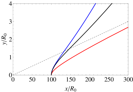
Figure 1: The shape of photospheres of a steady coasting relativistic wind (blue curve) and a steady accelerating relativistic wind (black curve) as well as the time-integrated photosphere of an infinitely thin shell (red curve) for $\Gamma=100$. The dashed line shows the relativistic beaming angle.

Secondly, the photosphere of a steady accelerating relativistic wind is described by a cubic equation. It corresponds to a static surface with curvature larger than that of the coasting wind, see Fig. 1. Thirdly, the photosphere of an infinitely thin shell at a fixed laboratory time within the relativistic beaming cone $\theta=\arccos\left(1-\frac{1}{2\eta^{2}}\right)$ is an infinitely thin ring. The collection of such rings for all laboratory times represents a surface given by

$$\frac{r}{R_{0}}=\left[{\tau_{0}\frac{1-\left(1-\frac{1}{2\eta^{2}}\right)\cos\theta}{|\cos\theta-\left(1-\frac{1}{2\eta^{2}}\right)|}}\right]^{1/2}.$$ (16)

The curvature of this surface is even larger than that of an accelerating wind, as can be seen from Fig. 1. This surface represents the asymptotic limit of photospheres of photon thin outflows. The surfaces (15) and (16) give the position of the corresponding photon thick and photon thin outflow photospheres with very good accuracy.

3 Radiative diffusion

The definition of the photosphere implies that at this position in space the outflow as a whole becomes transparent to radiation. However, emission emerges from the outflow when it is optically thick as well. Such emission is due to radiative diffusion which transfers the energy from deeper parts of the outflow towards its surface. Naively one can think that such an effect is negligible in ultrarelativistic outflows. However, this is not the case. This effect, usually neglected in the literature based on considerations of steady winds, plays a crucial role in photon thin outflows [28]. Actually, near the photosphere, photons are not produced in the outflow since three-particle interactions such as bremsstrahlung and double Compton scattering become inefficient (freeze out) at smaller radii. Hence photons may diffuse from the interior of the outflow to the boundary and eventually escape before the outflow reaches the photospheric radius. In such a case there will be no emission at the photospheric radius, since most photons have already escaped. This is exactly the case for photon thin outflows, as we will see below.

Consider the diffusion crossing time on which a photon is expected to cross the outflow with comoving radial thickness $l_{c}=\Gamma l$. This time is given by $t_{D,c}=l_{c}^{2}/D_{c}$, where the diffusion coefficient is $D_{c}=(c\lambda_{c})/3=c/(3\sigma n_{c})$ and $\lambda_{c}$ and $n_{c}$ are the comoving mean free path of photons and the comoving electron number density, respectively. One may find the radial position $R_{D}$ at which the outflow arrives by the time $t_{D,c}$. At this time, measured from the beginning of the expansion, photons actually cross the entire width of the outflow by diffusion. Neglecting the initial brief acceleration phase when diffusion is irrelevant, from the equation of motion of the outflow $R=\beta ct\simeq\Gamma ct_{c}$, where $t_{c}$ is time measured in comoving frame, and taking into account Eq. (7) we obtain

$$R_{D}=\left(\tau_{0}\eta^{2}R_{0}l^{2}\right)^{1/3}.$$ (17)

This diffusion radius should be compared to the photospheric radius (6). From the last line in Eq. (6) one finds

$$\frac{R_{D}}{R_{ph}}=\left(\frac{\eta^{4}l}{\tau_{0}R_{0}}\right)^{\frac{1}{6}},$$ (18)

which is valid for any acceleration model of the outflow.

For photon thick outflows one has $4\eta^{4}l\gg\tau_{0}R_{0}$ and the diffusion radius is always larger than the photospheric radius. In other words, the width of the outflow is so large that photons have no time to diffuse out by the moment the outflow becomes transparent. Hence diffusion is irrelevant for photon thick outflows.

The situation is the opposite for photon thin outflows, when $\tau_{0}R_{0}\gg 4\eta^{4}l$ and the diffusion radius is always smaller than the photospheric radius. This implies that in photon thin outflows radiation decouples not at the photospheric radius, defined by Eq. (6), but at the diffusion radius defined by Eq. (17), when the expanding plasma is still opaque. In this sense the characteristic radius of the photospheric emission from photon thin outflows is the diffusion radius.

4 Probability density

One has to keep in mind that photons decouple from the plasma not only at a surface given for photon thick outflows by the condition $\tau=1$. The last scattering of photons occurs in a finite region of spacetime near this surface. Hence the photosphere is not a sharp surface, but it is “fuzzy” [35, 13]. Since the outflow is dynamical and finite in spatial extension, the finiteness effects are expected to play an important role for the formation of the photospheric emission. Such effects have been recently investigated [36] by means of Monte Carlo simulations using the model of a relativistic wind with finite duration and considering both coherent and Compton scattering of photons.

Most of energy reaching an observer is emitted from the region near the photosphere, where the probability density function along the ray reaches its maximum. This function [28] is given by

$$P(r,\theta,t)\propto\frac{d}{ds}\exp[-\tau(r,\theta,t)],$$ (19)

where $s$ is the distance measured along the light-like world line. When the time dependence in this equation is discarded, this $P(r,\theta)$ coincides with the probability density function of the last scattering defined in Ref. 2008ApJ…682..463P.

The probability density of the photon last scattering position is shown in Fig. 2 as a function of the depth $\xi$ measured from the outer boundary of the outflow (top panel) and as a function of the radial coordinate (bottom panel). In photon thick outflows the photon decoupling is local and almost independent of $\xi$ (solid curve in the top panel of Fig. 2). Instead, this probability density depends strongly on the radial coordinate (curves 1–3 in the bottom panel of 2). The probability density function of last scattering is found to be close to the one of an infinite steady wind studied in Ref. 2011ApJ…737…68B. The difference emerges due to the presence of boundaries, and it is manifested in an exponential cut off in the probability density at large radii.

In photon thin outflows there is enough time for photons to be transported to the boundaries by diffusion as discussed above, see also Ref. 2013ApJ…772…11R. As a result the probability density as a function of the depth peaks at the boundaries (dashed curve in the top panel of Fig. 2).

Figure 2: Upper panel: Probability density of last scattering as a function of the normalized depth for photon thick and photon thin outflows (in the latter case decreased by a factor of 10 for a better presentation).
Lower panel: probability density function for the position of last scattering in the following cases: infinite and steady wind (1), photon thick case with $\Gamma=500$ (2), photon thick case with a smaller Lorentz factor $\Gamma=300$ (3), and photon thin outflow (4). The vertical line (a) represents the diffusion radius in the photon thin case, line (b) represents the photospheric radius while lines (c) and (d) show the transition radius $R_{t}=\eta R_{0}$ for curves (2) and (3), respectively.
Reproduced from Ref. 2013ApJ…767..139B.

It is also clear (see curve 4 in the bottom panel of 2) that most photons escape from the photon thin outflow well before the photospheric radius, namely near diffusion radius defined in Eq. (17). This result confirms that radiation diffusion plays an important role for this type of outflow. It actually determines the shape of both the instantaneous and time integrated spectra as seen by a distant observer, as well as the light curve [28].

5 Average number of scatterings

Another difference between the photon thick and photon thin cases manifests itself in the average number of scatterings as a function of the initial optical depth [36]. The average number of scatterings is defined as

$$\langle N\rangle=\int_{t_{i}}^{t_{f}}\frac{cdt_{c}}{\lambda_{c}}=\int_{t_{i}}^{t_{f}}\sigma\langle n_{c}\rangle cdt_{c},$$ (20)

where $t_{c}$ is the comoving time, $\lambda=1/(\sigma_{T}n_{c})$ is the comoving mean free path of photons, $n_{c}$ is the comoving density, $t_{i}$ is the initial comoving time, and $t_{f}$ is the final comoving time when the photon leaves the outflow. The integral (20) is taken along the average photon path. In an optically thick medium when diffusion is neglected, this path is given by the equation of motion of the outflow

$$r=r_{i}+\beta ct,$$ (21)

where $r_{i}$ is the laboratory radial position of the photon at the initial laboratory time. In the photon thick case photons stay in the outflow long after decoupling, so one can set $t_{f}\rightarrow\infty$. Then, taking into account relations $n_{c}=n_{l}/\Gamma$, $dr=\beta cdt$, and $t_{c}=t/\Gamma$ along the world line (21), we obtain

$$\langle N\rangle=\int_{t_{i}}^{\infty}\sigma\frac{n}{\Gamma}\frac{cdt}{\Gamma}=2\tau_{i},$$ (22)

where $\tau_{i}$ is optical depth of the outflow at $r_{i}$.

In the photon thin case the photons decouple from the outflow near its boundaries, and the time interval needed for the photon to reach them by a random walk can be estimated as $t^{c}_{D}=l_{c}^{2}/D_{c}$, where $l_{c}=\Gamma l$ is the comoving radial thickness of the outflow, and the diffusion coefficient is $D_{c}=(c\lambda_{c})/3=c/(3\sigma n_{c})$. When this time is much less than the characteristic time of expansion, equal to $t_{i}$, which is the case when the initial radius $r_{i}$ is much larger than radius of diffusion $R_{D}$, we have

$$\langle N\rangle\simeq 3\tau_{i}^{2},$$ (23)

In the opposite case when initial radius $r_{i}$ is much smaller than the radius of diffusion $R_{D}$, we have

$$\langle N\rangle\simeq\frac{1}{\Gamma^{2}}\sqrt{\tau_{i}\tau_{0}\frac{R_{0}}{l}}.$$ (24)

Figure 3: Average number of scatterings as function of initial optical depth $\tau_{i}$. Results of Monte Carlo simulations are shown with points, while analytic results are shown by the corresponding lines. In the optically thin regime the number of scatterings is proportional to $\tau_{i}$. For $1<\tau_{i}<\tau(R_{D})$ it is proportional to $\tau_{i}^{2}$. For $\tau(R_{D})<\tau_{i}<\tau(R_{t})$ it is proportional to $\tau_{i}^{1/2}$. For even larger $\tau_{i}$ corresponding to the photon thick asymptotic the number of scatterings is again proportional to $\tau_{i}$. In these simulations $\Gamma=100$, $l=10^{8}$ cm and $\tau_{0}=10^{14}$. Reproduced from Ref. 2013ApJ…767..139B.

The average number of scatterings in all these cases is shown in Fig. 3, together with the results of Monte Carlo simulations. Indeed, when the outflow is photon thick we have $\langle N\rangle\propto\tau_{i}$. This result is in contrast with a static optically thick finite medium [48] where $\langle N\rangle\propto\tau_{i}^{2}$. However, in photon thin outflows the number of scatterings is increasing with $\tau_{i}$ even more slowly, namely as $\langle N\rangle\propto\tau_{i}^{1/2}$ for most of the photons. Instead, for those photons which scatter at sufficiently large radii, larger than the diffusion radius, we have $\langle N\rangle\propto\tau_{i}^{2}$ as in the static medium. These photons arrive in the tail of the light curve.

These results have important implications in dissipative models of GRBs where either kinetic or electromagnetic energy gets converted into thermal energy of the outflow when it is still optically thick. They imply in particular that in contrast with a static medium, in a relativistically moving medium the spectral distortion is harder to achieve, since the number of scatterings is less in the latter case.

6 Laboratory time versus arrival time pictures

Once the photospheric radius (or diffusion radius) is known such averaged properties of the photospheric emission as the peak energy in the observed spectrum and the duration of emission can be determined. In order to know the detailed light curve and time resolved spectra one has to define the notion of a dynamic photosphere. Such a dynamic photosphere is determined in general by the condition $\tau(r,t,\theta)=1$. For an outflow with finite spatial extension this dynamic photosphere is located inside it and typically crosses the outflow from the outer to the inner boundary while the total optical depth of the outflow defined by Eq. (2) decreases to unity.

It is well known that the optical depth is a Lorentz invariant quantity, for relevant discussion see Ref. Siutsou2013. However, due to relativistic motion the picture of the dynamic photosphere in relativistic outflow looks different in the laboratory and observer reference frames. A distant observer uses the arrival time $t_{a}$ which is related to the laboratory time $t$, the radial coordinate $r$ and the angle $\theta$ measured in the laboratory frame as

$$t_{a}=t-r\cos\theta/c.$$ (25)

Hence photons emitted at one and the same laboratory time but from points with different $\theta$ are detected at different arrival times; vice versa, photons detected at the same values of the arrival time have been emitted at different laboratory times and from points with different $\theta$. At a given arrival time one has an “equitemporal surface”, see e.g., Ref. 2001A&A…368..377B, i.e., the surface locus of points emitting photons with the same value of the arrival time $t_{a}$. The corresponding equitemporal surface of the photospheric emission is referred to as the PhE surface[28].

Given the hydrodynamic profiles of the number density of electrons $n(r,t)$ and the Lorentz factor $\Gamma(r,t)$ of the spherically symmetric outflow, one can compute the optical depth and find the surface corresponding to the condition $\tau(r,t,\theta)=1$. For the simplest case of a relativistic wind with finite duration there is only one such surface at a given laboratory time $t$. In general, however, for a single peaked density profile there are two surfaces: the outer photosphere and the inner one, see e.g., Ref. Begue2013. The inner photosphere appears because of two opposite effects: the increase of density with decreasing depth, and the decrease of density due to expansion. For the outer photosphere both effects work in the same direction.

The distant observer, however, can see only one photosphere at a given arrival time, namely the PhE surface. For a single peaked density profile the light curve seen by this observer will be also single peaked. Emission originating from the outer photosphere arrives first. The peak in the light curve corresponds roughly to emission from the peak in the laboratory density profile. Emission from the inner photosphere arrives in the tail of the light curve.

For more complex hydrodynamic profiles with multiple peaks in the electron number density, multiple photospheres may appear, which may result in a spiky light curve of the photospheric emission with a variable time scale down to $R_{0}/c$, i.e., milliseconds [40]. In this respect observations may be used for reconstruction of the underlying hydrodynamic profiles, see Ref. 2013MNRAS.433.2739I. In addition, departure from spherical symmetry manifested in the appearance of an angular dependence of hydrodynamic quantities, in particular of the bulk Lorentz factor, is also crucial for the formation of observed spectra of photospheric emission [41].

7 Spectra and light curves as seen by a distant observer

Several methods of computing the spectra and light curves of photospheric emission as seen by a distant observer have been proposed, in particular: integration over the PhE surface [42, 28]; integration over volume with attenuation factors [12, 41]; approximations to the radiative transfer [13, 28]; Monte Carlo simulations of photon scattering [16, 43, 36, 44]; Fokker-Planck approximation to the collision integral with an anisotropic photon field (generalized Kompaneets equation) [19] and relativistic Boltzmann equations [45, 46]. It is remarkable that several very different methods produce practically the same results, see Fig. 4.

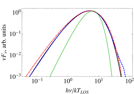
Figure 4: The spectrum of photospheric emission from photon thick outflow obtained with different approximations, but with the same parameters of the outflow. The dotted curve shows the Planck spectrum. The dashed-dotted curve shows the result from Ref. 2013ApJ…772…11R obtained using the fuzzy photosphere approximation. The dotted curve shows the result from Ref. 2013ApJ…767..139B obtained from Monte Carlo simulations. The solid curve shows the result from Ref. 2013MNRAS.tmpL.153A obtained by the solution of the radiative transfer equation with the Fokker-Planck approximation to the collision integral.

All these results indicate that the photospheric spectrum is wider than the Planck one. There is an increase in the low energy slope of the spectrum, resulting in the photon index $\alpha\simeq 0$, in contrast with the Planck photon index $\alpha=1$.

The computation method based on the radiative transfer equation turns out to be useful since it represents a second step beyond the simplest approach adopted by Goodman [6]. In fact, for estimating the observed spectrum Goodman used superpositions of Planck spectra corresponding to different emitting regions with temperatures obtained from hydrodynamic equations. In approximate solutions of the radiative transfer equations using “fuzzy photosphere” and “sharp photosphere” approximations [28] the spectrum coming from a given region no longer has the Planck shape, although the source function in the comoving frame is still assumed to be isotropic and thermal. Even if the approximations adopted in this approach are plausible and consistent, they must be verified by different methods.

Monte Carlo simulation is a completely independent method. Here each photon is followed in the laboratory reference frame where the plasma is initially at rest while it experiences numerous collisions with the cross sections of Compton and isotropic scattering models, until it ceases scattering. Photons are injected in the expanding plasma well before it becomes transparent.The resulting photons constitute the final spectrum. The drawbacks of this approach are: a prescribed distribution of an electron component and the impossibility to account for the stimulated emission of photons. The possibility to take into account Pauli blocking in Monte Carlo simulations of degenerate relativistic plasmas has recently been discussed in Ref. 2013JCoPh.249…13T. The first limitation originates from the fact that Monte Carlo simulations need a prescribed background of electrons, and any back-reaction of photons on the electron distribution can be only accounted for by an iterative scheme. The second limitation constrains the spectrum of photons in the optically thick region to have a Wien shape instead of the Planck one, if the model of Compton scattering is used. In addition, the good statistics required to resolve both the low and high energy parts of the photon spectrum imply the need for a large number of photons which in turn demands long computational times.

The Fokker-Planck approximation to the Boltzmann equation allows one to take into account the stimulated emission of photons. However, it does not allow accounting for variations in the distribution function of the electron component. In this approach which solves partial differential equations, a rather good resolution in the spectrum can be achieved. In the recent study [19] the formation of the spectrum from the photospheric emission in relativistic winds is analyzed with this method. The comoving temperature is assumed to depend on the laboratory radius as $T\propto r^{-k}$, where $k=2/3$ corresponds to the law of adiabatic expansion of the relativistic coasting wind. The low energy power law index $\alpha$ of the observed spectrum is found to be a function of the power law index $k$ in the temperature distribution as $\alpha\simeq 1-k$.

Finally, numerical solution of the system of Boltzmann equations for electrons and photons is the most promising method. Here Compton scattering of photons is followed from high optical depth regions to low optical depth ones, and the complete evolution of both the photon and electron distributions can be obtained self-consistently. Since finite difference methods are involved, the only limitation in this approach is the size of the grid in the phase space.

Next we give a short overview of methods suggested in Ref. 2013ApJ…772…11R. The basis of the spectrum and flux calculation is the radiative transfer equation for the specific intensity $I_{\nu}$ along the ray (see e.g., Ref. 1979rpa..book…..R)

$$\frac{dI_{\nu}}{ds}=j_{\nu}-\kappa_{\nu}I_{\nu},$$ (26)

where $j_{\nu}$ is the monochromatic emission coefficient for frequency $\nu$, $\kappa_{\nu}$ is the absorption coefficient and $s$ is the distance measured along the ray.

The spectral intensity of radiation measured at infinity from a ray coming to an observer at some arrival time $t_{a}$ is given by the formal solution of this equation [13]

$$I_{\nu}(\nu,\rho,t_{a}) =\int\mathcal{I}_{\nu}(\nu,r,\theta,t)\frac{d}{ds}\left\{\exp[-\tau(\nu,r,\theta,t)]\right\}\,ds$$ (27)

$$=\int\mathcal{I}_{\nu}(\nu,r,\theta,t)\exp[-\tau(\nu,r,\theta,t)]\,d\tau,$$

where $\mathcal{I}_{\nu}(r,\theta,t)$ is the source function, equal to the ratio of emission and absorption coefficients $\mathcal{I}_{\nu}=j_{\nu}/\kappa_{\nu}$, the optical depth $\tau$ is given by

$$\tau=\int_{s}^{\infty}\kappa_{\nu}ds,$$ (28)

coinciding with Eq. (1), and the variables $(r,\theta,t)$ are connected by Eq. (25) and $\rho=r\sin\theta$.

The total observed flux is an integral over all the rays

$$F_{\nu}(\nu,t_{a})=2\pi\Delta\Omega\int I_{\nu}(\nu,\rho,t_{a})\,\rho\,d\rho\,,$$ (29)

where $\Delta\Omega$ is the solid angle of the observer’s detector as seen from the outflow in the laboratory frame and $2\pi\rho d\rho$ is an element of area in the plane of the sky.

The emissivity $j_{\nu}$ is assumed to be thermal and isotropic in the comoving frame of the outflow and the comoving opacity is $\kappa_{\nu,c}=\mathrm{const}$. The laboratory source function is then

$$\mathcal{I}_{\nu}(\nu,r,\theta,t)=\frac{2h}{c^{2}}\frac{\nu^{3}}{\exp\left(\frac{h\nu\Gamma(1-\beta\cos\theta)}{kT_{c}(r,t)}\right)-1},$$ (30)

where $h$ is Planck’s constant. This approximation is justified when the radiation field is tightly coupled to the matter. The photospheric emission comes from the entire volume of the outflow, [38] and the computational method sketched above is closely related to that used in Ref. 2011ApJ…737…68B, where the concept of the “fuzzy photosphere” was introduced. This method is referred to as the fuzzy photosphere approximation.

Most of the energy reaching the observer is emitted from the region near the PhE surface, where the probability density function along the ray given by Eq. (19) reaches its maximum. For this reason the dynamics of the PhE surface discussed in the previous section determines both the light curves and spectra of the observed photospheric emission. Assuming that all the energy comes from the PhE surface only, i.e., a surface instead of the volume discussed above, the computation may be reduced to a one-dimensional integration by substitution of the function $P$ by a Dirac delta function. Such a cruder approximation, in contrast with the fuzzy photosphere one, is referred to as the sharp photosphere approximation.

8 Dissipative photospheres

In spite of the title this review, I conclude with a brief discussion of dissipative photospheric models of GRBs. All these models assume that some energy is eventually converted into photons in the optically thick regime, which makes the photospheric component brighter. In the literature such dissipation is associated with magnetic reconnection [49, 50, 15, 43], neutron decay [51, 52, 53, 54], collisional heating [16] and internal shocks [24, 55, 17].

Consider generic dissipation models following Ref. 2005ApJ…628..847R. When the kinetic energy of the outflow is dissipated, electron-positron pairs may be created and the pair photosphere where the optical depth of the outflow due to Compton scattering on pairs reaches unity may emerge. When continuous dissipation occurs in the steady coasting wind, the pair photosphere can be found from the balance between the rate of energy dissipation and the expansion rate $c\Gamma/r$. The former is given by $n_{\gamma}\sigma_{T}c$, where $n_{\gamma}=L/(4\pi r^{2}m_{e}c^{3}\Gamma^{2})$ is the comoving photon density, $m_{e}$ is the electron mass, $L=\epsilon L_{0}$ is the dissipated radiative luminosity in the observer frame, $L_{0}$ is the luminosity of the wind and $\epsilon$ is the efficiency parameter. Assuming that photons have sufficient energy to produce pairs one can obtain the photospheric radius of pairs produced by dissipation of energy as

$$R_{\pm,d}\lesssim\frac{L\sigma_{T}}{4\pi m_{e}c^{3}\Gamma^{2}}.$$ (31)

When compared to the second line in Eq. (6) we find $R_{\pm,d}\lesssim R_{ph}m_{p}/m_{e}$. This pair photosphere may be located beyond the baryonic one, thus changing the observed properties of the photospheric emission with respect to the case without dissipation.

Another interesting effect is that the baryonic photosphere is also moved further away after dissipation has occurred due to the decrease in the Lorentz factor. This may be important in a scenario with sudden dissipation at a certain radius above the saturation radius $\eta^{\frac{1}{a}}R_{0}$. When a sufficiently large fraction of the kinetic energy is converted back into thermal energy, the outflow may again become radiation-dominated and additional acceleration will occur. In this case photospheric emission will necessarily originate before the outflow starts to coast again. This means that impulsive strong dissipation may change the character of the photosphere.

Two particular scenarios were analyzed in Ref. 2006ApJ…642..995P: with slow heating [57] and with internal shock. While details of these scenarios vary, in both cases the role of dissipation is two-fold. Firstly, it converts a fraction of kinetic or electromagnetic energy of the outflow into thermal energy. Secondly, it is supposed to supply additional soft photons which may be Comptonized on the population of electrons accelerated or heated by the dissipation process. Numerical simulations performed in Ref. 2006ApJ…642..995P suggest that strong deviations from pure black body spectra are possible for various parameters of these models. In particular, when dissipation (e.g., shocks or heating) occur at high optical depths of the outflow, the observed spectrum is dominated by the Wien component which appears as result of Comptonization regardless of the values of the parameters in the models considered. For intermediate optical depths on the order of unity, multiple scattering creates the flat energy per decade spectrum above the peak. For lower optical depths the dissipation is ineffective in broadening the spectral component originating from the photosphere.

The basic feature of all photospheric models with dissipation is the possibility to further broaden the spectrum of the photospheric emission. Besides, the intensity of the photospheric emission gets amplified. These models manage to reproduce some observed features in GRB spectra, see e.g., Ref. 2011MNRAS.415.1663T,2011MNRAS.415.3693R. However, the need to produce a sufficient number of photons for thermalization implies strong constraints on the parameters of models involving dissipation, see e.g., Ref. 2012MNRAS.422.3092G,2013ApJ…764..143V. Moreover, so far there is no convincing dissipative model which on the one hand is based on a self-consistent relativistic hydrodynamics and/or kinetics, and on the other hand is able to reproduce many of the observational features of GRBs.

9 Discussion and conclusion

Photospheric emission is a natural ingredient of most popular models of GRBs such as the fireball, fireshell or electromagnetic models. Despite the fact that GRBs are not generally characterized by a Planck spectrum, recent observations demonstrate that subdominant thermal components are likely to be present in many bursts. This fact makes photospheric models of GRBs an attractive alternative to other models involving only optically thin emission mechanisms.

In this review I have discussed a number of different physical aspects, in particular relativistic effects, which make the photospheric emission from relativistic outflows an interesting subject to study. From this analysis it follows that the expectation that a relativistic photosphere produces a black body spectrum with a Lorentz boosted temperature is too naive. One can ask a general question: is there a way to distinguish between a static optically thick source emitting from its photosphere and a relativistically expanding one? It is the low energy part of the spectrum that holds the key to answering this question. The analysis performed so far implies that if the observational data are of sufficiently good quality in order to resolve the low energy part of the spectrum, the answer to this question is positive. As Fig. 4 clearly illustrates, the relativistically expanding source produces the spectrum with a low energy slope different from the Planck case. Possible dissipation near the photosphere may further broaden the observed spectrum and make it similar to the one observed in many GRBs.

The photosphere is likely not the only source of radiation responsible for producing GRB emission, see Ref. 2012ApJ…758L..34Z. Due to relativistic effects emission from the photosphere may arrive at the observer almost simultaneously with the optically thin emission [58, 61, 62]. What is crucial, however, is that photospheric emission carries unique information about basic physical parameters of the relativistic outflow producing the GRB.

Acknowledgement. I am indebted to Alexey Aksenov, Vladimir Belinski, Carlo Luciano Bianco, Remo Ruffini and She-Sheng Xue for discussions. I would also like to thank Damien Begue, Robert Jantzen, and Ivan Siutsou for a critical reading of the manuscript.

References

- [1] T. Piran, Phys. Rep. 314 (June 1999) 575.
- [2] R. Ruffini, M. G. Bernardini, C. L. Bianco, L. Caito, P. Chardonnet, M. G. Dainotti, F. Fraschetti, R. Guida, M. Rotondo, G. Vereshchagin, L. Vitagliano and S.-S. Xue, The Blackholic energy and the canonical Gamma-Ray Burst, in American Institute of Physics Conference Series, , American Institute of Physics Conference Series Vol. 910 (June 2007), pp. 55–217.
- [3] D. Band, J. Matteson, L. Ford, B. Schaefer, D. Palmer, B. Teegarden, T. Cline, M. Briggs, W. Paciesas, G. Pendleton, G. Fishman, C. Kouveliotou, C. Meegan, R. Wilson and P. Lestrade, ApJ 413 (August 1993) 281.
- [4] G. Vianello, Fermi GRB spectra and the crisis of the Band model, in Proceedings of the Thirteenth Marcel Grossman Meeting on General Relativity, eds. K. Rosquist, R. Jantzen and R. Ruffini (World Scientific, Singapore, 2013).
- [5] S. Guiriec, F. Daigne, R. Hascoët, G. Vianello, F. Ryde, R. Mochkovitch, C. Kouveliotou, S. Xiong, P. N. Bhat, S. Foley, D. Gruber, J. M. Burgess, S. McGlynn, J. McEnery and N. Gehrels, ApJ 770 (June 2013) 32, arXiv:1210.7252 [astro-ph.HE].
- [6] J. Goodman, ApJ 308 (September 1986) L47.
- [7] B. Paczynski, ApJ 308 (September 1986) L43.
- [8] B. Paczynski, ApJ 363 (November 1990) 218.
- [9] R. Ruffini, J. D. Salmonson, J. R. Wilson and S.-S. Xue, A&A 359 (July 2000) 855.
- [10] R. D. Preece, M. S. Briggs, R. S. Mallozzi, G. N. Pendleton, W. S. Paciesas and D. L. Band, ApJ 506 (October 1998) L23, arXiv:astro-ph/9808184.
- [11] A. Pe’er, Theory of photospheric emission in Gamma-Ray Bursts, in Proceedings of the Thirteenth Marcel Grossman Meeting on General Relativity, eds. K. Rosquist, R. Jantzen and R. Ruffini (World Scientific, Singapore, 2013).
- [12] A. Pe’er and F. Ryde, ApJ 732 (May 2011) 49.
- [13] A. M. Beloborodov, ApJ 737 (August 2011) 68, arXiv:1011.6005 [astro-ph.HE].
- [14] S. Dodelson, Modern cosmology 2003.
- [15] D. Giannios, A&A 457 (October 2006) 763, arXiv:astro-ph/0602397.
- [16] A. M. Beloborodov, MNRAS 407 (September 2010) 1033, arXiv:0907.0732 [astro-ph.HE].
- [17] K. Toma, X.-F. Wu and P. Mészáros, MNRAS 415 (August 2011) 1663, arXiv:1002.2634 [astro-ph.HE].
- [18] D. Lazzati, B. J. Morsony, R. Margutti and M. C. Begelman, ApJ 765 (March 2013) 103, arXiv:1301.3920 [astro-ph.HE].
- [19] A. G. Aksenov, R. Ruffini and G. V. Vereshchagin, MNRAS (August 2013) arXiv:1308.1848 [astro-ph.HE].
- [20] A. Pe’er, F. Ryde, R. A. M. J. Wijers, P. Mészáros and M. J. Rees, ApJ 664 (July 2007) L1, arXiv:astro-ph/0703734.
- [21] S. Iyyani, F. Ryde, M. Axelsson, J. M. Burgess, S. Guiriec, J. Larsson, C. Lundman, E. Moretti, S. McGlynn, T. Nymark and K. Rosquist, MNRAS 433 (August 2013) 2739, arXiv:1305.3611 [astro-ph.HE].
- [22] J. Ehlers, Survey of general relativity theory, in Relativity, Astrophysics and Cosmology, (1973), pp. 1–125.
- [23] M. A. Abramowicz, I. D. Novikov and B. Paczynski, ApJ 369 (March 1991) 175.
- [24] F. Daigne and R. Mochkovitch, MNRAS 336 (November 2002) 1271, arXiv:astro-ph/0207456.
- [25] P. Mészáros and M. J. Rees, ApJ 733 (June 2011) L40, arXiv:1104.5025 [astro-ph.HE].
- [26] P. Veres, B.-B. Zhang and P. Mészáros, ApJ 764 (February 2013) 94, arXiv:1210.7811 [astro-ph.HE].
- [27] A. Shemi and T. Piran, ApJ 365 (December 1990) L55.
- [28] R. Ruffini, I. A. Siutsou and G. V. Vereshchagin, ApJ 772 (July 2013) 11, arXiv:1110.0407 [astro-ph.CO].
- [29] A. G. Aksenov, R. Ruffini and G. V. Vereshchagin, Thermalization of Electron-Positron-Photon Plasmas with an application to GRB, in American Institute of Physics Conference Series, , American Institute of Physics Conference Series Vol. 966 (January 2008), pp. 191–196.
- [30] R. Ruffini and G. Vereshchagin, Il Nuovo Cimento C 36 (May 2013) 255, arXiv:1205.3512 [astro-ph.CO].
- [31] G. S. Bisnovatyi-Kogan and M. V. A. Murzina, Phys. Rev. D 52 (October 1995) 4380.
- [32] T. Piran, A. Shemi and R. Narayan, MNRAS 263 (August 1993) 861.
- [33] P. Mészáros, P. Laguna and M. J. Rees, ApJ 415 (September 1993) 181.
- [34] R. Ruffini, I. A. Siutsou and G. V. Vereshchagin, New A 27 (2014) 30, arXiv:1309.3857 [astro-ph.HE].
- [35] A. Pe’er, ApJ 682 (July 2008) 463, arXiv:0802.0725.
- [36] D. Bégué, I. A. Siutsou and G. V. Vereshchagin, ApJ 767 (April 2013) 139, arXiv:1302.4456 [astro-ph.HE].
- [37] I. A. Siutsou, Relativistic plasma and transparency in Gamma-Ray Bursts and equilibrium self-gravitating systems of fermions, PhD thesis, International Relativistic Astrophysics PhD (2013).
- [38] C. L. Bianco, R. Ruffini and S. Xue, A&A 368 (March 2001) 377, arXiv:astro-ph/0102060.
- [39] D. Bégué and G. V. Vereshchagin, MNRAS, submitted (2013).
- [40] M. J. Rees and P. Mészáros, ApJ 628 (August 2005) 847, arXiv:astro-ph/0412702.
- [41] C. Lundman, A. Pe’er and F. Ryde, MNRAS 428 (January 2013) 2430, arXiv:1208.2965 [astro-ph.HE].
- [42] A. Mizuta, S. Nagataki and J. Aoi, ApJ 732 (May 2011) 26, arXiv:1006.2440 [astro-ph.HE].
- [43] D. Giannios, MNRAS 422 (June 2012) 3092, arXiv:1111.4258 [astro-ph.HE].
- [44] H. Ito, S. Nagataki, M. Ono, S.-H. Lee, J. Mao, S. Yamada, A. Pe’er, A. Mizuta and S. Harikae, ArXiv e-prints (June 2013) arXiv:1306.4822 [astro-ph.HE].
- [45] A. Pe’er and E. Waxman, ApJ 628 (August 2005) 857, arXiv:astro-ph/0409539.
- [46] A. Benedetti and G. V. Vereshchagin, ApJ, to be submitted (2013).
- [47] A. E. Turrell, M. Sherlock and S. J. Rose, Journal of Computational Physics 249 (September 2013) 13.
- [48] G. B. Rybicki and A. P. Lightman, Radiative processes in astrophysics 1979.
- [49] C. Thompson, MNRAS 270 (October 1994) 480.
- [50] D. Giannios and H. C. Spruit, A&A 430 (January 2005) 1, arXiv:astro-ph/0401109.
- [51] E. V. Derishev, V. V. Kocharovsky and V. V. Kocharovsky, ApJ 521 (August 1999) 640.
- [52] A. M. Beloborodov, ApJ 585 (March 2003) L19, arXiv:astro-ph/0209228.
- [53] E. M. Rossi, A. M. Beloborodov and M. J. Rees, MNRAS 369 (July 2006) 1797, arXiv:astro-ph/0512495.
- [54] H. B. J. Koers and D. Giannios, A&A 471 (August 2007) 395, arXiv:astro-ph/0703719.
- [55] D. Lazzati and M. C. Begelman, ApJ 725 (December 2010) 1137, arXiv:1005.4704 [astro-ph.HE].
- [56] A. Pe’er, P. Mészáros and M. J. Rees, ApJ 642 (May 2006) 995, arXiv:astro-ph/0510114.
- [57] G. Ghisellini and A. Celotti, ApJ 511 (February 1999) L93, arXiv:astro-ph/9812079.
- [58] F. Ryde, A. Pe’Er, T. Nymark, M. Axelsson, E. Moretti, C. Lundman, M. Battelino, E. Bissaldi, J. Chiang, M. S. Jackson, S. Larsson, F. Longo, S. McGlynn and N. Omodei, MNRAS 415 (August 2011) 3693, arXiv:1103.0708 [astro-ph.HE].
- [59] I. Vurm, Y. Lyubarsky and T. Piran, ApJ 764 (February 2013) 143, arXiv:1209.0763 [astro-ph.HE].
- [60] B. Zhang, R.-J. Lu, E.-W. Liang and X.-F. Wu, ApJ 758 (October 2012) L34, arXiv:1208.1812 [astro-ph.HE].
- [61] A. Pe’er, B.-B. Zhang, F. Ryde, S. McGlynn, B. Zhang, R. D. Preece and C. Kouveliotou, MNRAS 420 (February 2012) 468, arXiv:1007.2228 [astro-ph.HE].
- [62] M. Muccino, R. Ruffini, C. L. Bianco, L. Izzo and A. V. Penacchioni, ApJ 763 (February 2013) 125, arXiv:1205.6600 [astro-ph.HE].