Log-Periodic Oscillations in the Photo Response of Efimov Trimers

Abstract

The photoassociation of Efimov trimer, composed of three identical bosons, is studied utilizing the multipole expansion. For identical particles the leading contribution comes from the $r^{2}$ $s$-mode operator and from the quadrupole $d$-mode operator. Log-periodic oscillations are found in the photoassociation response function, both near the energy threshold for the leading $s$-wave reaction, and in the high frequency tail for all partial waves.

I Introduction

The implementation of photo-association techniques in ultracold atomic traps Thompson et al (2005) opened a new route for quantitative determination of universal properties in few-body systems Braaten and Hammer (2006). In these experiments, radio-frequency (rf) induced trimer formation leads to enhanced atom loss rates from the traps. Scanning the rf field frequency, the change in the measured atom loss rate indicates various molecular thresholds and structures.

Recently, trimer formation through rf association was discovered in both fermionic ⁶Li Lompe et al (2010); Nakajima et al (2011) and bosonic ⁷Li Machtey et al (2012) systems. The three body case attracts special attention as the simplest non-trivial system. Moreover, in the 70’s Efimov predicted that in the limit of a resonant 2-body interaction, the system reveals universal properties Efimov (1970). A peculiar prediction is the existence of a series of giant three body molecules, known as Efimov trimers, that was verified experimentally few years ago Zaccanti et al (2009); Pollack et al (2009); Gross et al (2009, 2011).

In a previous work Bazak et al (2012), we have presented the multipole analysis of an rf association process binding a molecule of $N$ identical bosons. We have shown that the spin-flip and frozen-spin processes differ by their operator structure and by the de-excitation modes that contribute to the photoassociation rate. Previous analysis of these rf experiments Chin and Julienne (2005); Bertelsen and Mølmer (2006); Hanna et al (2007); Klempt et al (2008); Tscherbul and Rittenhouse (2011), which relied on the Franck-Condon factor, is appropriate for describing spin-flip reactions. For frozen-spin reactions we have applied our results to study the dimer formation Bazak et al (2012), and to study numerically the quadrupole response of a bound bosonic trimer Liverts et al (2012); Bazak et al (2013).

Here, we study trimer photoassociation using the hyperspherical adiabatic approximation. A zero-range potential is used to derive analytic results for the transition rates at the unitary point. Similarly to the dimer case Bazak et al (2012), the $s$-mode and the $d$-mode are found to be the leading order contributions. A new fingerprint of Efimov physics is studied, which is a log-periodic oscillation in the response.

II Multipole expansion

The molecular photoassosiaction rate is given by Fermi’s golden rule,

$$r_{i\rightarrow f}=\frac{2\pi}{\hbar}\bar{\sum_{i}}\sum_{f}|\langle f,\boldsymbol{k}\zeta|\hat{H}_{I}|i\rangle|^{2}\delta(E_{i}-E_{f}-\hbar\omega_{k})\;,$$ (1)

where three particles in an initial continuum state with energy $E_{i}$ form a bound state with energy $E_{f}$ by emitting a photon with momentum $\boldsymbol{k}$, polarization $\zeta$ and energy $\hbar\omega_{k}=\hbar ck$. $\bar{\sum}_{i}$ is an average on the appropriate initial continuum states and $\sum_{f}$ is a sum on the final bound states. The coupling between the neutral atoms and the radiation field takes the form $\hat{H}_{I}=-e\int d\boldsymbol{x}\;\boldsymbol{\mu}(\boldsymbol{x})\cdot\nabla\times\boldsymbol{A}(\boldsymbol{x})$, where $\boldsymbol{A}$ is the electromagnetic (EM) photon field, and $\mu(\boldsymbol{x})$ is the magnetization current. Here we consider only the one-body current $\mu(\boldsymbol{x})=\mu_{0}\sum_{j}\boldsymbol{S}_{j}\delta(\boldsymbol{x}-\boldsymbol{r}_{j})$, where $\mu_{0}$ is the magnetic moment of a single particle, and $\boldsymbol{S}_{j}$ and $\boldsymbol{r}_{j}$ are the spin and position of particle $j$.

We assume that the initial and final atomic wave functions can be written as a product of symmetric spin $|\chi\rangle$ and configuration space $|\psi\rangle$ terms, and that the photon does not induce change in the spin structure of the system. In this case the transition matrix element can be written as

$$\langle f,\boldsymbol{k}\zeta|\hat{H}_{I}|i\rangle=-i\mu_{0}\sqrt{\frac{\hbar c^{2}}{2{\cal V}\omega_{k}}}k\langle S_{0}\rangle\langle\psi^{f}_{L^{\prime}M^{\prime}}|\sum_{j=1}^{3}e^{i\boldsymbol{k}\cdot\boldsymbol{r}_{j}}|\psi^{i}_{LM}\rangle\;,$$ (2)

where $\langle S_{0}\rangle=\frac{1}{3}\sum_{j}\langle\chi^{i}_{M_{F}}|S_{j,0}|\chi^{i}_{M_{F}}\rangle$ is the average single particle magnetic moment, which plays the role of an effective charge. We normalize the EM field in a box of volume ${\cal V}$.

The photon wavelength of rf radiation is much larger than the typical dimension of the system $R$, therefore $kR\ll 1$ and the lowest order in $kR$ dominates the interaction. Therefore the exponent can be expanded to get

$$\sum_{j=1}^{3}e^{i\boldsymbol{k}\cdot\boldsymbol{r}_{j}}\approx 3+i\sum_{j=1}^{3}\boldsymbol{k}\cdot\boldsymbol{r}_{j}-\frac{1}{6}\sum_{j=1}^{3}k^{2}r_{j}^{2}-\frac{4\pi}{15}\sum_{j=1}^{3}k^{2}r_{j}^{2}\sum_{m}Y_{2-m}(\hat{k})Y_{2m}(\hat{r}_{j}),$$ (3)

where $Y_{lm}$ are the spherical harmonics. Each order in this expansion has clear physical meaning. The zeroth order operator stands for elastic interaction. The first order operator is the dipole, which for identical particles is proportional to the center of mass and hence does not affect the relative motion of the atoms. At second order two operators appear: the $r^{2}$ operator, corresponding to $s$-mode reaction, and the quadrupole terms, corresponding to $d$-mode reaction. For identical particles this is the leading term in low energy frozen spin reactions, and the transition probability scales as $k^{5}$. Summing over the initial and final magnetic numbers $M$, $M^{\prime}$, the transition matrix element reads

$$\sum_{M,M^{\prime}}|\langle f,\boldsymbol{k}\zeta|\hat{H}_{I}|i\rangle|^{2}=\frac{4\pi\hbar ck^{5}\mu_{0}^{2}}{2\Omega}\left|\left\langle S_{0}\right\rangle\right|^{2}\left(\frac{1}{6^{2}}|\langle\psi^{f}_{L^{\prime}}\|\sum_{j=1}^{3}r_{j}^{2}Y_{0}\|\psi^{i}_{L}\rangle|^{2}+\frac{1}{15^{2}}|\langle\psi^{f}_{L^{\prime}}\|\sum_{j=1}^{3}r_{j}^{2}Y_{2}(\hat{r}_{j})\|\psi^{i}_{L}\rangle|^{2}\right).$$ (4)

III The Three Body Problem

The dynamics of a quantum 3 particle system is governed by the Schroedinger equation

$$\left(T+W\right)\psi=E\psi$$ (5)

where $T$ is the center of mass kinetic energy operator and $W$ is the potential. In this study we shall limit our attention to short range 2-body forces, thus $W=\sum_{i<j}V(|\boldsymbol{r}_{i}-\boldsymbol{r}_{j}|)$. To eliminate the center of mass motion, we define the Jacobi coordinates, $\boldsymbol{x}=\sqrt{\frac{1}{2}}(\boldsymbol{r}_{2}-\boldsymbol{r}_{1})$, and $\boldsymbol{y}=\sqrt{\frac{2}{3}}\left(-\boldsymbol{r}_{3}+\frac{\boldsymbol{r}_{1}+\boldsymbol{r}_{2}}{2}\right)$, which we transform into the hyperspherical coordinates $\rho^{2}=x^{2}+y^{2}$, and $\Omega=(\alpha,\hat{x},\hat{y})$, where $\tan\alpha=x/y$.

In the limit of infinite scattering length, $|a|\rightarrow\infty$, the spatial wave function can be written as Macek (1968) $\psi(\rho,\Omega)=\rho^{-5/2}\mathcal{R}(\rho)\Phi(\Omega)$. The hyperspherical functions $\Phi(\Omega)$ and the corresponding eigenvalue $\nu^{2}$, are the solutions of the hyperangular equation,

$$\left(\hat{K}^{2}+\frac{2m\rho^{2}}{\hbar^{2}}\sum_{i}V(\sqrt{2}\rho\sin\alpha_{i})+4\right)\Phi=\nu^{2}\Phi,$$ (6)

where $\hat{K}^{2}=-\frac{1}{\sin 2\alpha}\frac{\partial^{2}}{\partial\alpha^{2}}\sin 2\alpha+\frac{\hat{l}^{2}_{x}}{\sin^{2}\alpha}+\frac{\hat{l}^{2}_{y}}{\cos^{2}\alpha}-4.$ For low energy physics, when the extension of the wave function is much larger than the range of the potential, one can utilize the zero range approximation. In this approximation the lateral extension of the potential is neglected all together, and the action of the potential is represented through the appropriate boundary conditions. For a two-particle system the low energy interaction is dominated by the $s$-wave scattering length $a$ and the wave function fulfills the boundary condition $[u^{\prime}/u]_{r=0}=-1/a$. The corresponding 3-body condition is

$$\left[\frac{1}{2\alpha\Phi}\frac{\partial}{\partial\alpha}2\alpha\Phi\right]_{\alpha=0}=-\sqrt{2}\frac{\rho}{a}\;.$$ (7)

Plugging the solution of Eq. (6) into Eq. (7), one gets transcendental equations for $\nu$. For $L=0$ the resulting equation is Fedorov and Jensen (2001)

$$\nu\cos(\nu\pi/2)-\frac{8}{\sqrt{3}}\sin(\nu\pi/6)=\frac{\sqrt{2}\rho}{a}\sin(\nu\pi/2).$$ (8)

For $|a|=\infty$ the solution with lowest $\nu^{2}$ is $\nu_{0}\approx 1.00624i$, corresponding to the Efimov trimer.

For $L=2$ the corresponding equation is,

$$\nu(4-\nu^{2})\cos(\nu\pi/2)+24\nu\cos(\nu\pi/6)+\frac{8}{\sqrt{3}}(\nu^{2}-10)\sin(\nu\pi/6)=-\frac{\rho}{a}(\nu^{2}-1)\sin(\nu\pi/2)$$ (9)

For $|a|=\infty$ the lowest non-trivial solution is $\nu_{2}\approx 2.82334$.

In the limit of $|a|\rightarrow\infty$, $\nu_{L}(\rho)=\nu_{L}$ and the hyperradial equation for $\mathcal{R}(\rho)$ is similar to the Bessel equation,

$$-\mathcal{R}^{\prime\prime}(\rho)+\frac{\nu_{L}^{2}-1/4}{\rho^{2}}\mathcal{R}(\rho)=\epsilon\mathcal{R}(\rho).$$ (10)

where $\epsilon=2mE/\hbar^{2}$.

We seek the solution for the bound ($\epsilon<0$) and continuum ($\epsilon>0$) cases:

I. A bound state exists only for $L=0$, and $\nu_{0}\approx 1.00624i$. In this case the relevant solution is $\sqrt{\rho}K_{\nu_{0}}(\kappa\rho)$, where $\kappa=\sqrt{-\epsilon}$. At the origin, this solution behaves like $\sin(\nu\ln(\kappa\rho/2)+0.301)$, therefore regularization is needed to avoid collapse, e.g. setting $\mathcal{R}(\rho\leq\rho_{0})=0$ for some finite $\rho_{0}$. The result is the discrete Efimov spectrum, $\epsilon_{n}/\epsilon_{0}=e^{-2\pi n/|\nu_{0}|}\approx 515^{-n}.$ The normalized wave functions are

$$\mathcal{R}^{(n)}_{B}(\rho)=\sqrt{2\sin\nu_{0}\pi/\nu_{0}\pi}\kappa_{n}\sqrt{\rho}K_{\nu_{0}}(\kappa_{n}\rho)$$ (11)

.

II. For continuum state, the solution is

$$\mathcal{R}_{L}(\rho)=\sqrt{\frac{q\rho N_{s}}{2R}}\left[\sin\delta\mathrm{Re}[J_{\nu_{L}}(q\rho)]+\cos\delta\mathrm{Re}[Y_{\nu_{L}}(q\rho)]\right]$$ (12)

where $q=\sqrt{\epsilon}$, $N_{s}=1/2(\pi)$ for imaginary (real) $\nu$, and we assume normalization in a sphere of radius $R$. The phase shift $\delta$ is to be found from the boundary condition, $\mathcal{R}_{L}(\rho_{0})=0$.

IV The Transition Matrix Elements

Now that we have obtained the initial and final wave functions we are in position to evaluate the transition matrix elements, Eq. (4), $I_{\lambda}=\langle\psi^{f}_{L^{\prime}}\|\sum_{j=1}^{N}r_{j}^{2}Y_{\lambda}\|\psi^{i}_{L}\rangle$, for $\lambda=s(d)$ corresponding to the $r^{2}$ (quadrupole) operator, respectively.

The $r^{2}$ matrix element — The $r^{2}$ operator connects the $L=0$ bound state to an $L=0$ scattering state. We note that $\sum_{j}r_{j}^{2}=\rho^{2}+3R_{CM}^{2}$ where $R_{CM}$ is the center of mass radius. As we neglect the center of mass excitations, the matrix element is reduced into the hyperradial integral $I_{s}(\kappa,q)=\int_{0}^{\infty}d\rho\mathcal{R}_{B}^{*}(\rho)\rho^{2}\mathcal{R}_{s}(\rho)$. Evaluating this integral, the resulting response function reveals log periodic oscillations Bazak and Barnea (2013). At threshold, the matrix element gets a particularly simple form which can be well approximated by

$$I_{s}(\kappa,q)\approx C\kappa^{-3}\sqrt{q}\left(1+\frac{B_{3}}{2}\cos(2s_{0}\ln\frac{q}{\kappa})\right)$$ (13)

where $C$ is a constant that contains the normalization factors, and $B_{3}\approx 8.475\%$ is the normalized amplitude of the oscillations. The oscillations modulate the matrix element all the way to the high energy tail. In Fig. 1 we present the log periodic oscillations of the $r^{2}$ matrix element.

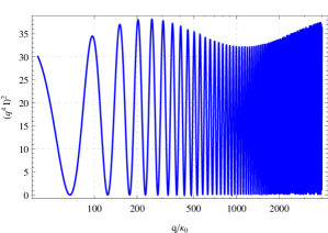
Figure 1: The log periodic oscillation in the $r^{2}$ transition matrix element. Left: near the threshold. Right: at the high frequency tail.

The Quadrupole matrix element — The quadrupole operator $\sum_{j}r_{j}^{2}Y_{2}^{M}(\hat{r}_{j})$ connects the $L=0$ bound state with $L=2$ scattering states. In this case the reduced matrix element takes the form

$$I_{d}(\kappa,q)=\frac{3}{2}\sqrt{5}\int_{0}^{\infty}d\rho\mathcal{R}_{B}^{*}(\rho)\rho^{2}\mathcal{R}_{d}(\rho)\int d\Omega\Phi_{f}^{*}(\Omega)\sum_{j}\cos^{2}\alpha_{j}Y_{20}(\hat{y}_{j})\Phi_{i}(\Omega).$$ (14)

In this case we find no log-periodic oscillations near threshold. Such oscillations, however, modulate the high energy tail of the response function, attenuated by $q^{-4}$ and masked by the linear phase shift variation. These high energy oscillations appear not only in these cases but in all partial waves Bazak and Barnea (2013).

The relative contribution of the $s,d$ modes to the trimer formation is displayed in Fig. 2, where the last term in parenthesis on the rhs of Eq. (4) is presented normalized, along with the $s$ and $d$ components. Similarly to the dimer formation case Bazak et al (2012), the $s$-wave association is peaked around $q=\kappa/2$, while the $d$-wave association is peaked at $q=\kappa$.

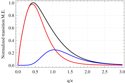
Figure 2: The normalized three-body transition matrix element, Eq. (4), as a function of the relative momentum $q/\kappa$. The sum (black), $r^{2}$ (red, peaked at $q=\kappa/2$), and quadrupole (blue, peaked at $q=\kappa$) terms are given for the unitary point, $|a|=\infty$.

V Conclusion

We have applied the multipole expansion to study trimer photoassociation in ultracold atomic gases. The two dominant modes, at order $k^{5}$, are studied and their relative contribution is shown. Log periodic oscillations are shown in two cases: (i) for the leading s-wave mode, near the threshold, and (ii) for all partial waves at the high frequency tail.