Dirac edges of fractal magnetic minibands in graphene with hexagonal moiré superlattices

Abstract

We find a systematic reappearance of massive Dirac features at the edges of consecutive minibands formed at magnetic fields $B_{p/q}\!=\!\tfrac{p}{q}\phi_{0}/S$ providing rational magnetic flux through a unit cell of the moiré superlattice created by a hexagonal substrate for electrons in graphene. The Dirac-type features in the minibands at $B\!=\!B_{p/q}$ determine a hierarchy of gaps in the surrounding fractal spectrum, and show that these minibands have topological insulator properties. Using the additional $q$-fold degeneracy of magnetic minibands at $B_{p/q}$, we trace the hierarchy of the gaps to their manifestation in the form of incompressible states upon variation of the carrier density and magnetic field.

The fractal spectrum of electron waves in crystals subjected to a strong magnetic field zak_physrev_1964 ; brown_physrev_1964 is a fundamental result in the quantum theory of solids stat_phys_LL . In particular, the bandstructure of electrons on a two-dimensional (2D) lattice is fractured into multiple bands which occur at the values $B_{\frac{p}{q}}=\frac{p}{q}\phi_{0}/S$ of the field providing a rational fraction of magnetic flux quantum $\phi_{0}=h/e$ per unit cell area $S$ zak_physrev_1964 ; stat_phys_LL . Its image hofstadter_prb_1976 , obtained for a square lattice hopping model, known as the Hofstadter butterfly, has stimulated numerous attempts to observe the fractal spectrum of electrons via quantum transport measurements. Since the sparsity of the spectrum increases for larger values of the denominator $q$ in $\tfrac{p}{q}$ (hence smaller gaps), the observation of fractal magnetic bands in real crystals would require unsustainably strong magnetic fields. Hence, early efforts were focused on 2D electrons in periodically patterned GaAs/AlGaAS heterostructures semiconductor_superlattices , where the superimposed superlattice period was made large enough to obtain low denominator fractions within the experimentally available steady magnetic field range. The more recent observation of moiré superlattices, both for twisted bilayer graphene twisted_blg and graphene residing on substrates with hexagonal facets moire_metals , has shown an alternative way to create a long-range periodic potential for electrons: by making lattice-aligned graphene heterostructures using a hexagonal crystal with an almost commensurate period. For this, hexagonal boron nitride (hBN, with the lattice constant of $l_{hBN}=2.50\,\text{\AA}$ vs $l=2.46\,\text{\AA}$ in graphene) provides a perfect match. Several observations of moiré superlattice effects in graphene-hBN heterostructures have already been reported ponomarenko_nature_2013 ; dean_nature_2013 ; hunt_science_2013 .

In this article, we study magnetic minibands caused by a moiré superlattice in graphene. When the surface layer of the substrate is inversion symmetric, the zero-magnetic-field spectra displays clear secondary Dirac points at the first miniband edge wallbank_prb_2013 ; ortix_prb_2012 ; kindermann_prb_2012 . We find that generations of massive Dirac electrons systematically reappear at the edges of magnetic minibands at $B\!=\!B_{\frac{p}{q}}$, and the surrounding fractal spectrum groups around $q$-fold degenerate Landau levels (LLs) of gapped Dirac electrons in an effective magnetic field $\delta\!B\!=\!B-B_{\frac{p}{q}}$. As the Dirac model features a “zero-energy” LL, separated by the largest gap from the rest of the spectrum, this determines a specific hierarchy of gaps in the Hofstadter butterfly, resulting in a peculiar sequence of dominant incompressible states of electrons in graphene-hBN heterostructures in a strong magnetic field.

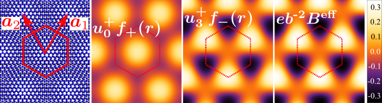
Figure 1: Moiré pattern ($\bm{a}_{1}\!=\!a(\tfrac{1}{2},\tfrac{\sqrt{3}}{2})$, $\bm{a}_{2}\!=\!a(\tfrac{-1}{2},\tfrac{\sqrt{3}}{2})$, unit cell area $S\!=\!\tfrac{\sqrt{3}}{2}a^{2}$) and effective perturbations for electrons in graphene on an hexagonal substrate [$\theta\!=\!0$, and $V^{+}\!=\!0.063vb$, $V^{-}\!=\!0$ in Eqs. (1-2)].

For graphene electrons we use the effective Dirac theory, where the form of moiré perturbation depends on the detailed structure and symmetry of the underlying surface. The phenomenological model for the moiré superlattice wallbank_prb_2013 is given by the Hamiltonian,

$$\!\hat{H}= v\bm{p}\!\cdot\!\bm{\sigma}+vb\!\left(u_{0}^{+}f_{+}\!+\!u_{0}^{-}f_{-}\right)+\xi vb\sigma_{3}\!\left(u_{3}^{+}f_{-}\!+\!u_{3}^{-}f_{+}\right)$$

$$+\xi v\bm{\sigma}\!\cdot\!\left[\bm{l}_{z}\!\times\!\nabla\!\left(u_{1}^{+}f_{-}\!+\!u_{1}^{-}f_{+}\right)\right]\!.$$ (1)

Here $\sigma_{i}$ are Pauli matrices, acting on Bloch states $(\phi_{AK},\phi_{BK})^{T}$ in the $K$ valley ($\xi=1$) and $(\phi_{BK^{\prime}},-\phi_{AK^{\prime}})^{T}$ in the $K^{\prime}$ valley ($\xi=-1$). In the Dirac term, $\bm{p}\!=\!-i\nabla+e\bm{A}$, ($\hbar=1$) describes momentum relative to the valley center, and $[\nabla\times\bm{A}]_{z}=B$. The rest of Eq. (1) describes the superlattice perturbation: a simple potential modulation, a local $A$-$B$ sublattice asymmetry, and the variation of the $A$-$B$ hopping mimicking a pseudo-magnetic field $eB^{\text{eff}}=\xi b^{2}(u_{1}^{+}f_{-}+u_{1}^{-}f_{+})$. Here, $f_{\pm}=\!\sum_{m}\!(\pm 1)^{m+\frac{1}{2}}e^{i\bm{b}_{m}\cdot\bm{r}}$, where the reciprocal lattice vectors, $\bm{b}_{m=0,\cdots,5}$, responsible for the dominant contribution to the superlattice perturbation twisted_blg ; ortix_prb_2012 ; kindermann_prb_2012 ; wallbank_prb_2013 , are related by $60^{\circ}$ rotations (Fig. 2) with $b\equiv|\bm{b}_{m}|\approx\frac{4\pi}{\sqrt{3}l}\sqrt{\delta^{2}+\theta^{2}}$, ($\delta=l_{hBN}/l-1\approx 2\%$ and $\theta\ll 1$ is the misalignment angle).

Six dimensionless parameters $u_{i}^{\pm}$ in Eq. (1) describe the 2D inversion symmetric/asymmetric part of the moiré perturbation. They can take arbitrary values, but two microscopic models, one based on the hopping between the graphene and hBN lattices kindermann_prb_2012 , and the other on scattering of graphene electrons off quadrapole electric moments in the hBN layer wallbank_prb_2013 , predict that

$$vb\{u_{i=0,1,3}^{\pm}\}=V^{\pm}\left\{\frac{\pm 1}{2},\frac{-\delta}{\sqrt{\delta^{2}\!+\!\theta^{2}}},\frac{-\sqrt{3}}{2}\right\}.$$ (2)

We also assume that $|V^{+}|>|V^{-}|$, since only one of the two atoms, B or N, would produce the dominant effect, thus making the moiré perturbation almost inversion-symmetric. In the absence of a magnetic field, the inversion-symmetric perturbation prescribes a gapless miniband spectrum, with a secondary Dirac-point (DP) either at the edge of the first miniband, or embedded into a continuous spectrum at higher energies, whereas the asymmetric part may open gaps both at the zero-energy DP, $\Delta_{0}$, and the secondary DP, $\Delta_{1}$, on the conduction/valence band side ($s=\pm 1$),

$$\Delta_{0}=24vb|u^{+}_{1}u^{-}_{0}+u^{+}_{0}u^{-}_{1}|,$$

$$\Delta_{1}=\sqrt{3}|u^{-}_{0}+2s\xi u^{-}_{1}-\sqrt{3}\zeta u^{-}_{3}|.$$ (3)

To adapt the analysis of the electron spectrum in a magnetic field to the hexagonal symmetry of the moiré pattern, we shall use a non-orthogonal coordinate system, $\bm{r}=x_{1}\frac{\bm{a}_{1}}{a}+x_{2}\frac{\bm{a}_{2}}{a}$, (see Fig. 1), and the Landau gauge, $\bm{A}\!=\!Bx_{1}(-\bm{a}_{1}+2\bm{a}_{2})/(\sqrt{3}a)$. Then, the “free” massive Dirac electrons and the basis of LL states are described by

$$H_{D}=\left(\begin{array}[]{cc}\tfrac{1}{2}\xi\Delta&vd^{\dagger}\\ vd&\tfrac{-1}{2}\xi\Delta\end{array}\right),$$ (6)

$$d=\frac{-2}{\sqrt{3}}\left[\partial_{x_{1}}e^{i\frac{2\pi}{3}}+(\partial_{x_{2}}+i\sqrt{3}eBx_{1}/2)e^{-i\frac{2\pi}{3}}\right]\!,$$

$$\psi_{0}^{k_{2}}\!=\!\frac{e^{ik_{2}x_{2}}}{\sqrt{L}}\!\begin{pmatrix}\frac{1-\beta}{2}\varphi_{0}\\ \frac{1+\beta}{2}\varphi_{0}\end{pmatrix}\!,\quad\psi_{n\neq 0}^{k_{2}}\!=\!\frac{e^{ik_{2}x_{2}}}{\sqrt{2L}}\!\begin{pmatrix}\varphi_{n^{\!-}}\\ c_{n}\varphi_{n^{\!+}}\end{pmatrix}\!,$$

$$\varphi_{n}\!=\!A_{n}e^{-\frac{z^{2}}{2}+\beta\frac{iz^{2}}{2\sqrt{3}}}\mathbb{H}_{n}(\!z\!),\quad z\!=\frac{\sqrt{3}x_{1}}{2\lambda_{B}}+\beta k_{2}\lambda_{B}.$$

Here, $\beta\!=\!B/|B|$, $A_{n}\!=\!\sqrt{3}/(\sqrt{n!2^{(n+1)}\lambda_{B}\sqrt{\pi}})$, $n^{\pm}\!=\!|n|\pm(\beta\mp 1)/2$, $c_{n}\!=\!\beta e^{i\frac{2\pi}{3}}\lambda_{B}(E_{n}-\xi\Delta/2)/(v\sqrt{2|n|})$, $\mathbb{H}_{n}$ is the Hermite polynomial, and $\lambda_{B}\!=\!1/\sqrt{|eB|}$ is the magnetic length. The LL spectrum of the gapped Dirac model is

$$E_{0}=\frac{-\beta\xi\Delta}{2},\qquad E_{n\neq 0}=\text{sign}(n)\sqrt{\frac{\Delta^{2}}{4}+\frac{2|n|v^{2}}{\lambda^{2}_{B}}}.$$ (7)

Figure 2: Example of the moiré superlattice Brillouin zone (larger hexagon, with area $\sqrt{3}b^{2}/2$, and reciprocal lattice vectors $\bm{b}_{m}$), and the two smaller magnetic Brillouin zones (shaded blue, discussed in the text). Red dots show $k_{2}$ values used to construct Bloch states $|_{t,\bm{k}}^{n,j}\rangle$.

For a magnetic field, $B_{\frac{p}{q}}\!=\!\frac{p}{q}\phi_{0}/S$, the electronic spectrum can be described in terms of minibands of Wannier states on a $q$-times larger period superlattice with an integer number of flux quanta per super-cell. For the unit cell enlarged $q$-times zak_physrev_1964 ; stat_phys_LL , e.g., in the $\bm{a}_{1}$ direction, the Brillouin Zone (BZ) is $q$-times smaller than the moiré BZ (Fig. 2), with the dispersion repeated inside it with the period $\bm{b}_{1}/q$. To preserve the point group symmetries, here we enlarge the unit cell $q$-times in all directions, folding the momentum space on to a magnetic BZ with area $\sqrt{3}b^{2}/(2q^{2})$, where each energy band is $q$-fold degenerate brown_physrev_1964 .

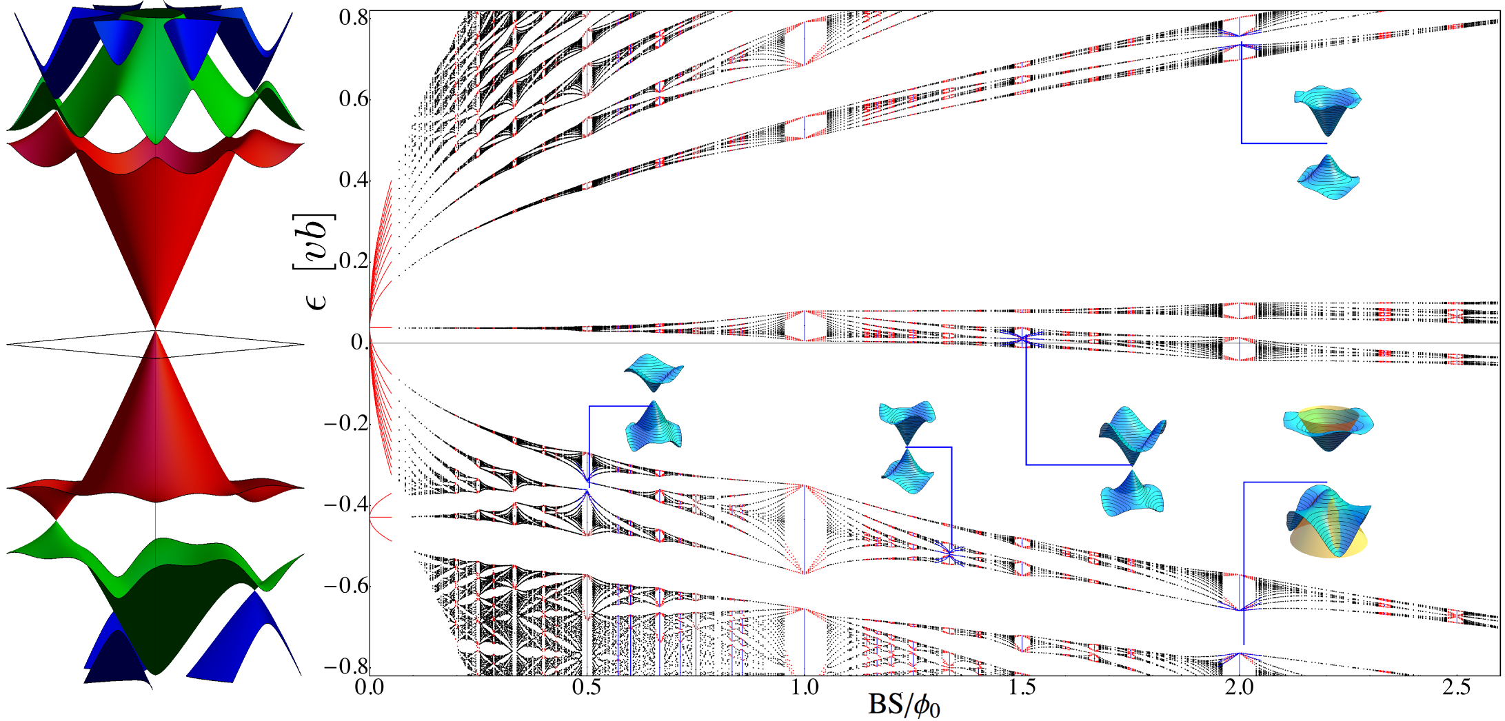
Figure 3: Fractal energy spectrum found by exact numerical diagonalization. The insets show examples of magnetic minibands, at $B_{p/q}\!=\!\tfrac{p}{q}\phi_{0}/S$, and their fit (in yellow) with Dirac spectra used to calculate the energies of effective Dirac Landau levels. The panel on the left shows the $B\!=\!0$ minibands with a distinct secondary Dirac point in the valence band.

The degeneracies of magnetic minibands can be deduced from the properties of the group, $G_{M}=\{\Theta_{\bm{X}}\equiv e^{ieBm_{1}a\frac{\sqrt{3}}{2}x_{2}}T_{\bm{X}},\bm{X}=m_{1}\bm{a}_{1}+m_{2}\bm{a}_{2}\}$, of magnetic translations, where $T_{\bm{X}}$ are the geometrical translations, and

$$\Theta_{\bm{X}}\Theta_{\bm{X}^{\prime}}=e^{i2\pi\frac{p}{q}m_{1}^{\prime}m_{2}}\Theta_{\bm{X}+\bm{X}^{\prime}},$$

$$\Theta_{\bm{X}}\Theta_{\bm{X}^{\prime}}=e^{i2\pi\frac{p}{q}(m_{1}^{\prime}m_{2}-m_{1}m_{2}^{\prime})}\Theta_{\bm{X}^{\prime}}\Theta_{\bm{X}}.$$

The subgroup of $G_{M}$ made of translations $\bm{R}=m_{1}q\bm{a}_{1}+m_{2}q\bm{a}_{2}$ on a $(q\times q)$-enlarged superlattice is isomorphic to the simple group of translations, $T_{\bm{R}}$, so that its eigenstates, $\Theta_{\bm{R}}|_{t,\bm{k}}^{n,j}\rangle=e^{i\bm{k}\cdot\bm{R}}|_{t,\bm{k}}^{n,j}\rangle$, form a plane wave basis. Since the non-abelian group $G_{M}$ has $q$-dimensional irreducible representations brown_physrev_1964 , the spectrum of such plane-wave states is $q$-fold degenerate. Below, we use a basis of Bloch functions built from the LLs in Eq. (6),

$$|_{t,\bm{k}}^{n,j}\rangle=\!\frac{1}{\sqrt{N}}\!\sum_{s}e^{-ik_{1}qas}\psi_{n}^{k_{2}+\frac{\sqrt{3}}{2}b(ps+j+\frac{tp}{q})},\quad j=1,\cdots p$$

where the sum runs over $s=-N/2,\cdots,N/2$, ($N\to\infty$). This basis is similar to the set of Bloch states for a one-dimensional chain with $p$ sites per elementary unit cell, and multiple atomic orbitals on each site labeled by the LL index, $n$. One more index $t\!=\!0,\cdots q\!-\!1$ takes into account the above-mentioned $q$-fold degeneracy, and $\bm{k}\!=\!k_{1}\hat{\bm{k}}_{1}+k_{2}\hat{\bm{k}}_{2}$, $|k_{i}|\!<\!\frac{\sqrt{3}}{4q}b$, $\hat{\bm{k}}_{i}\cdot\frac{\bm{a}_{j}}{a}=\delta_{i,j}$.

Then, we calculate the matrix elements,

$$\langle_{t,\bm{k}}^{n,j}|H|_{\tilde{t},\tilde{\bm{k}}}^{\tilde{n},\tilde{j}}\rangle=\delta_{t,\tilde{t}}\delta_{\bm{k},\tilde{\bm{k}}}\sum_{s}e^{-ik_{1}qas}\mu_{n\tilde{n}}^{k_{2}+\frac{\sqrt{3}}{2}bj,\,k_{2}+\frac{\sqrt{3}}{2}b(ps+\tilde{j})},$$

and find that the index $t$ is conserved, since $[\Theta_{\bm{X}},H]=0$ and $\Theta_{\bm{a}_{1}}|_{t,\bm{k}}^{n,j}\rangle=|_{t+1,\bm{k}}^{n,j}\rangle$, $\Theta_{\bm{a}_{2}}|_{t,\bm{k}}^{n,j}\rangle=e^{i\frac{2\pi pt}{q}}e^{i\bm{k}\cdot\bm{a}_{2}}|_{t,\bm{k}}^{n,j}\rangle$. Also, since Hamiltonian (1) contains only the simplest moiré harmonics, the sum in the above expression is limited to $s\!=\!0,\pm 1$,

$$\mu_{n\tilde{n}}^{k_{2}\tilde{k}_{2}}=\delta_{n,\tilde{n}}\delta_{k_{2},\tilde{k}_{2}}E_{n}+\xi\beta v\sum_{m}(u_{1}^{+}(-1)^{m}-iu_{1}^{-})[e^{i2\pi/3}s_{\tilde{n}}(ib_{m}^{1}+b_{m}^{2})M^{n^{-}\!,\tilde{n}^{+}}_{m}\!+e^{-i2\pi/3}s_{n}(-ib_{m}^{1}+ib_{m}^{2})M^{n^{+}\!,\tilde{n}^{-}}_{m}]$$

$$\qquad\quad\;+vb\sum_{m}(u_{0}^{+}+i(-1)^{m}u_{0}^{-})[M^{n^{-}\!,\tilde{n}^{-}}_{m}\!+s_{n}s_{\tilde{n}}M^{n^{+}\!,\tilde{n}^{+}}_{m}]+\xi vb\sum_{m}(u_{3}^{-}+i(-1)^{m}u_{3}^{+})[M^{n^{-}\!,\tilde{n}^{-}}_{m}\!-s_{n}s_{\tilde{n}}M^{n^{+}\!,\tilde{n}^{+}}_{m}]$$

$$M_{0}^{n_{1}\!,n_{2}}\!\!=\!e^{i\beta\lambda^{2}\!\sqrt{3}}\delta^{-}W_{1,\text{-}1,\text{-}1}^{n_{1}\!,n_{2}},\;M_{1}^{n_{1}\!,n_{2}}\!\!=\!\delta^{-}W_{\text{-}1,1,0}^{n_{1}\!,n_{2}},\;M_{2}^{n_{1}\!,n_{2}}\!\!=\!\delta^{0}W_{\text{-}1,0,1}^{n_{1}\!,n_{2}},\;M_{3}^{n_{1}\!,n_{2}}\!\!=\!e^{i\beta\lambda^{2}\!\sqrt{3}}\delta^{+}W_{\text{-}1,\text{-}1,1}^{n_{1}\!,n_{2}},\;M_{4}^{n_{1}\!,n_{2}}\!\!=\!\delta^{+}W_{1,1,0}^{n_{1}\!,n_{2}},$$

$$M_{5}^{n_{1}\!,n_{2}}\!\!=\!\delta^{0}W_{1,0,\text{-}1}^{n_{1}\!,n_{2}},\quad W_{c_{1},c_{2},c_{3}}^{n_{1},n_{2}}=\frac{N_{n_{1},n_{2}}}{3}\lambda_{B}A_{n_{1}}A_{n_{2}}2^{\bar{n}}\sqrt{\pi}\underline{n}!L_{\underline{n}}^{|\delta\!n|}\!(2\lambda^{2})\,e^{\text{-}\lambda^{2}}\lambda^{|\delta\!n|}e^{i|\delta\!n|(c_{1}\!\frac{\pi}{2}+c_{2}s_{\!\delta\!n}\beta\!\frac{\pi}{3})}e^{i\beta c_{3}\lambda^{2}4k_{2}/b}$$

Here $L_{n}^{\alpha}\!(x)$ is the associated Laguerre polynomial, $\lambda\!=\!b\lambda_{B}/2$, $\delta^{\pm}\!=\!\delta_{\tilde{k}_{2},k_{2}\pm\sqrt{3}b/2}$, $\delta^{0}\!=\!\delta_{\tilde{k}_{2},k_{2}}$, $\bar{n}\!=\!\text{max}[n_{1},n_{2}]$, $\underline{n}\!=\!\text{min}[n_{1},n_{2}]$, $\delta\!n\!=\!n_{1}-n_{2}$, $s_{n}\!=\!\text{sign}(n)$, and $N_{n_{1}\!,n_{2}}\!=\!(1\!-\!\delta_{n_{1}\!,\text{-}1})\!(1\!-\!\delta_{n_{2}\!,\text{-}1})\!\sqrt{1\!+\!\delta_{n_{1}\!,0}}\sqrt{1\!+\!\delta_{n_{2}\!,0}}$.

Figure 3 shows a typical fractal spectrum of magnetic minibands, as a function of the magnetic flux $\phi=SB$ per moiré supercell: this one calculated for the inversion-symmetric superlattice perturbation with $V^{+}\!=\!0.063vb$ and $V^{-}\!=\!0$, $\theta\!=\!0$, by diagonalizing $H$, in the basis $|_{t,\bm{k}}^{n,j}\rangle$ (with a large enough range of $n$ to ensure convergence). The $B\!=\!0$ miniband spectrum is displayed on the left, with the main DP and a secondary DP in the valence band. For $\phi\lesssim 0.2\phi_{0}$, the magnetic miniband spectra can be traced to the analytically calculated sequence of LLs associated with the two DPs.

At a higher flux, the LLs transform into a fractal spectrum with a hierarchy of bands and gaps, which can be understood upon analyzing the dispersion of electrons at the simplest flux fractions $\phi\!=\!\phi_{0}p/q$ (e.g. $\phi\!=\!\tfrac{1}{2}\phi_{0}$, $\tfrac{4}{3}\phi_{0}$, $\tfrac{3}{2}\phi_{0}$) and integer flux (e.g. $\phi\!=\!2\phi_{0}$) shown as insets in Fig. 3. We find that the edges of many of the consecutive bands can be described in terms of a weakly gapped Dirac spectrum, with $\Delta$ and $v_{\text{eff}}$ determined by a fit. Then, the largest gaps in the surrounding fractal spectrum at $B\!=\!B_{p/q}+\delta\!B$ can be interpreted chang_prl_1995 in terms of weakly broadened LLs of these next generation Dirac electrons, evaluated using Eq. (7) and parameters $\Delta$, $v\!\rightarrow\!v_{\text{eff}}$, and $B\!\rightarrow\!\delta\!B$. The analytically calculated effective LLs are shown in blue in the vicinity of the corresponding rational flux values. They interpolate the groups of minibands into the interval where the exact diagonalization becomes impractical, due to the basis set size. This correspondence can be seen best in the cases when the gap $\Delta$ between consecutive minibands is small, and the largest gaps are around the broadened “$n\!=\!0$” LL of the corresponding effective Dirac model. The presence of Dirac-type features indicates that the corresponding 2D system in a magnetic field has the properties of a topological insulator, with chiral edge-states inside the band gaps responsible for the formation of the quantum Hall effect.

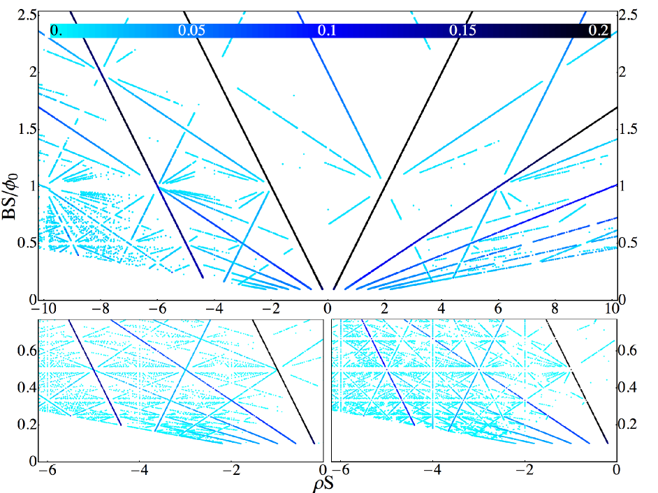
Figure 4: Density-magnetic field diagram showing incompressible electrons states in the fractal spectrum of magnetic minibands. Larger gaps are shown using a darker color. The two panels at the bottom are used to demonstrate the effect of an inversion asymmetric perturbation.

In the upper and lower left panels of Figure 4 we produce a map of incompressible states formed upon filling the minibands in Fig. 3, taking into account that each magnetic miniband at $B_{p/q}$ accommodates a density $\delta\!\rho_{p/q}=g_{s}g_{v}/(qS)$ of electrons, and using darker color to reflect larger gaps in the fractal spectrum. As a reference, we use the largest gaps around the broadened “$n\!=\!0$” LL traced to the main DP in graphene. This is shown as the darkest lines corresponding to filling factors $\nu=\pm 2$. Other dark lines correspond to the large gaps surrounding the “$n\!=\!0$” LLs in the next generation of Dirac electrons, e.g. in the vicinity of $B_{1}$, $B_{1/2}$. They form fan-plots $\rho(B)$ in which the gradient changes at inter-crossings by

$$\delta\!\!\left[\frac{d\!\rho}{d\!B}\right]=\frac{g_{s}g_{v}q}{\phi_{0}}$$

reflecting the additional $q$-fold degeneracy of states in magnetic minibands at $B_{p/q}$ ($g_{s}\!=\!g_{v}\!=\!2$ account for spin-valley degeneracy). For example the darkest lines change the slope by $\delta[d\rho/dB]\!=\!8/\phi_{0}$ when crossing at $B_{1/2}$, in contrast to $\delta[d\rho/dB]\!=\!4/\phi_{0}$ at $B_{1}$.

Having investigated many different realizations of the hexagonal moiré superlattice in Eq. (1), we conclude that robust Dirac-like features in the magnetic miniband spectrum have a systematic appearance. To mention, a Dirac-like band has been found in the Hofstadter spectrum of a tight-binding model on a square lattice with flux $\phi=\tfrac{1}{2}\phi_{0}$ per unit cell hou_pra_2009 ; delplace_prb_2010 . We also analyzed different realizations of hexagonal moiré superlattices described by Eq. 1, and found that the only qualitative difference comes from the inversion symmetry breaking in the unit cell: the interplay between spatial and time inversion asymmetries lifts the valley degeneracy footnote:inv_sym of the fractal spectra. The lower-right panel of Fig. 4 offers an example of the incompressibility map calculated for an inversion-asymmetric perturbation in Eqs. (1-2) with $V^{-}\!=\!0.1V^{+}$. Here the Dirac-like features and the corresponding hierarchy of gaps in the magnetic minibands persist, but the fan diagram acquires additional lines, intercrossing with $\delta[d\!\rho/d\!B]\!=\!g_{v}q/\phi_{0}$.

Acknowledgements. We thank A. Geim, P. Jarillo-Herrero, P. Kim, K. Novoselov and D. Weiss for useful discussions. This work was funded by the EU Flagship Project, EPSRC Science and Innovation Award and Grant EP/L013010/1, and ERC Synergy Grant Hetero2D.