Synchrony and Periodicity in an Excitable Stochastic Neural Network with multiple subpopulations

Abstract

We consider a fully stochastic excitatory neuronal network with a number of subpopulations with different firing rates. We show that as network size goes to infinity, this limits on a deterministic hybrid model whose trajectories are discontinuous. The jumps in the limit correspond to large synchronous events that involve a large proportion of the network. We also perform a rigorous analysis of the limiting deterministic system in certain cases, and show that it displays synchrony and periodicity in a large region of parameter space.

1 Introduction

The study of oscillator synchronization has made a significant contribution to the understanding of the dynamics of real biological systems [5, 29, 28, 32, 19, 18, 8, 39, 12, 22, 40, 7, 20, 31], and has also inspired many ideas in modern dynamical systems theory. See  [36, 33, 43] for reviews.

The prototypical model in mathematical neuroscience is a system of “pulse-coupled” oscillators, that is, oscillators that couple only when one of them “fires”. More concretely, each oscillator has a prescribed region of its phase space where it is active, and only then does it interact with its neighbors. There has been a large body of work on deterministic pulse-coupled networks [24, 13, 38, 41, 4, 37, 42, 6, 23, 32, 29, 34], mostly studying the phenomenon of synchronization on such networks.

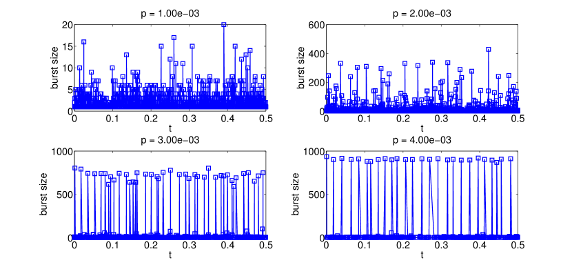
In [9, 10], the first author and collaborators considered a specific example of a network containing both refractoriness and noise; the particular model was chosen to study the effect of synaptic failure on the dynamics of a neuronal network. What was observed in this class of models is that when the probability of synaptic success was taken small, the network looked, more or less, like a stationary process, with a low degree of correlation in time; when the probability of synaptic success was taken large, the system exhibited synchronous behavior that was close to periodic. Both of these behaviors are, of course, expected: strong coupling tends to lead to synchrony, and weak coupling tends not to. The most interesting observation was that for intermediate values of the coupling, the network could support both synchronized and desynchronized behaviors, and would dynamically switch between the two.

The main mathematical results of [10] explained this phenomenon in two ways: it first showed that in the limit $N\to\infty$, the dynamics of the neuronal network limited onto a deterministic dynamical system. (What was unusual for this model was that the deterministic system was a hybrid system: a system of an continuous flow coupled to a map of the phase space. The effect of this system is to have continuous trajectories which jump at prescribed times.) The second part of the result was to study the dynamics of this hybrid system, and show that in certain parameter regimes the deterministic system was multistable, i.e. had multiple attractors for the dynamics. Putting these two together explained the switching behavior observed in the finite $N$ model, since the stochastic system would switch, on long times scales, between the attractors that exist in the $N\to\infty$ limit.

In this paper, we consider an extension of the model where we allow for several independent subpopulations with different intrinsic firing rates.

Fig. 1: Different behaviors of the model. We fix $M=10$, $N=1000$, and plot different dynamics of the model that correspond to different $p$. As we increase $p$, we see the change from asynchronous and irregular behavior to synchronous and periodic behavior.

2 Stochastic Model

Our model is a stochastic neuronal network model with all-to-all excitatory coupling whose details we elucidate in this section. We first describe the dynamics of a finite network, then describe the “mean field” limit of the network as we take the network size to infinity.

Fig. 2: The meaning of the blue data: we fix a choice of $\boldsymbol{\alpha}$, $K=2$, and $N=1000$, run the stochastic neuronal network studied in this paper, and plot the burst sizes in light blue. For $p$ large enough, we also plot the mean and standard deviations of the burst sizes for all of the bursts larger than one-tenth the size of the network. In red, we plot the deterministic burst size (as a proportion of network size) in the deterministic limit defined in Section 3.2 below — the main result of Section 3.2 is that the stochastic (blue) system limits to the deterministic (red) system as $N\to\infty$.

2.1 Fixed network size $N$

The state of a single neuron is given by its voltage. We assume here and throughout that the voltage can only take one of a finite number of levels (see [9] for a justification of this, but, in short, it is a reasonable modeling assumption if we assume that the neurons’ leak is sufficiently small). We denote these levels by $\mathcal{K}=\{0,1,\dots,K-1\}$, and throughout $K$ will be the number of voltage levels possible for each neuron. We will assume that the network has $N$ neurons, and thus the entire state space of the network can be represented by $V_{t}=\{V_{n,t}\}_{n=1}^{N}\in\mathcal{K}^{N}$.

If a neuron is ever promoted to level $K$ it is said to “fire”. The effect of neuron $i$ firing is that it potentially raises the level of every other neuron in the network; more precisely, when neuron $i$ fires it promotes neuron $j$ one level with probability $p_{ij}$, if $j$ has not already fired. It is clear that any one neuron firing can lead to multiple other neurons firing, so that there can be a “cascade” of neuronal firings all initiated by the firing of a single neuron. These bursting dynamics are exactly the same as in [10], and we describe these now.

2.1.1 Bursting dynamics

We now give a precise description of a burst, which we will denote by the random partial function $B\colon\mathcal{K}^{n}\to\mathcal{K}^{n}$.

We add two “virtual states” to $\mathcal{K}$, denoted by $Q,P$, where $Q,P$ can be thought of as a “queue” and as “processed” neurons, respectively. Then, let us assume that there exists a $t>0$ such that $V_{i,t}=K$ for a single $i$. Define the initial sets as:

$$S_{k,0}=\{j:V_{j,t}=k\},\quad Q_{0}=\{i\},\quad P_{0}=\{\}.$$

For $i,j\in[N]$ and $u\in\mathbb{N}$, define the Bernoulli random variables $\eta_{i,j}^{(u)}$ where $\mathbb{P}(\eta_{i,j}^{(u)}=1)=p_{ij}$, independently. For each $n$, define

$$\zeta_{j}^{(u)}=\sum_{i\in Q_{n}}\eta_{ij}^{(u)},$$

which represents the number of kicks that neuron $j$ receives from neurons currently in the queue. We then define

$$S_{k,u+1} =\bigcup_{\ell=0}^{k}\{j:j\in S_{k-\ell,u}\wedge\zeta_{j}^{(u)}=\ell\},\quad Q_{u+1}=\bigcup_{\ell=0}^{N}\{j:j\in S_{K-\ell,u}\wedge\zeta_{j}^{(u)}\geq\ell\},$$

$$P_{u+1} =Q_{n}.$$

In words, we promote every neuron up $\zeta_{j}^{(u)}$ steps, unless this number is large enough to bring the neuron to level $K$ or above. If this happens, we put the neuron in the queue, and we move every neuron currently in $Q$ to $P$.

It is clear from this definition that if $Q_{u}=\emptyset$, then the process stops evolving, since $\zeta_{j}^{(u)}=0$ for all $j$. Define $u^{*}=\inf_{u>0}Q_{u}=\emptyset$ and only evolve the process for $u=1,\dots,u^{*}$. We then define

$$S_{0,u^{*}+1}=S_{0,u^{*}}+P_{u^{*}},\quad S_{k,u^{*}+1}=S_{k,u^{*}},k>0,$$

i.e. at the end of the burst, we place all of the processed neurons back at level 0. We then define the map $B(V_{t})=\{B_{i}(V_{t})\}_{i=1}^{N}$ by

$$B_{i}(V_{t})=k\Leftrightarrow i\in S_{k,u^{*}+1}.$$

This is the definition if a single component of $V_{t}$ is at level $K$. If all of the components of $V_{t}$ are $\leq k$, then we define $B(\cdot)$ to be the identity. If more than one component of $V_{t}$ is at level $K$, we say that $B$ is undefined. (Of course, it is clear how we should define $B(\cdot)$ on this set, but we will see below that this state can never occur in our dynamics, so we say that $B$ is undefined on this state to stress this.)

2.1.2 Non-bursting dynamics

Here we specify what happens to the network between the bursts. This is where we differ from the model of [9, 10].

Choose $\boldsymbol{\rho}=\{\rho_{n}\}_{n=1}^{N}$, with $\rho_{n}>0$, and we assume that neuron $n$ is stimulated by a exogeneous forcing of rate $\rho_{n}$. More precisely, given the state $V_{t}$, choose $n$ independent exponential random variables $T_{n}$, define $U_{n}=T_{n}/\rho_{n}$, and let $n^{*}=\inf_{n\in[N]}U_{n}$. We then say that $V_{t}$ is defined to be constant on $[t,t+U_{n})$, and

$$V_{t+U_{n^{*}}}=B(V_{t}+\widehat{e}_{n^{*}}),$$

where $\widehat{e}_{k}$ is the vector with a one in the $k$th slot and zero elsewhere.

In words, what we do is promote the level of $V_{n^{*},t}$ by one level and leave all the other neurons alone. Recall that by the definition of $B(\cdot)$ above, if the neuron that we have just promoted did not reach level $K$, then we do nothing else. If it did, then we compute the random map $B(\cdot)$ as described above.

From this and some elementary results for Markov chains [30], we see that this defines a continuous-time Markov chain for all $t>0$, once we have specified $V_{0}$. It follows from the various theorems of [30] that $n^{*}$ is unique, and $U_{n^{*}}<\infty$ with probability one. Moreover, by construction, $V_{t}$ is a cádlág process, i.e. a stochastic process that is right-continuous with countably many discontinuities.

Many readers might be familiar more with an alternative description of the process above, where we could have said that, given the state $V_{t}$ and $\Delta t\ll 1$, the probability of any neuron being promoted is $\Delta t\cdot\sum_{n=1}^{N}\rho_{n}$, and, given that a neuron is promoted, the probability that it is neuron $i$ is given by $\rho_{i}/\sum_{n=1}^{N}\rho_{n}$, and these two are independent. (This is the formulation of the process sometimes called the “Gillespie method” or the “SSA method” [15, 16, 14, 17] and it is well-known that this definition gives rise to the same stochastic process once it is made sufficiently precise.)

2.2 Mean-field ($N\to\infty$) limit

The stochastic process defined above is perfectly well-defined, but of course for finite $N$, and for various heterogeneous choices of $p_{ij},\rho_{j}$, the dynamics of this system can be quite complicated. As is common in general in the theory of dynamical systems on networks [21, 1, 2, 11], we seek to consider the limit as $N\to\infty$ and hope that a simpler “network level” description can be made.

To make the limit well-defined, we need some sort of assumptions regarding the sets $\{p_{ij}\}_{i,j=1}^{N}$ and $\{\rho_{n}\}_{n=1}^{N}$. In [9, 10], this model was considered under the assumption that $p_{ij}=p$ and $\rho_{n}=\rho$, i.e. the most homogeneous possible example was considered. It was further assumed that $p$ satisfied the scaling law $pN\to\beta$, where $\beta>0$ is fixed.

In this paper, we will consider the following generalization: For each $N$, we define a partition of $N$ into $M$ disjoint sets, denoted by $\{A_{m}^{(N)}\}_{m=1}^{M}$, and we assume that $\rho$ is constant on each of these subsets. We will abuse notation slightly and denote the rate on subset $A_{m}^{(n)}$ as $\rho_{m}$. We will then consider the limit where $N\to\infty$ where we assume that each subpopulation scales proportionally in the limit, i.e. we choose $\boldsymbol{\alpha}=\{\alpha_{m}\}_{m=1}^{M}$, and $\boldsymbol{\rho}=\{\rho_{m}\}_{m=1}^{M}$, with

(2.1) $$0<\alpha_{m}<1,\quad\sum_{m=1}^{M}\alpha_{m}=1,\quad\rho_{m}>0,$$

and we assume that $||A_{m}^{(N)}|-\alpha_{m}N|<1$ for all $m$. (Note that $\alpha_{m}N$ is not in general an integer, but we assume that $|A_{m}^{(N)}|$ is as close to this number as possible.)

We will then take the limit as $N\to\infty$, $pN\to\beta>0$, and $A_{m}^{(N)}$ scaling as described above. The case where $M=1$ is when all neurons have the same rate, and is thus equivalent to the model studied in [10].

2.2.1 Definition of mean-field limit

The convention that we will use below is as follows: we will always use capital roman letters for stochastic processes, and small Greek letters for deterministic processes. Moreover, superscripts will always correspond to parameters and subscripts with always correspond to coordinates (or time in the case of as stochastic process).

To define the mean-field limit, let us consider the stochastic process defined above with fixed $N,K,p,\boldsymbol{\alpha},\boldsymbol{\rho}$, and let us define the auxiliary process $X$ defined by

$$X^{(N,K,p,\boldsymbol{\alpha},\boldsymbol{\rho})}_{k,m,t}=\#\{n:V_{n,t}=k\ \&\ n\in A_{m}^{(N)}\},$$

i.e. $X_{k,m,t}$ counts the number of neurons at level $k$ in the set $A_{m}^{(N)}$. It is not difficult to see that all of the information needed to evolve the process is contained in the $X$’s. Notice that $X_{k,m,t}\in\mathbb{Z}^{KM}$ for each $t$, and we index it by $(k,m)$.

We now define a deterministic hybrid dynamical system. What makes this system a hybrid system is that there will be two evolutionary rules for the process defined on two different parts of the phase space.

Definition 1.

Let $\boldsymbol{\alpha}$ satisfy 2.1. We define

$$D^{K,{\boldsymbol{\alpha}}}:=\left\{x=\{x_{k,m}\}_{k,m}\in\mathbb{R}^{KM}:\sum_{k=0}^{K-1}x_{k,m}=\alpha_{m}\right\},$$

and write $D^{K,{\boldsymbol{\alpha}}}$ as the disjoint union $D^{K,{\boldsymbol{\alpha}}}=D_{\mathcal{L}}^{K,{\boldsymbol{\alpha}},{\beta}}\dot{\cup}D_{G}^{K,{\boldsymbol{\alpha}},{\beta}}$, where

$$D_{G}^{K,{\boldsymbol{\alpha}},{\beta}}:=\left\{x\in D^{K,{\boldsymbol{\alpha}}}:\sum_{m=1}^{M}x_{K-1,m}\geq\frac{1}{\beta}\right\},\quad D_{\mathcal{L}}^{K,{\boldsymbol{\alpha}},{\beta}}=D^{K,{\boldsymbol{\alpha}}}\setminus D_{G}^{K,{\boldsymbol{\alpha}},{\beta}}.$$

We will also write $\partial D_{G}^{K,{\boldsymbol{\alpha}},{\beta}}$ for the set of $x$ with $\sum_{m=1}^{M}x_{K-1,m}=\beta^{-1}$.

Definition 2.

We now define a deterministic hybrid dynamical system $\xi^{K,{\boldsymbol{\alpha}},{\boldsymbol{\rho}},{\beta}}(t)$ with state space $D^{K,{\boldsymbol{\alpha}}}$. The system will be hybrid since it will have two different rules on two different parts of the phase space.

$\bullet$ if $\xi\in D_{\mathcal{L}}^{K,{\boldsymbol{\alpha}},{\beta}}$, i.e. $\sum_{m=1}^{M}\xi_{K-1,m}(t)<\beta^{-1}$, then we flow by

(2.2) $$\frac{d}{dt}\xi_{k,m}(t)=\rho_{m}\mu(\xi)(\xi_{k-1,m}(t)-\xi_{k,m}(t)),$$

where $\mu(\xi)$ is a scalar function that we define below and we interpret the index modulo $K$; more specifically, if we define the matrix $\mathcal{L}$ by

(2.3) $$\mathcal{L}_{(k,m),(k^{\prime},m^{\prime})}=\begin{cases}-\rho_{m},&k=k^{\prime},m=m^{\prime},\\ \rho_{m},&k^{\prime}=k+1\pmod{K},m^{\prime}=m,\\ 0,&\mbox{otherwise.}\end{cases}$$

then on $D_{\mathcal{L}}^{K,{\boldsymbol{\alpha}},{\beta}}$ we flow according to $\dot{\xi}=\mu(\xi)\mathcal{L}x$. Notice that since $\mu(\xi)$ is scalar, the trajectories of the flow coincide with the trajectories of the flow $\dot{\xi}=\mathcal{L}\xi$ and differ only up to a time change. (Ergo, if we are interested in the trajectories of the system we can ignore $\mu(\xi)$ altogether.)

$\bullet$ We now define a map $G^{K,{\boldsymbol{\alpha}},{\beta}}$ with domain $D_{G}^{K,{\boldsymbol{\alpha}},{\beta}}$. We first define

$$\psi^{K,{\beta}}(\xi,s):=-s+\sum_{i=1}^{K}\sum_{m=1}^{M}\xi_{K-i,m}\left(1-\sum_{j=0}^{i-1}\frac{s^{j}\beta^{j}}{j!}e^{-s\beta}\right)$$

and

$$s_{\star}^{K,{\beta}}(\xi)=\inf_{s>0}\{s\colon\psi^{{K}}\beta(\xi,s)=0\}.$$

Let us now index $\mathbb{R}^{MK+1}$ by $(k,m)$ with $k\in\mathcal{K}$ and $m\in[M]$, plus the state $Q$, and we define the matrix $\mathcal{M}$ whose components are given by

$$\mathcal{M}_{z,z^{\prime}}=\begin{cases}-1,&z=(k,m),z^{\prime}=(k^{\prime},m^{\prime}),k=k^{\prime},m=m^{\prime},\\ 1,&z=(k,m),z^{\prime}=(k^{\prime},m^{\prime}),k^{\prime}=k+1,m^{\prime}=m,\\ 1,&z=(K-1,m),z^{\prime}=Q\\ 0,&\mbox{else}.\end{cases}$$

We then define $G^{K,{\boldsymbol{\alpha}},{\beta}}$ componentwise by

(2.4) $$\begin{split}G^{K,{\boldsymbol{\alpha}},{\beta}}_{{k},{m}}(\xi)&=(e^{\beta s^{*}\mathcal{M}}\xi)_{k,m},\quad k=1,2,\dots,K-1,\\ G^{K,{\boldsymbol{\alpha}},{\beta}}_{{0},{m}}(\xi)&=\alpha_{m}-\sum_{k=1}^{K}(e^{\beta s^{*}\mathcal{M}}\xi)_{k,m}.\end{split}$$

(The final condition guarantees that $G^{K,{\boldsymbol{\alpha}},{\beta}}(\xi)\in D^{K,{\boldsymbol{\alpha}}}$. The interpretation of this is that we redistribute all of the neurons that have fired back to level 0, and we do so in such a way to conserve the total number of neurons in each subpopulation.)

$\bullet$ Finally we combine these to define the hybrid system for all $t>0$. Fix $K,\boldsymbol{\alpha},\boldsymbol{\rho},\beta$. Assume $\xi(0)\in D_{\mathcal{L}}$, and define

(2.5) $$\tau_{1}=\inf_{t>0}\{e^{t\mathcal{L}}\xi(0)\in D_{G}\}.$$

We then define

$$\xi(t)=e^{t\mathcal{L}}\xi(0)\mbox{ for }t\in[0,\tau_{1}),\quad\xi(\tau_{1})=G(e^{\tau_{1}\mathcal{L}}\xi(0)).$$

(Of course, it is possible that $\tau_{1}=\infty$, in which case we have defined the system for all positive time, otherwise we proceed recursively.) Now, given $\tau_{n}<\infty$ and $\xi(\tau_{n})\in D_{\mathcal{L}}$, define

(2.6) $$\tau_{n+1}=\inf_{t>\tau_{n}}\{e^{(t-\tau_{n})\mathcal{L}}\xi(\tau_{n})\in D_{G}\},$$

and

$$\xi(t)=e^{(t-\tau_{n})\mathcal{L}}\xi(\tau_{n})\mbox{ for }t\in[\tau_{n},\tau_{n+1}),\quad\xi(\tau_{n+1})=G(e^{(\tau_{n+1}-\tau_{n})\mathcal{L}}\xi(\tau_{n})).$$

If $\tau_{n}=\infty$ then we define $\tau_{n+1}=\infty$ as well. We call the times $\tau_{1},\tau_{2},\dots$ the big burst times, and we call $s_{\star}^{K,{\beta}}(\xi(\tau_{n}))$ the size of the big burst.

Remark 3.

We note that the definition given above is well-defined and gives a unique trajectory for $t\in[0,\infty)$ if and only if we know that $G(\xi)\in D_{\mathcal{L}}$ for any $\xi\in D_{G}$. We will show below that this is the case. We will also see below that some trajectories have infinitely many big bursts, and some have finitely many—this depends both on parameters and initial conditions.

2.2.2 Intuition behind definition

This is no doubt a complicated description, but all of the pieces of this definition can be well-motivated. The way to think of this model is it is either “subcritical” or “supercritical”: when the model is subcritical, we move according to the flow $e^{t\mathcal{L}}$, and when it is supercritical, we apply the map $G(\cdot)$. The third part of the definition is the way the two pieces are stitched together, and looks a bit complex, but basically boils down to “flow until the trajectory hits a distinguished set; when it does, apply the map $G(\cdot)$, and if it never does, just flow forever”.

The criticality parameter is the sum $\sum_{m=1}^{M}x_{K-1,m}$, which is the number of neurons at level $K-1$ across all subpopulations. The criticality threshold is $\beta^{-1}$. To see why this should be so, we can think of a branching process description of the growth of the queue. Note that all neurons act the same (the only difference between different subpopulations is the rate $\rho_{m}$, which only affect interburst dynamics). Also note that every time we process a neuron in the firing queue, it will promote, on average $px_{K-1,m}N$ neurons from state $x_{K-1,m}$ up to firing. In this scaling, this is $\beta x_{K-1,m}$, and thus the mean number of children that each firing event creates is $\beta\sum_{m=1}^{M}x_{K-1,m}$. Thus the critical threshold is whether this number is less than, or greater than, unity.

When the system is subcritical, whenever a neuron fires, the size of the burst that it generates will be $O(1)$. In the scaling where all events are $O(1)$ inside of a $O(N)$ network, the Markov chain will be well-approximated by the mean-field differential equation [25, 35], and this is exactly the ODE given in the first part above. If we assume that $\mu(x)$ is the mean size of a burst in this regime (again recalling that it is $O(1)$), then it is plausible that we should imagine a “flux” ODE where the rate at which neurons leave a state is proportional to the number in the state, and the rate at which they enter a state is proportional to the size of the bin corresponding to neurons with voltage one level down, and this is (2.2).

When the system is supercritical, there is a positive probability of a burst taking up $O(N)$ neurons, or, an $O(1)$ proportion of the entire network. The description above is meant to capture the size of this burst, $s_{\star}^{K,{\beta}}N$, and its effect. To understand this description, let us consider the case where we have processed $sN$ neurons, i.e. each neuron in the network has been given $sN$ possibilities to be promoted, each with probability $p$. Thus, each neuron in the network will have receive a number of kicks given by the binomial random variable with $sN$ trials each of which with $\beta/N$ probability of success, and it is well known that in the limit as $N\to\infty$, this binomial converges to $Po(s\beta)$, a Poisson random variable with mean $s\beta$. If we rewrite the definition of $\psi^{K,{\beta}}$ in this light, we have

$$\psi^{K,{\beta}}(x,s):=-s+\sum_{i=1}^{K}\sum_{m=1}^{M}x_{K-i,m}\mathbb{P}(Po(s\beta)\geq i),$$

so we see that $\psi^{K,{\beta}}(t)$ is the expected proportion of neurons in the queue at the time when $sN$ neurons have been processed, and thus $s_{\star}^{K,{\beta}}$ is the first time that this is zero. Of course, this is only an expectation, but in fact one can show that this (random) $s_{\star}^{K,{\beta}}$ satisfies a large deviation principle and $o(1)$ far away from its mean in this scaling. Moreover, the map $G$ is the expected value of the system after a burst of size $s_{\star}^{K,{\beta}}$; to see this, notice that the components of $\beta\mathcal{M}$ describes the average effect of processing one neuron from the queue.

Said another way, consider the matrix exponential $e^{\beta s\mathcal{M}}$ in the definition. This is, of course, the solution of the differential equation $d\xi/ds=\beta\mathcal{M}\xi$. One can compute explicitly that, given an initial condition $\xi(0)$, the solution of this ODE satisfies

$$\xi_{k,m}(s)=e^{-s\beta}\sum_{j=0}^{k}\frac{s^{j}\beta^{j}}{j!}\xi_{k-j,m}(0),$$

and similarly that

$$\xi_{Q}(s)=\sum_{i=1}^{k}\sum_{m=1}^{M}\xi_{K-i,m}\left(1-\sum_{j=0}^{i-1}\frac{s^{j}\beta^{j}}{j!}e^{-s\beta}\right)=\psi_{\beta,K}(\xi(0),s)+s.$$

Another interpretation of this definition is that we consider the flow where mass is moving from $\xi_{k,m}$ to $\xi_{k+1,m}$ with rate $\beta$, for all $k=0,1,\dots,K-2$, and the mass from each $\xi_{K-1,m}$ is moving to $Q$ with rate $\beta$ as well. If we then assume that mass is leaving $Q$ at rate $1$, then $\psi^{K,{\beta}}(s)$ is exactly the size of $Q$, and thus $s_{\star}^{K,{\beta}}$ is the time $s$ at which $\xi_{Q}(s)=s$ under the $\mathcal{M}$ flow; said another way, if the mass is leaking out of the queue at rate one, then this would be the time when the queue is first zero.

From this argument, it is not hard to see that if $x\in D_{G}^{{\boldsymbol{\alpha}},{\beta}}$, then $G(x)\in D_{\mathcal{L}}^{{\boldsymbol{\alpha}},{\beta}}$. To see this, note that since $\xi_{Q}(s)>s$ for some $s>0$, at the first time when $\xi_{Q}(s)=s$, we must have

$$1>\frac{d}{ds}\xi_{Q}(s)=\beta\sum_{m=1}^{M}z_{K-1,m}.$$

It is worth noting that the mean-field system is discontinuous whenever the map $G_{\beta}$ is applied and continuous otherwise. Since this discontinuity refers to the instantaneous change in the network when a very large event effects a significant proportion of the network, we will also call these discontinuities “big bursts”. We will see below that there are some initial conditions that lead to infinitely many big bursts, and others that lead to only finitely many.

This process is a generalization of, and quite similar to, the more homogeneous process considered in [10]; readers more interested in the intuition behind this mean-field definition can read Section 3 of that paper.

2.2.3 Convergence Theorem for mean field limit

In this section, we give a precise statement of the convergence theorem of the stochastic neuronal network to the mean-field limit. In the interests of space, we do not give a full proof of the theorem here, but refer the reader to [10]; it is not difficult to see that the same proof as given there will follow with minimal technical changes.

Theorem 4.

Consider any $x\in D_{K,\boldsymbol{\alpha}}\cap\mathbb{Q}^{KM}$. For $N$ sufficiently large, $Nx$ has integral components and we can define the neuronal network process $X^{N,K,\boldsymbol{\alpha},\boldsymbol{\rho},p}_{t}$ as above, with initial condition $X_{0}^{N,K,\boldsymbol{\alpha},\boldsymbol{\rho},p}=Nx$.

Choose and fix $\epsilon,h,T>0$. Let $\xi^{K,{\boldsymbol{\alpha}},{\boldsymbol{\rho}},{\beta}}(t)$ be the solution to the mean-field defined in Definition 2 with initial condition $\xi^{K,{\boldsymbol{\alpha}},{\boldsymbol{\rho}},{\beta}}(0)=Nx$. Define the times $\tau_{1},\tau_{2},\dots$ at which the mean field is discontinuous, and define $b_{min}(T)=\min\{s_{\star}^{K,{\beta}}(\xi(\tau_{k})):\tau_{k}<T\}$, i.e. $b_{min}$ is the size of the smallest big burst which occurs before time $T$, and let $m(T)=\arg\max_{k}\tau_{k}<T$, i.e. $m(T)$ is the number of big bursts in $[0,T]$.

Pick any $\gamma<b_{min}(T)$. For the stochastic process $X^{N,K,\boldsymbol{\alpha},\boldsymbol{\rho},p}_{t}$ and denote by $T^{(N)}_{k}$ the (random) times at which the $X^{N,K,\boldsymbol{\alpha},\boldsymbol{\rho},p}_{t}$ has a burst of size larger than $\gamma N$. Then there exists $C_{0,1}(\epsilon)\in[0,\infty)$ and $\omega(K,M)\geq 1/(M(K+3))$ such that for $N$ sufficiently large,

(2.7) $$\mathbb{P}\left(\sup_{j=1}^{m(T)}\left|{T^{(N)}_{j}-\tau_{j}}\right|>\epsilon\right)\leq C_{0}(\epsilon)Ne^{-C_{1}(\epsilon)N^{\omega(K,M)}}.$$

Moreover, if we define $\mathcal{T}:=([0,T]\setminus\cup_{j=1}^{m(T)}(T_{j}^{(N)}-\epsilon,T_{j}^{(N)}+\epsilon))$, and

$$\varphi(t)=t-(T_{j}^{(N)}-\tau_{j})\mbox{ where }j=\max\{k\colon\tau_{k}<t\},$$

then

(2.8) $$\mathbb{P}\left(\sup_{t\in\mathcal{T}}\left|{N^{-1}X^{N,K,\boldsymbol{\alpha},\boldsymbol{\rho},p}_{t}-\xi^{K,{\boldsymbol{\alpha}},{\boldsymbol{\rho}},{\beta}}(\varphi(t))}\right|>\epsilon\right)\leq C_{0}(\epsilon)Ne^{-C_{1}(\epsilon)N^{\omega(K,M)}}.$$

In summary, the theorem has two main conclusions about what happens if we consider a stochastic neuronal network with $N\gg 1$ and if we consider the corresponding deterministic mean-field system: first, the times of the “big bursts” do in fact line up, and, second, as long as we are willing to excise a small amount of time around these big bursts, the convergence of the stochastic process to the deterministic process is uniform up to a rescaling in time. In short, it is sufficient to consider the deterministic system when the network has a sufficient number of neurons.

The guaranteed rate of convergence is subexponential due to the presence of the $\omega(K,M)$ power in the exponent, but note that the convergence is asymptotically faster than any polynomial. Numerical simulations done for the case of $M=1$ were reported in [9] show that $\omega(K,1)$ seemed to be close to 1, and in fact did not seem to decay as $K$ was increased, suggesting that the lower bound is pessimistic and that the convergence may in fact be exponential. However, the lower bound given in the theorem above seems to be the best that can be achieved by the authors’ method of proof. For the details comprising a complete proof of Theorem 4, see [10].

3 Properties of Mean Field Model for $K=2$

A portion of the results of [10] were an analysis of the deterministic hybrid system $\xi^{K,{\boldsymbol{\alpha}},{\boldsymbol{\rho}},{\beta}}(t)$ when $M=1$. It was shown there that one could compute the solution of the system analytically for $K=2,\beta>0$, but an analytic solution seemed intractable for $K\geq 3$. We want to extend the analysis done there for the $K=2$ case, but for $M>1$.

One of the main results of the deterministic analysis was that the hybrid system was multistable for $K$ sufficiently large: more specifically, it was shown that for all $\beta<K$, there was an attracting fixed point in the model, and for all $\beta>\theta(K)$, there was an attracting periodic orbit, and finally that for some $\gamma\in(0,1)$, $\theta(K)<\gamma K$ for $K$ sufficiently large. Thus there was a parameter regime with multiple stable solutions, which meant that the stochastic system would switch between these attractors on long timescales. The analysis performed in [10] was not able to produce a closed-form solution but used asymptotic matching techniques.

It should be noted that the analysis of this hybrid system is quite difficult. As is well known, the analysis of hybrid systems can be exceedingly complicated [3, 27]; questions just about the stability of fixed points is much more complicated than in the non-hybrid (flow or map) case, and stability of periodic orbits are more complicated still. As we see below, the state of the art technique for this kind of problem is very problem-specific.

3.1 Main result

Note: here and in the following, we will only be considering the case of $K=2$, so that we will drop the $K$ from the notation.

Theorem 5.

Choose $\boldsymbol{\alpha},\boldsymbol{\rho}$ as in (2.1), and recall the definition of the hybrid system $\xi^{{\boldsymbol{\alpha}},{\boldsymbol{\rho}},{\beta}}(t)$ given in Definition 2. For $K=2$, and any $M\geq 1$, there exists $\beta_{M}>0$ such that, for $\beta>\beta_{M}$, the hybrid system has a globally attracting limit cycle $\xi_{\star}^{{\boldsymbol{\alpha}},{\boldsymbol{\rho}},{\beta}}(t)$. This orbit $\xi_{\star}^{{\boldsymbol{\alpha}},{\boldsymbol{\rho}},{\beta}}(t)$ undergoes infinitely many big bursts. Moreover, $\limsup_{M\to\infty}\beta_{M}/\log(\sqrt{M})\leq 1$.

We delay the formal proof of the main theorem until after we have stated and proved all of the auxiliary results below, but we give a sketch here.

The main analytic technique we use is a contraction mapping theorem, and we prove this in two parts. We first show that for any two initial conditions, the flow part of the system stretches the distance between them by no more than $1+\sqrt{M}/2$ (Theorem 11). We then show that the map $G_{\beta}$ is a contraction, and, moreover, its modulus of contraction can be made as small as desired by choosing $\beta$ large enough (Theorem 14). The stretching modulus of one “flow, map” step of the hybrid system is the product of these two numbers, and as long as this is less than one we have a contraction. Finally, we also show that for $\beta>2$, there exists an orbit with infinitely many big bursts (Lemma 7)—in fact, we show the stronger result that all initial conditions give an orbit with infinitely many big bursts. All of this together, plus compactness of the phase space, implies that this orbit is globally attracting.

We would like to point out that several of the steps mentioned above seem straightforward at first glance, but are actually nontrivial for a few reasons.

First, consider the task of computing the growth rate for the flow part of the hybrid system. Clearly $e^{t\mathcal{L}}\cdot$ is a linear contraction, since its eigenvalues are

$$\{0^{M},-2\rho_{1},-2\rho_{2},\dots,-2\rho_{M}\},$$

and the point in the nullspace is unique once $\boldsymbol{\alpha}$ is chosen. However, even though the linear flow $e^{t\mathcal{L}}$ is contracting, and clearly $\left|{e^{t\mathcal{L}}x-e^{t\mathcal{L}}x^{\prime}}\right|<\left|{x-x^{\prime}}\right|$ for any fixed $t>0$, the difficulty is that two different initial conditions can flow for a different interval of time until the first big burst, and clearly we cannot guarantee that $e^{t\mathcal{L}}x$ and $e^{t^{\prime}\mathcal{L}}x^{\prime}$ are close at all. For example, consider the extreme case where the flow $e^{t\mathcal{L}}x$ hits the set $D(G_{\beta})$ at some finite time, and the flow $e^{t\mathcal{L}}x^{\prime}$ never does—then these trajectories can will end up arbitrarily far apart, regardless of the spectrum of $\mathcal{L}$! Because of both these reasons, we cannot simply use the spectral analysis of $\mathcal{L}$ for anything useful and have to work harder at establishing a uniform contraction bound.

Moreover, we point out another subtlety of hybrid systems, which is that the composition of two stable systems is not stable in general. In fact, establishing stability properties for hybrid systems, even when all components are stable and linear, is generally a very nontrivial problem (see, for example [26]. We get around this by showing the subsystems are each contractions (i.e. we show that $\left\|{\cdot}\right\|_{2}$ is a strict Lyapunov function for the system) but the fact that we have to control every potential direction of stretching adds complexity to the analysis.

3.2 Simplified description of the model when $K=2$

As mentioned above, we only consider the case $K=2$ in the sequel, but we let $M$ be arbitrary. This simplifies the description of the hybrid system significantly, and we find it useful to explicitly derive the formulas for $K=2$ now.

We first derive the form of (2.2, 2.4) for the case $K=2$ but $M$ arbitrary (we will drop the $\xi$ notation and use $x$ throughout this section). We will also use the notation

$$y_{k}=\sum_{m=1}^{M}x_{k,m}$$

to represent all neurons at level $k$, regardless of subpopulation. The flow becomes

(3.1) $$\frac{d}{dt}\left(\begin{array}[]{cc}x_{0,m}\\ x_{1,m}\\ \end{array}\right)=\rho_{m}\left(\begin{array}[]{cc}-1&1\\ 1&-1\\ \end{array}\right)\left(\begin{array}[]{cc}x_{0,m}\\ x_{1,m}\\ \end{array}\right).$$

It is not hard to see that the solution to this flow is

$$x_{1,m}(t)=\frac{x_{0,m}(0)+x_{1,m}(0)}{2}+\frac{x_{1,m}(0)-x_{0,m}(0)}{2}e^{-2\rho_{m}t},x_{0,m}(t)=\alpha_{m}-x_{1,m}(t).$$

Using the fact that $x_{0,m}(0)+x_{1,m}(0)=\alpha_{m}$, this simplifies to

(3.2) $$x_{1,m}(t)=\frac{\alpha_{m}}{2}+\frac{x_{1,m}(0)-x_{0,m}(0)}{2}e^{-2\rho_{m}t}=\frac{\alpha_{m}}{2}-\left(\frac{\alpha_{m}}{2}-x_{1,m}(0)\right)e^{-2\rho_{m}t}.$$

Similarly, the function $\psi^{{\beta}}$ can be simplified as

(3.3) $$\begin{split}\psi^{{\beta}}(x,s)&=-s+\sum_{m=1}^{M}x_{1,m}\left(1-e^{-s\beta}\right)+\sum_{m=1}^{M}x_{0,m}\left(1-e^{-s\beta}-s\beta e^{-s\beta}\right)\\ &=-s+y_{1}\left(1-e^{-s\beta}\right)+y_{0}\left(1-e^{-s\beta}-s\beta e^{-s\beta}\right).\end{split}$$

and recall that

$$s_{\star}^{{\beta}}(x)=\inf_{s>0}\psi^{{\beta}}(x,s).$$

Proposition 6.

$s_{\star}^{{\beta}}(x)$ is constant on any $\partial D_{G}^{{\boldsymbol{\alpha}},{\beta}}$, and its value depends only on $\beta$. We write $s_{\star}(\beta)$ for its value on this set. $s_{\star}(\beta)$ is an increasing function of $\beta$, and

$$\lim_{\beta\to\infty}s_{\star}(\beta)=1.$$

Proof.

We see from (3.3) that $\psi^{{\beta}}(x,s)$, and thus $s_{\star}^{{\beta}}(x)$, depend on $x$ only through the sums $y_{0}$ and $y_{1}$. By definition $y_{0}$ and $y_{1}$ are constant on $\partial D_{G}^{{\boldsymbol{\alpha}},{\beta}}$, and therefore $s_{\star}^{{\beta}}(\cdot)$ is as well. On $\partial D_{G}^{{\boldsymbol{\alpha}},{\beta}}$, $y_{0}=(\beta-1)/\beta$ and $y_{1}=1/\beta$, so on this set we can ignore $x$ and simplify $\psi$ to

(3.4) $$\psi^{{\beta}}(s)=1-s-e^{-s\beta}-\frac{\beta-1}{\beta}s\beta e^{-s\beta}=1-s-((\beta-1)s+1)e^{-s\beta}.$$

It follows from this formula that

$$\psi^{{\beta}}(0)=0,\quad\psi^{{\beta}}(1)=-\beta e^{-\beta}<0,\quad\frac{d\psi^{{\beta}}}{ds}(0)=0,\quad\frac{d^{2}\psi^{{\beta}}}{ds^{2}}(0)=\beta(\beta-2).$$

If $\beta<2$, then $\psi^{{\beta}}(s)$ is negative for some interval of $s$ around zero, and thus $s_{\star}(\beta)=0$. If $\beta>2$, then the graph $\psi^{{\beta}}(s)$ is tangent to the $x$-axis at $(0,0)$ but is concave up, and thus positive for some interval of $s$ around zero, and therefore $s_{\star}(\beta)>0$. Since $\psi^{{\beta}}(1)<0$, it is clear that $s_{\star}(\beta)<1$. Taking $\beta$ large, we see that $\psi^{{\beta}}(s)\approx 1-s$, so that $s_{\star}(\beta)\approx 1$ for $\beta$ large.

Finally, thinking of $\psi^{{\beta}}(s)$ as a function of both $s$ and $\beta$, we have

$$\dfrac{\partial{}}{\partial{s}}\psi^{{\beta}}(s)=e^{-s\beta}\left(1-e^{s\beta}+\beta(\beta-1)s\right),\quad\dfrac{\partial{}}{\partial{\beta}}\psi^{{\beta}}(s)=e^{-\beta s}(\beta-1)s^{2}.$$

Since the second derivative of $e^{s\beta}\partial\psi^{{\beta}}/\partial s$ is always negative, this means that $\partial\psi^{{\beta}}/\partial s$ can have at most two roots, and one of them is at $s=0$. From the fact that $\psi^{{\beta}}(s)$ is concave up at zero, this means that the single positive root of $\partial\psi^{{\beta}}/\partial s$ is strictly less than $s_{\star}(\beta)$. From this it follows that $\partial\psi^{{\beta}}/\partial s|_{s=s_{\star}(\beta)}>0$. It is clear from inspection that $\partial\psi^{{\beta}}/\partial\beta|_{s=s_{\star}(\beta)}<0$, and from this and the implicit function theorem, we have $\partial s_{\star}/\partial\beta>0$. ∎

By definition, a big burst occurs on the set $D_{G}^{{\boldsymbol{\alpha}},{\beta}}$, where $y_{1}\geq\beta^{-1}$. Since the flow has continuous trajectories, it must enter $D_{G}^{{\boldsymbol{\alpha}},{\beta}}$ on the boundary $\partial D_{G}^{{\boldsymbol{\alpha}},{\beta}}$, and note that on this set, formula (3.4) is valid.

In this case, we can simplify the formula for $G^{{\boldsymbol{\alpha}},{\beta}}$ as follows:

(3.5) $$\begin{split}G^{{\boldsymbol{\alpha}},{\beta}}_{{0},{m}}(x)&=\alpha_{m}-e^{-\beta s_{\star}^{{\beta}}(x)}(\beta s_{\star}^{{\beta}}(x)x_{0,m}+x_{1,m}),\\ G^{{\boldsymbol{\alpha}},{\beta}}_{{1},{m}}(x)&=e^{-\beta s_{\star}^{{\beta}}(x)}(\beta s_{\star}^{{\beta}}(x)x_{0,m}+x_{1,m}).\end{split}$$

Note that different subpopulations are coupled only through $s_{\star}^{{\beta}}(x)$.

3.3 Infinitely many big bursts

In this section, we show that for $\beta>2$, all orbits of $\xi^{{\boldsymbol{\alpha}},{\boldsymbol{\rho}},{\beta}}(t)$ have infinitely many big bursts.

Let us first recall that if $x\in D_{G}^{{\boldsymbol{\alpha}},{\beta}}$, then $G^{{\boldsymbol{\alpha}},{\beta}}(x)\in D_{\mathcal{L}}^{{\boldsymbol{\alpha}},{\beta}}$, as was shown in Section 2.2.2. In words, every point in the big burst domain is mapped to outside of the big burst domain by $G_{\beta}$. In terms of the hybrid system, this means that we never apply the map twice in a row, but always have a nonzero interval of flow between two big bursts.

It is apparent that the flow (3.1) has a family of attracting fixed points given by $x_{0,m}=x_{1,m}$, and, moreover that $x_{0,m}+x_{1,m}$ is a conserved quantity under this flow. Therefore, if we assume that $x_{0,m}(t)+x_{1,m}(t)=\alpha_{m}$ for some $t$, then this is true for all $t$. Under this restriction, there is a unique attracting fixed point $x_{\mathsf{EQ}}^{{\boldsymbol{\alpha}},{\beta}}$ given by

$$\left(x_{\mathsf{EQ}}^{{\boldsymbol{\alpha}},{\beta}}\right)_{0,m}=\left(x_{\mathsf{EQ}}^{{\boldsymbol{\alpha}},{\beta}}\right)_{1,m}=\frac{\alpha_{m}}{2}.$$

Lemma 7.

If $\beta>2$, then $x_{\mathsf{EQ}}^{{\boldsymbol{\alpha}},{\beta}}\in D_{G}^{{\boldsymbol{\alpha}},{\beta}}$ and every initial condition gives rise to a solution with infinitely many big bursts.

Proof.

Notice that

$$\sum_{m=1}^{M}\left(x_{\mathsf{EQ}}^{{\boldsymbol{\alpha}},{\beta}}\right)_{1,m}=\sum_{m=1}^{M}\frac{\alpha_{m}}{2}=\frac{1}{2}.$$

If $\beta>2$, this is greater than $\beta^{-1}$; every initial condition will enter $D_{G}^{{\boldsymbol{\alpha}},{\beta}}$ under the flow. We can actually show something stronger: for any fixed $\beta>2$, and any initial condition $x\in D_{\mathcal{L}}^{{\boldsymbol{\alpha}},{\beta}}$, there is a global upper bound on the amount of time the system will flow until it hits $D_{G}^{{\boldsymbol{\alpha}},{\beta}}$. Let $\rho_{\mathsf{{min}}}=\min_{m=1}^{M}\rho_{m}$ and note that the initial condition $x_{0,m}(0)\leq\alpha_{m}$ for all $m$. Then $x_{0,m}(t)=\alpha_{m}e^{-\rho_{m}t}$, and we have

$$\sum_{m=1}^{M}x_{0,m}(t)\leq\sum_{m=1}^{M}\alpha_{m}e^{-\rho_{m}t}\leq\sum_{m=1}^{M}\alpha_{m}e^{-\rho_{\mathsf{{min}}}t}=e^{-\rho_{\mathsf{{min}}}t},$$

so that at some time less than $t=\rho_{\mathsf{{min}}}^{-1}\log(\beta/(\beta-1)),$ we have $y_{0}=1-\beta^{-1}$ and thus $y_{1}=\beta^{-1}$. By existence-uniqueness and using the fact that different $m$ modes are decoupled in the flow, any other condition must reach this threshold at least as quickly.

Since the only way for the hybrid system to have finitely many big bursts is that it stay in the flow mode for an infinite time, we are done. ∎

3.4 Growth properties of stopped flow

The main result of this subsection is Theorem 11, which gives an upper bound on how much the stopped flow can stretch vectors. First we define a certain subset on which our estimates will be nice, and which absorbs all trajectories of the flow.

Definition 8.

$$F^{{\boldsymbol{\alpha}}}:=\left\{x\in D^{{\boldsymbol{\alpha}}}\colon x_{1,m}<\frac{\alpha_{m}}{2}\mbox{ for all }m\right\}.$$

Lemma 9.

For any $\beta>2$, there exists $n_{\star}({{\beta}})$ such that for any $\boldsymbol{\rho}>0$, and any solution of the hybrid system $\xi^{{\boldsymbol{\alpha}},{\boldsymbol{\rho}},{\beta}}(t)$ with initial condition $\xi^{{\boldsymbol{\alpha}},{\boldsymbol{\rho}},{\beta}}(0)\in D_{\mathcal{L}}^{{\boldsymbol{\alpha}},{\beta}}$, we have $\xi^{{\boldsymbol{\alpha}},{\boldsymbol{\rho}},{\beta}}(t)\in F^{{\boldsymbol{\alpha}}}$ for all $t>\tau_{n_{\star}({{\beta}})}$.

Remark 10.

In short, this lemma says that any initial condition will enter $F^{{\boldsymbol{\alpha}}}$ after a finite number of big bursts, and this number depends only on $\beta$.

Proof.

We will break this proof up into two steps: first, we will show that $F^{{\boldsymbol{\alpha}}}$ is absorbing; second, we will show that every initial condition will enter it after $n_{\star}({{\beta}})$ big bursts. Together, this will prove the lemma.

First assume that $\xi^{{\boldsymbol{\alpha}},{\boldsymbol{\rho}},{\beta}}(t)\in F^{{\boldsymbol{\alpha}}}$, and let $\tau_{n}$ be the time of the next big burst after $t$. From (3.2), the $(1,m)$ coordinate cannot cross $\alpha_{m}/2$ under the flow, so $\xi^{{\boldsymbol{\alpha}},{\boldsymbol{\rho}},{\beta}}(\tau_{n}-)\in F^{{\boldsymbol{\alpha}}}$. Let us denote $x=\xi^{{\boldsymbol{\alpha}},{\boldsymbol{\rho}},{\beta}}(\tau_{n}-)$, and, recalling (3.5), we have

(3.6) $$G^{{\boldsymbol{\alpha}},{\beta}}_{{1},{m}}(x)=e^{-\beta s_{\star}^{{\beta}}(x)}(\beta s_{\star}^{{\beta}}(x)x_{0,m}+x_{1,m}).$$

This is a linear combination of $x_{0,m}\in[\alpha_{m}/2,\alpha_{m}]$ and $x_{1,m}\in[0,\alpha_{m}/2]$, so we need only check the extremes. If we take $x_{0,m}=\alpha_{m}$ and $x_{1,m}=0$, then we have $G^{{\boldsymbol{\alpha}},{\beta}}_{{1},{m}}(x)=ze^{-z}\alpha_{m}$ for some $z>0$, and $\sup_{z>0}ze^{-z}=1/e$. Considering the other extreme gives $G^{{\boldsymbol{\alpha}},{\beta}}_{{1},{m}}(x)=(z+1)e^{-z}\alpha_{m}/2$, and $\sup_{z>0}(z+1)e^{-z}=1$. In either case, we have $G^{{\boldsymbol{\alpha}},{\beta}}_{{1},{m}}(x)<\alpha_{m}/2$ and we see that $F^{{\boldsymbol{\alpha}}}$ is absorbing.

Now assume that $\xi^{{\boldsymbol{\alpha}},{\boldsymbol{\rho}},{\beta}}(0)\not\in F^{{\boldsymbol{\alpha}}}$. Since $\beta>2$, it follows from Lemma 7 that $\xi^{{\boldsymbol{\alpha}},{\boldsymbol{\rho}},{\beta}}(t)$ has infinitely many big bursts. Let $x=\xi^{{\boldsymbol{\alpha}},{\boldsymbol{\rho}},{\beta}}(\tau_{1}-)$, noting by definition that $x\in\partial D_{G}^{{\boldsymbol{\alpha}},{\beta}}$. Using (3.6) and $x_{1,m}>\alpha_{m}/2$, $x_{0,m}<x_{1,m}$,

$$G^{{\boldsymbol{\alpha}},{\beta}}_{{1},{m}}(x)<e^{-\beta s_{\star}^{{\beta}}(x)}(\beta s_{\star}^{{\beta}}(x)+1)x_{1,m}.$$

By Proposition 6 and again recalling that $(z+1)e^{-z}<1$ for all $z>0$, this means that there is an $h(\beta)\in(0,1)$ with

$$\xi^{{\boldsymbol{\alpha}},{\boldsymbol{\rho}},{\beta}}_{{1},{m}}(\tau_{1})<h(\beta)\cdot x_{1,m}.$$

If $h(\beta)x_{1,m}<\alpha_{m}/2$, then we are done. If not, notice that the flow generated by $\mathcal{L}$ will make the $(1,m)$ coordinate decrease, so it is clear that if $\xi^{{\boldsymbol{\alpha}},{\boldsymbol{\rho}},{\beta}}_{{1},{m}}(t)\not\in F^{{\boldsymbol{\alpha}}}$ for all $t\in[0,\tau_{n})$, then by induction $\xi^{{\boldsymbol{\alpha}},{\boldsymbol{\rho}},{\beta}}_{{1},{m}}(\tau_{n})<(h(\beta))^{n}\alpha_{m}$. Choose $n_{\star}({{\beta}})$ so that $(h(\beta))^{n_{\star}({{\beta}})}<1/2$, and we have that $\xi^{{\boldsymbol{\alpha}},{\boldsymbol{\rho}},{\beta}}_{{1},{m}}(\tau_{n_{\star}({{\beta}})})<\alpha_{m}/2$ and thus $\xi^{{\boldsymbol{\alpha}},{\boldsymbol{\rho}},{\beta}}(\tau_{n_{\star}({{\beta}})})\in F^{{\boldsymbol{\alpha}}}$. ∎

Theorem 11.

Choose any two initial conditions $x(0),\widetilde{x}(0)\in F^{{\boldsymbol{\alpha}}}\cap D_{\mathcal{L}}^{{\boldsymbol{\alpha}},{\beta}}$, and define $\tau,\widetilde{\tau}$ as in (2.5). Then

$$\left\|{e^{\tau\mathcal{L}}x(0)-e^{\widetilde{\tau}\mathcal{L}}\widetilde{x}(0)}\right\|\leq\left(1+\frac{\sqrt{M}}{2}\right)\left\|{x(0)-\widetilde{x}(0)}\right\|,$$

i.e. for any two initial conditions, the distance at the time of the first big burst has grown by no more than a factor of $1+\sqrt{M}/2$.

Proof.

Before we start, recall that the map $\epsilon^{\tau\mathcal{L}}x$ is nonlinear in $x$, because $\tau$ itself depends nonlinearly on $x$. Let $\mathbf{1}_{M}$ be the all-ones column vector in $\mathbb{R}^{M}$. Let $x(0)\in D_{\mathcal{L}}^{{\boldsymbol{\alpha}},{\beta}}$ and consider a perturbation $\boldsymbol{\epsilon}=\{\epsilon_{m}\}$ with $\sum_{m}\epsilon_{m}=0$, i.e. $\boldsymbol{\epsilon}\in\mathbf{1}_{M}^{\perp}$, and define $\widetilde{x}(0)$ by

$$\widetilde{x}_{m,1}(0)=x_{m,1}(0)+\epsilon_{m},\quad\widetilde{x}_{m,0}(0)=x_{m,0}(0)-\epsilon_{m}.$$

Define $\tau,\widetilde{\tau}$ as the burst times associated to these initial conditions as in (2.5), and by definition, we have

$$\sum_{m=1}^{M}x(\tau-)_{1,m}=\sum_{m=1}^{M}\widetilde{x}(\widetilde{\tau}-)_{1,m}=\frac{1}{\beta}.$$

Writing $\widetilde{\tau}=\tau+\delta$ and using (3.2), we have

$$\sum_{m=1}^{M}\left(\frac{\alpha_{m}}{2}-\left(\frac{\alpha_{m}}{2}-x_{1,m}(0)\right)e^{-2\rho_{m}\tau}\right)=\sum_{m=1}^{M}\left(\frac{\alpha_{m}}{2}-\left(\frac{\alpha_{m}}{2}-\widetilde{x}_{1,m}(0)\right)e^{-2\rho_{m}(\tau+\delta)}\right)$$

Since $\widetilde{x}-x=O(\epsilon)$ and $e^{-2\rho_{m}\delta}=(1+O(\delta))$, we can see from this expression that the leading order terms in both $\epsilon$ and $\delta$ are of the same order. Thus, Taylor expanding to first order in $\epsilon$ and $\delta$ and canceling gives a solution for $\delta$:

(3.7) $$\delta=-\frac{\sum_{\ell}\epsilon_{\ell}e^{-2\rho_{\ell}\tau}}{2\sum_{\ell}\rho_{\ell}\left(\dfrac{\alpha_{\ell}}{2}-x_{1,\ell}(0)\right)e^{-2\rho_{\ell}\tau}}+O(\epsilon^{2}).$$

We then have

$$\widetilde{x}_{1,m}(\tau+\delta)-x_{1,m}(\tau) =\epsilon_{m}e^{-2\rho_{m}\tau}-2\rho_{m}\left(\frac{\alpha_{m}}{2}-x_{1,m}(0)\right)\delta e^{-2\rho_{m}\tau}$$

$$=\epsilon_{m}e^{-2\rho_{m}\tau}-c_{m}\sum_{\ell}\epsilon_{\ell}e^{-2\rho_{\ell}\tau}+O(\epsilon^{2}),$$

where

(3.8) $$c_{m}=\frac{\rho_{m}\left(\dfrac{\alpha_{m}}{2}-x_{1,m}(0)\right)e^{-2\rho_{m}\tau}}{\sum_{\ell}\rho_{\ell}\left(\dfrac{\alpha_{\ell}}{2}-x_{1,\ell}(0)\right)e^{-2\rho_{\ell}\tau}}.$$

Since $x(0)\in F^{{\boldsymbol{\alpha}}}$, $c_{m}>0$. It is then clear from the definition that $c_{m}<1$. Writing this in matrix form in terms of $\epsilon$ gives

(3.9) $$\left(\begin{array}[]{c}\widetilde{x}_{1,m}(\tau+\delta)-x_{1,m}(\tau)\\ \widetilde{x}_{2,m}(\tau+\delta)-x_{2,m}(\tau)\\ \vdots\\ \widetilde{x}_{2,M}(\tau+\delta)-x_{2,M}(\tau)\\ \end{array}\right)=\textbf{M}_{M}\left(\begin{array}[]{c}\epsilon_{1}\\ \epsilon_{2}\\ \vdots\\ \epsilon_{N}\\ \end{array}\right)+O(\epsilon^{2}),$$

where the matrix $\mathbf{M}_{M}$ is defined as,

(3.10) $$\mathbf{M}_{M}=\ \left(\begin{array}[]{c c c c}e^{-2\rho_{1}\tau}-c_{1}e^{-2\rho_{1}\tau}&-c_{1}e^{-2\rho_{2}\tau}&\cdots&-c_{1}e^{-2\rho_{M}\tau}\\ -c_{2}e^{-2\rho_{1}\tau}&e^{-2\rho_{2}\tau}-c_{2}e^{-2\rho_{2}\tau}&\cdots&-c_{2}e^{-2\rho_{M}\tau}\\ \vdots&\vdots&\ddots&\vdots\\ -c_{M}e^{-2\rho_{1}\tau}&-c_{N}e^{-2\rho_{2}\tau}&\cdots&e^{-2\rho_{M}\tau}-c_{N}e^{-2\rho_{M}\tau}\\ \end{array}\right),$$

or, more compactly,

$$(\mathbf{M}_{M})_{ij}=-c_{i}e^{-2\rho_{j}\tau}+\delta_{ij}e^{-2\rho_{i}\tau}.$$

Thus, the map $e^{\tau\mathcal{L}}x$ has Jacobian $\mathbf{M}_{M}$. Since $\mathbf{M}_{M}$ has zero column sums, it is apparent that $\mathbf{1}^{\intercal}\mathbf{M}_{M}=\mathbf{0}$ and thus $0\in\mathrm{Spec}(\mathbf{M}_{M})$. Since all of the nondiagonal entries of $\mathbf{M}_{M}$ are bounded above by one, the standard Gershgorin estimate implies that all of the eigenvalues of $\sqrt{\mathbf{M}_{M}^{\intercal}\mathbf{M}_{M}}$ lie in a disk of radius $O(M)$ around the origin, but this is not good enough to establish our result.

We can work out a more delicate bound: by the definition of $D^{{\boldsymbol{\alpha}}}$, we need only consider zero sum perturbations, and so in fact we are concerned with $\mathbf{M}_{M}$ restricted to $\mathbf{1}^{\perp}_{M}$. From this and the fundamental theorem of calculus, it follows that

$$\left\|{e^{\tau\mathcal{L}}x(0)-e^{\widetilde{\tau}\mathcal{L}}\widetilde{x}(0)}\right\|\leq\left\|{\mathbf{M}_{M}|_{\mathbf{1}_{m}^{\perp}}}\right\|_{2}\left\|{x(0)-\widetilde{x}(0)}\right\|,$$

where $\left\|{\cdot}\right\|_{2}$ is the spectral norm of a matrix (q.v. Definition 12 below). Using the bound in Lemma 13 proves the theorem. ∎

Definition 12.

We define the spectral norm of a square matrix $A$ by

$$\left\|{A}\right\|_{2}=\sup_{x\neq\mathbf{0}}\frac{\left\|{Ax}\right\|_{2}}{\left\|{x}\right\|_{2}},$$

where $\left\|{\cdot}\right\|_{2}$ is the Euclidean ($L^{2}$) norm of a vector.

The spectral norm of a matrix is equal to its largest singular value, and if the matrix is symmetric, this is the same as the largest eigenvalue. In particular, it follows from the definition that

$$\left\|{Ax}\right\|_{2}\leq\left\|{A}\right\|_{2}\left\|{x}\right\|_{2}.$$

Theorem 13.

Let $\mathbf{1}_{M}^{\perp}\subseteq\mathbb{R}^{M}$ denote the subspace of zero-sum vectors. $\mathbf{M}_{M}\colon\mathbf{1}^{\perp}_{M}\to\mathbf{1}^{\perp}_{M}$ since it is a zero column sum matrix, and thus the restriction is well-defined. Then

(3.11) $$\left\|{\mathbf{M}_{M}|_{\mathbf{1}^{\perp}_{M}}}\right\|_{2}<1+\frac{\sqrt{M}}{2}.$$

Proof.

Let us denote $\mathbf{I}_{M}$ to be the $M$-by-$M$ identity matrix and $\mathbf{1}_{M}$ the all-one column vector in $\mathbb{R}^{M}$. We will also define the matrix $\mathbf{D}_{M}$ and vector $\mathbf{d}_{M}$ by

$$\mathbf{d}_{M}=[e^{-2\rho_{1}s},e^{-2\rho_{2}s},\cdots,e^{-2\rho_{N}s}]^{\intercal},$$

and $\mathbf{D}_{M}$ is the matrix with $\mathbf{d}_{M}$ on the diagonal, i.e. $(\mathbf{D}_{M})_{ij}=\delta_{ij}e^{-2\rho_{i}\tau}$.

Any vector $\mathbf{v}\in\mathbf{1}_{M}^{\perp}$ is in the null space of the matrix $\mathbf{1}\mathbf{1}^{\intercal}$, and thus $(\mathbf{I}_{M}-{M}^{-1}\mathbf{1}\mathbf{1}^{\intercal})\mathbf{v}=\mathbf{v}$, and $\mathbf{M}_{M}=\mathbf{M}_{M}(\mathbf{I}_{M}-{M}^{-1}\mathbf{1}\mathbf{1}^{\intercal})$ on $\mathbf{1}^{\perp}$, so it suffices for our result to bound the norm of $\mathbf{M}_{M}(\mathbf{I}_{M}-{M}^{-1}\mathbf{1}\mathbf{1}^{\intercal})$.

We can factorize

(3.12) $$\mathbf{M}_{M}=(\mathbf{I}-\mathbf{c}\mathbf{1}^{\intercal})\mathbf{D}_{M},$$

where the components of $\mathbf{c}$ are given in 3.8. To see this, we compute

$$((\mathbf{I}-\mathbf{c}\mathbf{1}^{\intercal})\mathbf{D}_{M})_{ij} =(\mathbf{D}_{M})_{ij}-(\mathbf{c}\mathbf{1}^{\intercal}\mathbf{D}_{M})_{ij}=(\mathbf{D}_{M})_{ij}-\sum_{k}c_{i}\cdot 1\cdot\delta_{k,j}e^{-2\rho_{j}\tau}$$

$$=\delta_{ij}e^{-2\rho_{i}\tau}-c_{i}e^{-2\rho_{j}\tau}.$$

Let us first write

$$\mathbf{M}_{M} =(\mathbf{I}-\mathbf{c}\mathbf{1}^{\intercal})\mathbf{D}_{M}=(\mathbf{D}_{M}-\mathbf{D}_{M}\mathbf{c}\mathbf{1}^{\intercal}+\mathbf{D}_{M}\mathbf{c}\mathbf{1}^{\intercal}-\mathbf{c}\mathbf{1}^{\intercal}\mathbf{D}_{M})$$

$$=\mathbf{D}_{M}(\mathbf{I}-\mathbf{c}\mathbf{1}^{\intercal})+(\mathbf{D}_{M}\mathbf{c}\mathbf{1}^{\intercal}-\mathbf{c}\mathbf{d}_{M}^{\intercal}),$$

where we use the relation $\mathbf{1}^{\intercal}\mathbf{D}_{M}=\mathbf{d}_{M}^{\intercal}$, and then

(3.13) $$\mathbf{M}_{M}(\mathbf{I}-M^{-1}\mathbf{1}\mathbf{1}^{\intercal})=\mathbf{D}_{M}(\mathbf{I}-\mathbf{c}\mathbf{1}^{\intercal})(\mathbf{I}-M^{-1}\mathbf{1}\mathbf{1}^{\intercal})+(\mathbf{D}_{M}\mathbf{c}\mathbf{1}^{\intercal}-\mathbf{c}\mathbf{d}_{M}^{\intercal})(\mathbf{I}-M^{-1}\mathbf{1}\mathbf{1}^{\intercal}).$$

We break this into two parts. Using the fact that $\mathbf{1}^{\intercal}\mathbf{1}=M$, we have

$$\mathbf{c}\mathbf{1}^{\intercal}(\mathbf{I}_{M}-M^{-1}\mathbf{1}\mathbf{1}^{\intercal})=\mathbf{I}_{M}\mathbf{c}\mathbf{1}^{\intercal}-M^{-1}\mathbf{c}\mathbf{1}^{\intercal}\mathbf{1}\mathbf{1}^{\intercal}=\mathbf{c}\mathbf{1}^{\intercal}-\mathbf{c}\mathbf{1}^{\intercal}=0,$$

and thus the first term can be simplified to

(3.14) $$\begin{split}&\mathbf{D}_{M}(\mathbf{I}-\mathbf{c}\mathbf{1}^{\intercal})(\mathbf{I}-M^{-1}\mathbf{1}\mathbf{1}^{\intercal})\\ &=\mathbf{D}_{M}(\mathbf{I}-M^{-1}\mathbf{1}\mathbf{1}^{\intercal})-\mathbf{D}_{M}(\mathbf{c}\mathbf{1}^{\intercal})(\mathbf{I}_{M}-M^{-1}\mathbf{1}\mathbf{1}^{\intercal})=\mathbf{D}_{M}(\mathbf{I}-M^{-1}\mathbf{1}\mathbf{1}^{\intercal}).\end{split}$$

Since the matrix $M^{-1}\mathbf{1}\mathbf{1}^{\intercal}$ is an orthogonal projection matrix with norm $1$ and rank $1$, it follows that $\mathbf{I}_{M}-M^{-1}\mathbf{1}\mathbf{1}^{\intercal}$ is also a projection matrix with norm $1$ and rank $M-1$. By Cauchy-Schwarz, the norm can be bounded by

(3.15) $$\left\|{\mathbf{D}_{M}(\mathbf{I}-M^{-1}\mathbf{1}\mathbf{1}^{\intercal})}\right\|_{2}\leq\left\|{\mathbf{D}_{M}}\right\|_{2}\left\|{\mathbf{I}_{M}-M^{-1}\mathbf{1}\mathbf{1}^{\intercal}}\right\|_{2}=\left\|{\mathbf{D}_{M}}\right\|_{2}<1.$$

(The last inequality follows from the fact that $\mathbf{D}_{M}$ is diagonal and all entries are less than one in magnitude.)

For the second term in Equation (3.13) and noting that $\mathbf{d}^{\intercal}\mathbf{1}=\sum_{m}d_{m}$, we obtain

(3.16) $$(\mathbf{D}_{M}\mathbf{c}\mathbf{1}^{\intercal}-\mathbf{c}\mathbf{d}^{\intercal})(\mathbf{I}-M^{-1}\mathbf{1}\mathbf{1}^{\intercal})=\mathbf{D}_{M}\mathbf{c}\mathbf{1}^{\intercal}-\mathbf{c}\mathbf{d}^{\intercal}-\mathbf{D}_{M}\mathbf{c}\mathbf{1}^{\intercal}+\frac{\mathbf{d}^{\intercal}\mathbf{1}}{M}\mathbf{c}\mathbf{1}^{\intercal}=\mathbf{c}\left(\frac{\sum_{m}d_{m}}{M}\mathbf{1}-\mathbf{d}\right)^{\intercal}.$$

This outer product is of rank $1$, and thus it has exactly one non-zero singular value; this singular value is the product of the $L^{2}$ norms of the two vectors, and therefore

$$\left\|{(\mathbf{D}_{M}\mathbf{c}\mathbf{1}^{\intercal}-\mathbf{c}\mathbf{d}^{\intercal})(\mathbf{I}_{M}-M^{-1}\mathbf{1}\mathbf{1}^{\intercal})}\right\|_{2}=\left\|{\mathbf{c}}\right\|_{2}\left\|{\mathbf{d}-\frac{\sum_{m}d_{m}}{M}\mathbf{1}}\right\|_{2}<1\cdot\frac{\sqrt{M}}{2}.$$

Using Equation (3.13), and the triangle inequality gives the result. ∎

3.5 Contraction of the big burst map

In this section, we demonstrate that $G^{{\boldsymbol{\alpha}},{\beta}}$ is a contraction for $\beta$ large enough, and, moreover, that one can make the contraction modulus as small as desired by choosing $\beta$ sufficiently large.

Theorem 14.

For any $M\geq 1$ and $\delta>0$, there is a $\beta_{1}(M,\delta)$ such that for all $\beta>\beta_{1}(M,\delta)$ and $x,\widetilde{x}\in\partial D_{G}^{{\boldsymbol{\alpha}},{\beta}}$,

$$\left\|{G^{{\boldsymbol{\alpha}},{\beta}}(x)-G^{{\boldsymbol{\alpha}},{\beta}}(\widetilde{x})}\right\|\leq\delta\left\|{x-\widetilde{x}}\right\|.$$

In particular, by choosing $\beta$ sufficiently large, we can make this map have as small a modulus of contraction as required.

Proof.

Let us define the vector $\boldsymbol{\epsilon}$ by

$$\epsilon_{m}=\widetilde{x}_{m}-x_{m}.$$

Since $x,\widetilde{x}$ are both in $\partial D_{G}^{{\boldsymbol{\alpha}},{\beta}}$, we have $\boldsymbol{\epsilon}\perp\mathbf{1}$. It follows from (3.3) that $\nabla_{\boldsymbol{\epsilon}}\psi^{{\beta}}(s,x)=0$. Recall from (3.5) that

$$G^{{\boldsymbol{\alpha}},{\beta}}_{{1},{m}}(x)=e^{-\beta s_{\star}^{{\beta}}(x)}(\beta s_{\star}^{{\beta}}(x)x_{0,m}-x_{1,m}),$$

and thus

$$\nabla_{\epsilon}G^{{\boldsymbol{\alpha}},{\beta}}_{{1},{m}}(x) =e^{-\beta s^{*}(x)}\left(-\beta\nabla_{\boldsymbol{\epsilon}}s_{\star}^{{\beta}}(x)\right)(\beta s_{\star}^{{\beta}}(x)x_{0,m}-x_{1,m})+e^{-\beta s_{\star}^{{\beta}}(x)}\left(\beta\nabla_{\boldsymbol{\epsilon}}x_{0,m}-\nabla_{\boldsymbol{\epsilon}}x_{1,m}\right)$$

$$=e^{-\beta s_{\star}^{{\beta}}(x)}(\beta s_{\star}^{{\beta}}(x)(-1)-1),$$

so

$${\nabla_{\boldsymbol{\epsilon}}G^{{\boldsymbol{\alpha}},{\beta}}(x)}=-(e^{-\beta s_{\star}^{{\beta}}(x)}(\beta s_{\star}^{{\beta}}(x)+1))\mathbf{1}.$$

Note that Proposition 6 implies that $\beta s_{\star}^{{\beta}}(x)\to\infty$ as $\beta\to\infty$ for any $x$. If we define the function $g(z)=e^{-z}(1+z)$, then it is easy to see that

$$0<g(z)<1\mbox{ for }z\in(0,\infty),\quad\lim_{z\to\infty}g(z).$$

From this and the fundamental theorem of calculus, the result follows. ∎

3.6 Proof of Main Theorem

Finally, to prove the theorem, we will show that the

Definition 15.

We define

$$\mathcal{H}^{{\boldsymbol{\alpha}},{\boldsymbol{\rho}},{\beta}}\colon D_{\mathcal{L}}^{{\boldsymbol{\alpha}},{\beta}} \to D_{\mathcal{L}}^{{\boldsymbol{\alpha}},{\beta}}$$

$$x \mapsto G^{{\boldsymbol{\alpha}},{\beta}}(e^{\tau\mathcal{L}}x),$$

where $\tau$ is the first hitting time defined in (2.5).

Proof of Theorem 5. If we consider any solution of the hybrid system $\xi^{{2},{\boldsymbol{\alpha}},{\boldsymbol{\rho}}}\beta(t)$ that has infinitely many big bursts, then it is clear from chasing definitions that

$$\xi^{{\boldsymbol{\alpha}},{\boldsymbol{\rho}},{\beta}}(\tau_{n})=\left(\mathcal{H}^{{\boldsymbol{\alpha}},{\boldsymbol{\rho}},{\beta}}\right)^{n}\xi^{{\boldsymbol{\alpha}},{\boldsymbol{\rho}},{\beta}}(0).$$

$\mathcal{H}^{{\boldsymbol{\alpha}},{\boldsymbol{\rho}},{\beta}}$ is the composition of two maps, one coming from a stopped flow and the other coming from the map $G$. It follows from Theorem 11 that the modulus of contraction of the stopped flow is no more than $1+\sqrt{M}/2$ on the set $F^{{\boldsymbol{\alpha}}}$ whenever $\beta>2$. It follows from Theorem 14 that we can make the modulus of the second flow less than $\delta$ by choosing $\beta>\beta_{1}(M,\delta)$. Let us define

$$\beta_{M}:=\beta_{1}\left(M,\frac{1}{1+\sqrt{M}/2}\right),$$

and then by composition it follows that $\mathcal{H}^{{\boldsymbol{\alpha}},{\boldsymbol{\rho}},{\beta}}$ is a strict contraction on $F^{{\boldsymbol{\alpha}}}$. From Lemma 9, it follows that $D_{\mathcal{L}}^{{\boldsymbol{\alpha}},{\beta}}$ is mapped into $F^{{\boldsymbol{\alpha}}}$ in a finite number of iterations, so that $\mathcal{H}^{{\boldsymbol{\alpha}},{\boldsymbol{\rho}},{\beta}}$ is eventually strictly contracting on $D_{\mathcal{L}}^{{\boldsymbol{\alpha}},{\beta}}$, and therefore $\mathcal{H}^{{\boldsymbol{\alpha}},{\boldsymbol{\rho}},{\beta}}$ has a globally attracting fixed point, which means that the hybrid system has a globally attracting limit cycle.

Finally, we want to understand the asymptotics as $M\to\infty$. Choose any $0<\gamma_{1},\gamma_{2}<1$. By Proposition 6, $\beta s_{\star}\beta>\gamma_{1}\beta$ for $\beta$ sufficiently large, and it is clear that $e^{-z}(z+1)<e^{-\gamma_{2}z}$ for $z$ sufficiently large. From these it follows that for $\beta$ sufficiently large,

$$e^{-\beta s_{\star}(\beta)}(\beta s_{\star}(\beta)+1)<e^{-\gamma_{1}\gamma_{2}\beta}.$$

From this we have that $\beta_{M}<\ln(1+\sqrt{M}/2)/\gamma_{1}\gamma_{2}$ and the result follows.

$\square$

We have show that $\beta_{M}$ is finite and determined its asymptotic scaling as $M\to\infty$. It was shown in [10] that $\beta_{1}=2$, and we can now show that this is the case as well for $M=2$, i.e.

Proposition 16.

$\beta_{2}=2$.

Proof.

Using the previous (much more general) results, we have that $\left\|{\mathbf{M}_{2}|_{\mathbf{1}^{\perp}}}\right\|_{2}<3/2$. This tells us that choosing $\beta$ large enough that $e^{-\beta s_{\star}(\beta)}(\beta s_{\star}(\beta)+1)<2/3$ is good enough to guarantee a contraction. Numerical approximation gives a value of $\beta\approx 2.48$ that will guarantee this. In fact, we will go further, and show that for $M=2$, we have $\left\|{\mathbf{M}_{2}|_{\mathbf{1}^{\perp}}}\right\|_{2}<1$ and this will be enough to establish that $\beta_{2}=2$.

In $\mathbb{R}^{2}$, $\mathbf{1}^{\perp}$ is a one-dimensional space spanned by $(1,-1)^{\intercal}$, and thus we need only compute the eigenvalue associated to this vector. If we define $\mathbf{v}=\mathbf{M}_{2}\cdot(1,-1)^{\intercal}$ and show $\left|{v_{1}-v_{2}}\right|<2$, then we have established the result. When $M=2$, we can write (3.10) as

(3.17) $$\mathbf{M}_{2}=\left(\begin{array}[]{cc}e^{-2\rho_{1}\tau}-c_{1}e^{-2\rho_{1}\tau}&-c_{1}e^{-2\rho_{2}\tau}\\ -c_{2}e^{-2\rho_{1}\tau}&e^{-2\rho_{2}\tau}-c_{2}e^{-2\rho_{2}\tau}\end{array}\right),$$

and thus

$$\mathbf{v}=\left(\begin{array}[]{cc}e^{-2\rho_{1}\tau}-c_{1}e^{-2\rho_{1}\tau}+c_{1}e^{-2\rho_{2}\tau}\\ -c_{2}e^{-2\rho_{1}\tau}-e^{-2\rho_{2}\tau}+c_{2}e^{-2\rho_{2}\tau}\\ \end{array}\right).$$

Thus

$$v_{1}-v_{2}=e^{-2\rho_{1}\tau}(1-c_{1}+c_{2})+e^{-2\rho_{2}\tau}(1+c_{1}-c_{2}).$$

Using $c_{1}+c_{2}=1$, this simplifies to

$$v_{1}-v_{2}=2c_{2}e^{-2\rho_{1}\tau}+2c_{1}e^{-2\rho_{2}\tau}.$$

Since it is clear that $v_{1}-v_{2}>0$, we need to show that $v_{1}-v_{2}<2$, or

$$2c_{1}e^{2\rho_{1}\tau}+2c_{2}e^{2\rho_{2}\tau}<2e^{(\rho_{1}+\rho_{2})\tau}.$$

Writing $A=\rho_{1}(\alpha_{1}/2-x_{1,1}(0))$, $B=\rho_{2}(\alpha_{2}/2-x_{1,2}(0))$, this becomes

(3.18) $$\frac{A+B}{Ae^{2\rho_{2}\tau}+Be^{2\rho_{1}\tau}}<1,$$

but this is clear since $e^{2\rho_{1}\tau},e^{2\rho_{2}\tau}>1$. ∎

Remark 17.

We conjecture from numerical evidence (cf. Figure 5) that, in fact, $\beta_{M}=2$ for all $M$. The techniques used in this paper cannot prove this, however.

4 Numerical simulations

In this section, we will first present a numerical simulation of the mean field system and compare to the full stochastic system. We verify the existence of a unique attracting periodic orbit for $K=2$, as proven above. Finally, we show numerically that this unique attractor exists, at least for some parameter values, for $K>2$.

4.1 Mean field

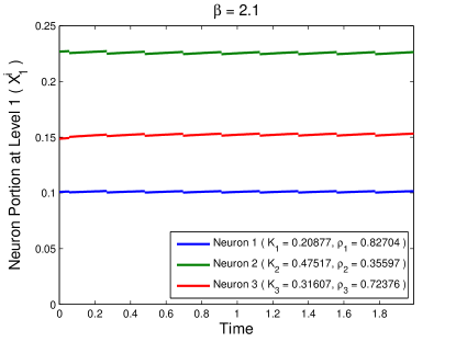
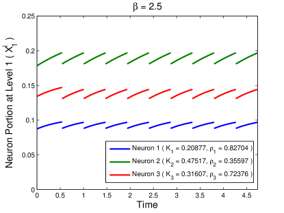
We first numerically solve the hybrid ODE-mapping system, with $M=3$ and random $\alpha_{i},\rho_{i}$. The ODE portion of the hybrid system can be solved explicitly, and we use MATLAB’s fsolve to determine the hitting times $\tau_{i}$. We plot the results for $\beta=2.1$, $\beta=2.5$ for a single initial condition in Figure 3. We observe that each neuron population is attracted to a periodic orbit after several bursts.

Fig. 3: Plots of the hybrid ODE-mapping system numerical simulation results with $\beta=2.1$ (left) and $\beta=2.5$ (right). Both of them are with three neuron populations. The neuron portions at energy level $1$ over simulation time are shown in the plots.

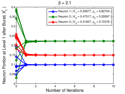
To further demonstrate convergence, we also plot trajectories for the same parameters for various initial conditions in Figure 4. We see that three to four bursts, he trajectories converge to the same periodic orbit.

Fig. 4: Plots of neuron proportions after each burst iteration with $\beta=2.1$ (left) and $\beta=2.5$ (right). Both subfigures are for $M=3$. For all initial conditions, the population seems to converge after about four bursts.

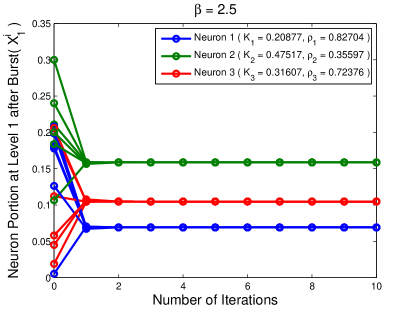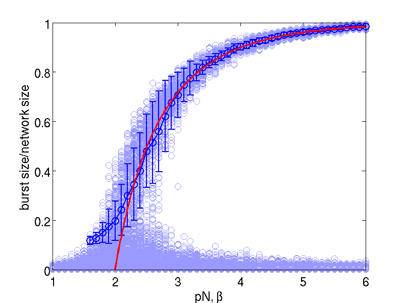
We also study the phase diagram for different $M$, with $\beta$ over the range $[2.005,2.5]$. In the results above, we have only showed that the system converges to the attractor for $\beta>\beta_{M}$, where $\beta_{M}$ might be larger than 2. The numerical evidence in 5 suggests that $\beta_{M}$ might in fact be 2 in general; what we did was choose $1000$ initial conditions at random, and plotted the proportion that fell into each of three categories: those that converged monotonically to a periodic orbit, those that converged non-monotonically to the periodic orbit, and finally, those that did not converge to the periodic orbit. (By converge monotonically, what we mean is that each successive iteration applied to the initial condition was monotonically convergent to the limit and did not overshoot; by non-monotone we mean that the iterations overshot the fixed point.) The third case was always empty, and the only distinction was whether the convergence was monotone or not.

Fig. 5: Phase diagrams for $M=5$ and $M=10$ subpopulations. The parameters $K$ and $\rho$ are chosen at random. For each $\beta,$ we choose $10000$ initial conditions uniformly in the simplex, and determine which proportion falls into each of three categories: monotone convergent, non-monotone convergent and non-convergent. We vary $\beta$ from $2.005$ to $2.5$.

5 Conclusion

We extended the results of [9, 10] to the case of multiple subpopulations with different intrinsic firing rates. We were able to show that the stochastic neuronal network converges to a mean-field limit in general. We further analyzed the limiting mean field in the case where each neuron has at most two inactive states, and proved that for sufficiently large coupling parameters, the mean-field limit has a globally attracting limit cycle. A natural next question to ask is what happens when the system has more inactive states, although the analysis of this higher-dimensional hybrid system is likely to be more difficult (in analogy to the single firing rate case of [10], where the analysis of the mean-field limit was difficult when each neuron had many inactive states).

References

- [1] F. Apfaltrer, C. Ly, and D. Tranchina. Population density methods for stochastic neurons with realistic synaptic kinetics: Firing rate dynamics and fast computational methods. Network-computation in Neural Systems, 17(4):373–418, December 2006.
- [2] Alain Barrat, Marc Barthélemy, and Alessandro Vespignani. Dynamical processes on complex networks. Cambridge University Press, Cambridge, 2008.
- [3] M.S. Branicky. Stability of hybrid systems: state of the art. In Decision and Control, 1997., Proceedings of the 36th IEEE Conference on, volume 1, pages 120–125 vol.1, 1997.
- [4] P. C. Bressloff and S. Coombes. Desynchronization, mode locking, and bursting in strongly coupled integrate-and-fire oscillators. Physical Review Letters, 81(10):2168–2171, September 1998.
- [5] John Buck and Elisabeth Buck. Mechanism of rhythmic synchronous flashing of fireflies. Science, 159(3821):1319–1327, March 22 1968.
- [6] S. R. Campbell, D. L. L. Wang, and C. Jayaprakash. Synchrony and desynchrony in integrate-and-fire oscillators. Neural Computation, 11(7):1595–1619, October 1999.
- [7] Julyan H. E. Cartwright, Victor M. Egu luz, Emilio Hern ndez-Garc a, and Oreste Piro. Dynamics of elastic excitable media. Int. J. of Bifurcation and Chaos, 9(11):2197–2202, 1999.
- [8] C. A. Czeisler, E. Weitzman, M. C. Moore-Ede, J. C. Zimmerman, and R. S. Knauer. Human sleep: its duration and organization depend on its circadian phase. Science, 210(4475):1264–1267, 1980.
- [9] R. E. Lee DeVille and Charles S. Peskin. Synchrony and asynchrony in a fully stochastic neural network. Bull. Math. Bio., 70(6):1608–1633, August 2008.
- [10] R. E. Lee DeVille, Charles S. Peskin, and Joel H. Spencer. Dynamics of stochastic neuronal networks and the connections to random graph theory. Mathematical Modeling of Natural Phenomena, 5(2):26–66, 2010.
- [11] Moez Draief and Laurent Massoulié. Epidemics and rumours in complex networks, volume 369 of London Mathematical Society Lecture Note Series. Cambridge University Press, Cambridge, 2010.
- [12] G. Bard Ermentrout and John Rinzel. Reflected waves in an inhomogeneous excitable medium. SIAM Journal on Applied Mathematics, 56(4):1107–1128, 1996.
- [13] W. Gerstner and J. L. van Hemmen. Coherence and incoherence in a globally-coupled ensemble of pulse-emitting units. Physical Review Letters, 71(3):312–315, July 1993.
- [14] D. T. Gillespie. Master equations for random walks with arbitrary pausing time distributions. Phys. Lett. A, 64(1):22–24, 1977.
- [15] Daniel T. Gillespie. A general method for numerically simulating the stochastic time evolution of coupled chemical reactions. J. Computational Phys., 22(4):403–434, 1976.
- [16] Daniel T. Gillespie. Concerning the validity of the stochastic approach to chemical kinetics. J. Statist. Phys., 16(3):311–318, 1977.
- [17] Daniel T. Gillespie. Monte Carlo simulation of random walks with residence time dependent transition probability rates. J. Comput. Phys., 28(3):395–407, 1978.
- [18] L. Glass, A. L. Goldberger, M. Courtemanche, and A. Shrier. Nonlinear dynamics, chaos and complex cardiac arrhythmias. Proc. Roy. Soc. London Ser. A, 413(1844):9–26, 1987.
- [19] Michael R. Guevara and Leon Glass. Phase locking, period doubling bifurcations and chaos in a mathematical model of a periodically driven oscillator: A theory for the entrainment of biological oscillators and the generation of cardiac dysrhythmias. Journal of Mathematical Biology, 14(1):1–23, March 1982.
- [20] D. Hansel and H. Sompolinsky. Synchronization and computation in a chaotic neural network. Phys. Rev. Lett., 68(5):718–721, Feb 1992.
- [21] E. Haskell, D. Q. Nykamp, and D. Tranchina. Population density methods for large-scale modelling of neuronal networks with realistic synaptic kinetics: cutting the dimension down to size. Network-Computation in Neural Systems, 12(2):141–174, May 2001.
- [22] Raymond Kapral and Kenneth Showalter, editors. Chemical Waves and Patterns. Springer, 1994.
- [23] B. W. Knight. Dynamics of encoding in a population of neurons. Journal of General Physiology, 59(6):734–766, 1972.
- [24] Y. Kuramoto. Collective synchronization of pulse-coupled oscillators and excitable units. Physica D: Nonlinear Phenomena, 50(1):15–30, 1991.
- [25] Thomas G. Kurtz. Relationship between stochastic and deterministic models for chemical reactions. Journal of Chemical Physics, 57(7):2976–2978, 1972.
- [26] Jeffrey C. Lagarias and Yang Wang. The finiteness conjecture for the generalized spectral radius of a set of matrices. Linear Algebra and its Applications, 214(0):17 – 42, 1995.
- [27] D. Liberzon and A.S. Morse. Basic problems in stability and design of switched systems. Control Systems, IEEE, 19(5):59–70, 1999.
- [28] Z.-H. Liu and P.M. Hui. Collective signaling behavior in a networked-oscillator model. Physica A: Statistical Mechanics and its Applications, 383(2):714 – 724, 2007.
- [29] R. E. Mirollo and S. H. Strogatz. Synchronization of pulse-coupled biological oscillators. SIAM J. Appl. Math., 50(6):1645–1662, 1990.
- [30] J. R. Norris. Markov chains, volume 2 of Cambridge Series in Statistical and Probabilistic Mathematics. Cambridge University Press, Cambridge, 1998. Reprint of 1997 original.
- [31] Khashayar Pakdaman and Denis Mestivier. Noise induced synchronization in a neuronal oscillator. Phys. D, 192(1-2):123–137, 2004.
- [32] C. S. Peskin. Mathematical aspects of heart physiology. Courant Institute of Mathematical Sciences New York University, New York, 1975. Notes based on a course given at New York University during the year 1973/74.
- [33] A. Pikovsky, M. Rosenblum, and J. Kurths. Synchronization: A Universal Concept in Nonlinear Sciences. Cambridge University Press, 2003.
- [34] W. Senn and R. Urbanczik. Similar nonleaky integrate-and-fire neurons with instantaneous couplings always synchronize. SIAM J. Appl. Math., 61(4):1143–1155 (electronic), 2000/01.
- [35] Adam Shwartz and Alan Weiss. Large deviations for performance analysis. Chapman & Hall, London, 1995.
- [36] S. Strogatz. Sync: The Emerging Science of Spontaneous Order. Hyperion, 2003.
- [37] D. Terman, N. Kopell, and A. Bose. Dynamics of two mutually coupled slow inhibitory neurons. Phys. D, 117(1-4):241–275, 1998.
- [38] M. Tsodyks, I. Mitkov, and H. Sompolinsky. Pattern of synchrony in inhomogeneous networks of oscillators with pulse interactions. Physical Review Letters, 71(8):1280–1283, August 1993.
- [39] John J. Tyson, Christian I. Hong, C. Dennis Thron, and Bela Novak. A Simple Model of Circadian Rhythms Based on Dimerization and Proteolysis of PER and TIM. Biophys. J., 77(5):2411–2417, 1999.
- [40] John J. Tyson and James P. Keener. Singular perturbation theory of traveling waves in excitable media (a review). Phys. D, 32(3):327–361, 1988.
- [41] C. van Vreeswijk, L. Abbott, and G. Ermentrout. When inhibition not excitation synchronizes neural firing. J. Comp. Neurosci., pages 313–322, 1994.
- [42] C. van Vreeswijk and H. Sompolinsky. Chaotic balance state in a model of cortical circuits. Neural Computation, 10(6):1321–1372, August 15 1998.
- [43] Arthur T. Winfree. The geometry of biological time, volume 12 of Interdisciplinary Applied Mathematics. Springer-Verlag, New York, second edition, 2001.