Abstract

In these lectures we review our present understanding of the fractal structure of two-dimensional Euclidean quantum gravity coupled to matter.

PACS: 04.60.Ds, 04.60.Kz, 04.06.Nc, 04.62.+v.
Keywords: quantum gravity, lower dimensional models, lattice models.

1 Introduction

A noble task in ancient, pre-AdS/CFT time was to find a non-perturbative definition of Polyakov’s bosonic string theory. The formal partition function was defined by the path integral:

$$Z=\int{\cal D}[g_{\alpha\beta}]\;\mbox{e}^{-\Lambda\int d^{2}\!\xi\sqrt{g}}\int{\cal D}_{g}X_{\mu}\;\mbox{e}^{-\frac{1}{2\alpha^{\prime}}\int d^{2}\!\xi\sqrt{g}g^{\alpha\beta}\partial_{\alpha}X_{\mu}\partial_{\beta}X_{\mu}}.$$ (1)

Here $[g_{\alpha\beta}]$ represents a continuous 2d geometry of some fixed topology. Assume that the set of piece-wise linear geometries one can obtain by gluing together equilateral triangles with link length $a$ is uniformly dense in the set of continuous 2d geometries when $a\to 0$. Each such geometry can be identified with an abstract triangulation. By placing the matter field $X_{\mu}(\xi)$ in the center of each triangle and using the natural discretized version of the matter Lagrangian in (1) we obtain a lattice regularization of the action, for which the lattice spacing $a$ acts as a UV cut-off. Summing over the abstract triangulations provides a lattice regularization of the integral over geometries in (1), coined Dynamical Triangulations (DT) [1, 2, 3]. If the assumption about the denseness of these triangulations in the set of continuous geometries holds, we expect to obtain the continuum path integral in the limit $a\to 0$. Of course, it is to be expected that one has to renormalize the bare coupling constants entering in the lattice partition function to recover the continuum results. If we work in units where the lattice spacing $a$ is put to one, we obtain the dimensionless DT partition function

$$Z(\mu)=\sum_{T}\mbox{e}^{-\mu N_{T}}\int^{\prime}\Big{(}\prod_{\triangle\in T}\prod_{\nu=1}^{d}dx_{\nu}(\triangle)\Big{)}\;\mbox{e}^{-\frac{1}{2}\sum_{\triangle,\triangle^{\prime}}(x_{\nu}(\triangle)-x_{\nu}(\triangle^{\prime}))^{2}}$$ (2)

for the bosonic string, where the overall sum is over triangulations $T$ with $N_{T}$ triangles and the sum in the exponent is over pairs $\triangle,\triangle^{\prime}$ of neighboring triangles.

1.1 The free particle

To understand how to obtain the continuum limit of (2), it is useful to study the simpler system of a free particle. In this case the propagator $G(X_{\nu},X^{\prime}_{\nu})$ has the path integral representation

$$G(X_{\nu},X^{\prime}_{\nu})=\int{\cal D}[g]\mbox{e}^{-\Lambda\int d\xi\sqrt{g}}\int{\cal D}_{g}X_{\nu}\;\mbox{e}^{-\frac{1}{2\alpha^{\prime}}\int_{0}^{1}d\xi\sqrt{g}g^{-1}(\partial_{\alpha}X_{\nu})^{2}},$$ (3)

where $X_{\nu}(0)=X_{\nu}$ and $X_{\nu}(1)=X^{\prime}_{\nu}$, and $[g]$ is the geometry of a world line, i.e. $d\ell^{2}=g(\xi)d\xi^{2}$ and $\int d\xi\sqrt{g}=\ell$. The structure of eq. (3) is quite similar to that of eq. (1). The path integral is discretized by dividing the worldline in $n$ equal steps (the equivalent of the equilateral triangles for DT) and using dimensionless variables:

$$G(x_{\nu},x^{\prime}_{\nu},\mu)=\sum_{n}\mbox{e}^{-\mu n}\int\Big{(}\prod_{i=1}^{n}\prod_{\nu=1}^{d}dx_{\nu}(i)\Big{)}\;\mbox{e}^{-\frac{1}{2}\sum_{i=1}^{n}(x_{\nu}(i)-x_{\nu}(i-1))^{2}},$$ (4)

with $x(0)=x$ and $x(n)=x^{\prime}$. One can perform the Gaussian integrations:

$$\int\Big{(}\prod_{i=1}^{n}\prod_{\nu=1}^{d}dx_{\nu}(i)\Big{)}\mbox{e}^{-\frac{1}{2}\sum_{i=1}^{n}(x_{\nu}(i)-x_{\nu}(i-1))^{2}}=\frac{(2\pi)^{nd/2}}{(2\pi n)^{d/2}}\;\mbox{e}^{-\frac{(x_{\nu}-x^{\prime}_{\nu})^{2}}{2n}}.$$ (5)

Introducing $\mu_{c}=\frac{1}{2}d\log(2\pi)$, we get

$$G(x_{\nu},x^{\prime}_{\nu},\mu)=\sum_{n}\frac{1}{(2\pi n)^{d/2}}\;\mbox{e}^{-(\mu-\mu_{c})n}\;\mbox{e}^{-\frac{(x_{\nu}-x^{\prime}_{\nu})^{2}}{2n}},$$ (6)

leading to

$$G(x_{\nu},x^{\prime}_{\nu},\mu)\approx f(|x_{\nu}-x^{\prime}_{\nu}|)\;\;\mbox{e}^{-m(\mu)|x_{\nu}-x^{\prime}_{\nu}|},~{}~{}~{}~{}~{}~{}m(\mu)\propto\sqrt{\mu-\mu_{c}}.$$ (7)

Performing a mass renormalization and a scaling,

$$m^{2}(\mu)=\mu-\mu_{c}=m^{2}_{\textrm{ph}}a^{2},~{}~{}~{}x\,a=X,~{}~{}x^{\prime}\,a=X^{\prime},~{}~{}t=na^{2}$$ (8)

we obtain the standard proper time representation of the free relativistic propagator

$$G(X_{\nu},X^{\prime}_{\nu};m_{\textrm{ph}})=\!\!\lim_{a\to 0}a^{2-d}G(x_{\nu},x^{\prime}_{\nu},\mu)=\!\!\int_{0}^{\infty}\!\!\!\!\frac{dt}{(2\pi t)^{d/2}}\;\mbox{e}^{-m_{\textrm{ph}}^{2}t-\frac{(X_{\nu}-X^{\prime}_{\nu})^{2}}{2t}}.$$ (9)

The explicit, well-defined path integral representation (4) of the free particle is useful for analyzing simple basic properties of the propagator. Let us just mention one such property, the exponential decay of the propagator for large distances. Why can the propagator not fall of faster than exponentially at large distances? The answer is found by looking at Fig. 1. The set of paths from $x$ to $y$ has as a subset the set of paths intersecting the straight line connecting $x$ and $y$ at a point $z$. A path in this subset is a union of a path from $x$ to $z$ and from $z$ to $y$. Since the action for such a path is the sum of the actions of the path from $x$ to $z$ and the path from $z$ to $y$, it is not difficult to show

Figure 1: Decomposition of random walk into two random walks

$$G(x,y)\geq G(x,z)G(z,y),$$ (10)

i.e.

$$-\log G(x,y)\leq-\log G(x,z)-\log G(z,y).$$ (11)

The subadditivity of $-\log G(x,y)$ implies that there exits a positive constant $m$ such that

$$-\log G(x,y)\sim m|x-y|~{}~{}~{}{\rm for}~{}~{}~{}|x-y|\to\infty,$$ (12)

i.e.

$$G(x,y)\sim\mbox{e}^{-m|x-y|}~{}~{}~{}{\rm for}~{}~{}~{}|x-y|\to\infty.$$ (13)

The constant $m$ is the mass of the particle (which can be zero in special cases).

1.2 The bosonic string

One can also perform the Gaussian integration in the string case:

$$\int^{\prime}\!\!\Big{(}\!\prod_{\triangle\in T_{N}}\prod_{\nu=1}^{d}dx_{\nu}(\triangle)\Big{)}\mbox{e}^{-\frac{1}{2}\sum_{\triangle,\triangle^{\prime}}(x_{\nu}(\triangle)-x_{\nu}(\triangle^{\prime}))^{2}}\!=\!\Big{(}\det(-\Delta^{{}^{\prime}}_{T_{N}})\Big{)}^{-d/2}\!,$$ (14)

where $\Delta_{T_{N}}$ is the combinatorial Laplacian on the dual $\phi^{3}$-graph. The prime indicates that the constant zero mode is projected out in the determinant. We find

$$Z(N)=\sum_{T_{N}}\Big{(}\det(-\Delta^{{}^{\prime}}_{T_{N}})\Big{)}^{-d/2}=\mbox{e}^{\mu_{c}N}N^{\gamma(d)-3}\Big{(}1+{\cal O}\Big{(}\frac{1}{N^{2}}\Big{)}\Big{)}$$ (15)

and

$$Z(\mu)=\sum_{N}\mbox{e}^{-\mu N}Z(N)=\sum_{N}\mbox{e}^{-(\mu-\mu_{c})N}N^{\gamma(d)-3}\Big{(}1+{\cal O}\Big{(}\frac{1}{N^{2}}\Big{)}\Big{)}.$$ (16)

In the scaling limit $\mu\to\mu_{c}$ one may identify

$$\mu-\mu_{c}=\Lambda a^{2},~{}~{}~{}(\mu-\mu_{c})N_{T}=\Lambda\int d^{2}\xi\sqrt{g}.$$ (17)

Equation (16) is valid for geometries with fixed topology of the sphere, but $Z(\mu)$ generalizes naturally to surfaces with $n$ boundaries $\{\gamma_{i}\}$ of fixed length $L_{i}$ on which the coordinates $x_{\mu}$ are fixed. In particular, in the limit $L_{i}\to 0$ we obtain the $n$-point function $G(x_{1},\ldots,x_{n};\mu)$ for spherical string world sheets with $n$ marked points at prescribed positions $x_{1},\ldots,x_{n}$.

A basic property of the two-point function $G(x_{1},x_{2};\mu)$ is subadditivity. The argument is essentially the same as for the particle, except that random surfaces are involved instead of random walks, as illustrated in Fig. 2.

Figure 2: Subadditivity of the string two-point function.

Therefore we find

$$G(x_{1},x_{2};\mu)\sim\mbox{e}^{-m(\mu)|x_{1}-x_{2}|},~{}~{}~{}~{}~{}m(\mu)\geq 0.\$$ (18)

Similarly we may consider the planar “Wilson loop” $G(\gamma_{L_{1}\times L_{2}},\mu)$, corresponding to the partition function with one boundary $\gamma_{L_{1}\times L_{2}}$ of length $2L_{1}+2L_{2}$ corresponding to a rectangular loop in $\mathbb{R}^{d}$ with sides of length $L_{1}$ and $L_{2}$. As illustrated in Fig. 3, $G(\gamma_{L_{1}\times L_{2}},\mu)$ is subadditive both in $L_{1}$ and $L_{2}$, and therefore we obtain

$$G(\gamma_{L_{1}\times L_{2}},\mu)\sim\mbox{e}^{-\sigma(\mu)A(\gamma_{L_{1}\times L_{2}})},~{}~{}~{}~{}\sigma(\mu)\geq 0,$$ (19)

where $A(\gamma_{L_{1}\times L_{2}})=L_{1}L_{2}$ is the area of the loop, and $\sigma(\mu)$ is known as the string tension.

Figure 3: Subadditivity of the Wilson loop.

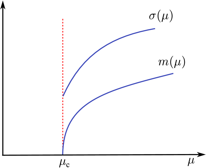
However, the dominant worldsheet surfaces look completely different from the nice surfaces shown in Fig. 2 and Fig. 3. The reason for this is shown in Fig. 4. It is seen from the figure that, while the mass of the two point function scales to zero at a critical point, which is needed if one wants a continuum limit, this is not the case for the string tension $\sigma(\mu)$ ([5] or [4], theorem 3.6). The consequence is that the physical string tension scales to infinity as $\mu\to\mu_{c}$:

$$m(\mu)=(\mu-\mu_{c})^{\nu}=m_{\textrm{ph}}\,a^{\nu},~{}~{}~{}~{}\sigma(\mu)=\sigma_{\textrm{ph}}\,a^{2\nu},~{}~{}~{}\sigma_{\textrm{ph}}\to\infty.$$ (20)

Figure 4: The scaling of the bare mass and the bare string tension as a function of the bare coupling constant $\mu$.

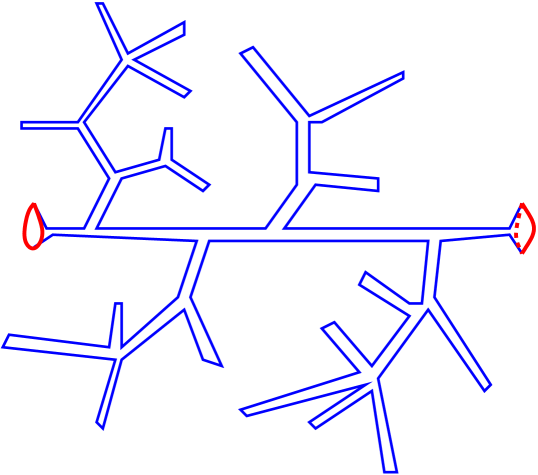
An infinite string tension implies that any surface with finite area is forbidden unless it is dictated by some imposed boundary conditions. A typical surface with no area contributing to the two-point function $G(x_{1},x_{2},\mu)$ is shown in Fig. 5. Such surfaces are called branched polymer (BP) surfaces. They have only one mass excitation corresponding to a free particle, since one basically obtains a random walk representation corresponding to the free particle by scaling away the branches decorating the shortest path from $x_{1}$ to $x_{2}$ for a given surface connecting $x_{1}$ and $x_{2}$.

Figure 5: Branched polymer surfaces dominate the bosonic string two-point function.

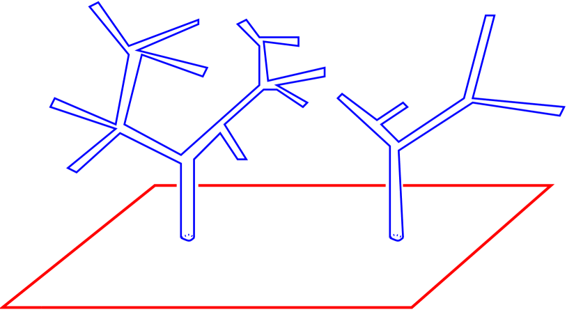
In the case of the Wilson loop we are summing over surfaces where the boundary is fixed. Therefore we have a minimal-area surface stretching to the boundary. The fluctuations around this surface, however, are again branched polymers, as shown in Fig. 6, and are nothing like the surface in Fig. 3.

Figure 6: The fluctuations around the minimal surface in the path integral of the Wilson loop are of the form of branched polymers.

The conclusion is that the bosonic string theory defined through a regulated path integral where all surfaces have positive weight does not exist. The reason that we do not obtain the standard bosonic string, despite such a well-defined procedure, is that the two-point function of the standard bosonic string has tachyonic mass excitations, which are excluded by our construction and which make standard bosonic string theory sick.

2 Non-critical string theory

However, interpreting the string world sheet as 2d space-time, we can view Polyakov’s bosonic string theory in $d$ dimensions as 2d gravity coupled to $d$ massless scalar fields, i.e. to a conformal field theory with central charge $c=d$. Therefore, as another route towards the bosonic string, we can study 2d quantum gravity coupled to (conformal) field theories. Surprisingly this theory, called non-critical string theory, has a rich structure as long as the central charge $c\leq 1$.

The regularized version of such a theory is typically obtained as follows: assume we have a conformal field theory originating from a field theory on a regular lattice. Usually the lattice theory has a critical point with a second-order phase transition and the continuum conformal field theory is then defined at the critical point. This lattice field theory can usually be transfered from a regular lattice to a random one, hence, also to the random lattice appearing in the DT formalism.

Including a summation over different lattices in ensemble averages is what is called an annealed average in the context of condensed matter physics. Here it will play the role of integrating over 2d geometries, as for the bosonic string.

The partition function of 2d gravity coupled to matter can be written as

$$Z=\sum_{N}\mbox{e}^{-\mu N}\sum_{T_{N}}Z_{T_{N}}({\rm matter}),$$ (21)

where $Z_{T_{N}}({\rm matter})$ is the matter partition function on a fixed triangulation $T_{N}$. A typical example is the Ising model coupled to DT [6],

$$Z_{T_{N}}(\beta)=\sum_{\sigma_{\triangle}=\pm 1}\exp\Big{[}\beta\sum_{\triangle,\triangle^{\prime}}\;\sigma_{\triangle}\sigma_{\triangle^{\prime}}\Big{]}.$$ (22)

The partition function scales as

$$Z_{N}(\beta)=\sum_{T_{N}}Z_{T_{N}}(\beta)=\mbox{e}^{\mu_{c}(\beta)N}\,N^{\gamma(\beta)-3}\Big{(}1+O(N^{-2})\Big{)},$$ (23)

$$Z(\beta)=\sum_{N}\mbox{e}^{-\mu N}Z_{N}(\beta)=\sum_{N}\mbox{e}^{-(\mu-\mu_{c}(\beta))N}N^{\gamma(\beta)-3}(1+\cdots).$$ (24)

Here $\mu_{c}(\beta)$ appears as the critical “cosmological” constant for the geometries, such that one obtains universes with infinitely many triangles when $\mu\to\mu_{c}$ from above. This is similar to the situation for the free particle and the bosonic string and we clearly want to take that limit in order to recover continuum physics from the lattice theory. However, it also follows from (23) that it has the interpretation as the the free energy density of spins in the annealed ensemble.

The model has a phase transition at a critical $\beta_{c}$, the transition being third order rather than the standard second order phase transition [6]. At the transition point $\gamma(\beta)$ jumps from -1/2 to -1/3. The interpretation is as follows: on a regular lattice the Ising spin system also has a phase transition at a certain critical temperature $\beta_{c}$. The transition is a second order transition and at the transition point the spin system describes the continuum conformal field theory of central charge $c=1/2$. The lattice theory, defined on the annealed average of lattices, describes at its critical point the $c=1/2$ conformal field theory coupled to 2d quantum gravity, the average over the DT lattices being the path integral over geometries. It is not surprising that the transition can change from a second order to a third order transition, the randomness of the lattices and the averaging over different lattices making it more difficult to build up large critical spin clusters at the phase transition point. Maybe it is more surprising that there is a transition at all. But it is known to be the case, since one can solve the model analytically. One finds that the critical spin exponents have changed compared to Onsager exponents on a regular lattice. Thus the continuum conformal field theory has changed due to the interaction with 2d quantum gravity. Further, as we mentioned, the exponent $\gamma(\beta)$ jumps at $\beta_{c}$. The exponent $\gamma(\beta)$ as it appears in (24) reflects average fractal geometric properties of the ensemble of random geometries appearing in the path integral. Thus a change in the exponent reflects that the conformal field theory back-reacts on the geometry and changes its fractal properties, something we will discuss in detail below. Away from $\beta_{c}$ the Ising model is not critical, and the lattice spins couple only weakly to the lattice. For all $\beta\neq\beta_{c}$ one has $\gamma(\beta)=-1/2$ and this can then be viewed as the exponent for “pure 2d Euclidean gravity” without matter fields.

2.1 Continuum formulation

One can study 2d quantum gravity coupled to matter fields entirely in the continuum. Just like for the partition function (1) for the bosonic string, we can write formally

$$Z=\int{\cal D}[g_{\alpha\beta}]\;\mbox{e}^{-\Lambda A(g)}\int{\cal D}_{g}\psi\;\mbox{e}^{-S(\psi,g)},~{}~{}~{}~{}A(g)=\int d^{2}\xi\,\sqrt{g},$$ (25)

where $\psi$ represents some matter field. A partial gauge fixing, to the so-called conformal gauge $g_{\alpha\beta}=\mbox{e}^{\phi}{\hat{g}}(\tau_{i})$ leads to

$$Z({\hat{g}})=\int{\cal D}_{{\hat{g}}}\phi\,\mbox{e}^{-S_{L}(\phi,{\hat{g}})},$$ (26)

where $S_{L}(\phi,{\hat{g}})$ is fixed by the requirement that $Z({\hat{g}})$ is independent of ${\hat{g}}$, namely [8]

$$S_{L}(\phi,{\hat{g}})=\frac{1}{4\pi}\int d^{2}\xi\sqrt{{\hat{g}}}\;\Big{(}(\partial_{\alpha}\phi)^{2}+Q\,\hat{R}\,\phi+\mu\,\mbox{e}^{2\beta\phi}\Big{)},$$ (27)

$$Q=\sqrt{(25-c)/6},~{}~{}~{}~{}Q=1/\beta+\beta.$$ (28)

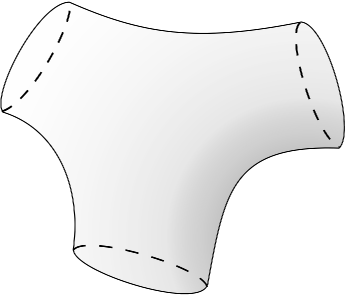
Even for $c=0$ we have a non-trivial theory. The $c=0$ partition function can be obtained explicitly at the regularized level simply by counting the triangulations, since there are no matter fields. A slightly non-trivial structure can be imposed by $n$ boundaries of lengths $\ell_{n}$, as illustrated in Fig. 7 for the case $n=3$. Also in that case the counting can be done and the continuum limit taken.

Figure 7: The 3-loop function

The continuum definitions of the $n$-loop functions are

$$W(\ell_{1},\ldots,\ell_{n},V)\!\! = \int_{\ell_{1},\ldots,\ell_{n}}{\cal D}[g_{\alpha\beta}]\;\delta(A(g)-V),$$ (29)

$$W(\ell_{1},\ldots,\ell_{n},\Lambda)\!\! = \int_{\ell_{1},\ldots,\ell_{n}}{\cal D}[g_{\alpha\beta}]\;\mbox{e}^{-\Lambda A(g)},$$ (30)

$$W(\Lambda^{B}_{1},\ldots,\Lambda^{B}_{n},\Lambda)\!\! = \int{\cal D}[g_{\alpha\beta}]\;\mbox{e}^{-\Lambda A(g)-\sum_{i}\Lambda_{i}^{B}\ell_{i}(g)}.$$ (31)

Formally (29) counts each continuous geometry (defined by an equivalence class of metrics $[g_{\alpha\beta}(\xi)]$) with weight one. Eq. (30) defines the partition function for universes with fixed boundary lengths $\ell_{i}$ and with a cosmological constant $\Lambda$. Eq. (31) defines the partition function for universes with boundary cosmological constants $\Lambda^{B}_{i}$ and bulk cosmological constant $\Lambda$, i.e. the partition function where both the lengths of the boundaries and the size of the universe are allowed to fluctuate, controlled by the various cosmological constants. From a “counting perspective” one can view $W(\Lambda^{B}_{1},\ldots,\Lambda^{B}_{n},\Lambda)$ as the generating function for $W(\ell_{1},\ldots,\ell_{n},V)$, the number of continuous geometries with $n$ boundaries of lengths $\ell_{i}$.

Of course, to perform any real counting one has to introduce a regularization such that one starts out with a finite number of geometries, and for this purpose the DT-formalism is perfect. As an example we can write the regularized DT version of $W(\Lambda^{B},\Lambda)$, i.e. the 1-loop function, as

$$W(z_{1},g)=\frac{1}{z_{1}}\sum_{k,l_{1}}W(l_{1},k)\;g^{k}z_{1}^{-l_{1}},~{}~{}~{}g=\mbox{e}^{-\mu},~{}z_{1}=\mbox{e}^{\lambda_{1}},$$ (32)

such that $W(z_{1},g)$ is the generation function for $W(l_{1},k)$, the number of triangulations with $k$ triangles and a boundary with $l_{1}$ links. As with most counting problems, it is easier first to find the generating function $W(z_{1},g)$ and then by inverse (discrete) Laplace transformations to find the numbers $W(l_{1},k)$.

The result of this counting ([7], see [4], Chapter 4, for a review) is that after the continuum limit is taken, using the techniques of renormalization of the bare lattice cosmological constant $\mu$ and boundary cosmological constants $\lambda_{i}$ (appearing in (32)), one obtains the expression

$$W(\ell_{1},\ldots,\ell_{n},V)=V^{n-7/2}\sqrt{\ell_{1}\cdots\ell_{n}}\;\mbox{e}^{-(\ell_{1}+\cdots+\ell_{n})^{2}/V}.$$ (33)

Starting out from the continuum Liouville theory the same result has been reproduced. In this sense the agreement shows that the DT lattice regularization works perfectly (and even allows one to perform certain analytic calculation with less effort than using the continuum formulation, something very rare for a lattice regularization). It also gives additional confidence in the continuum Liouville calculations, which rely on certain bootstrap assumptions about conformal invariance.

3 The fractal structure of 2d QG

While eq. (33) is an amazing formula, basically counting the number of continuous 2d geometries with the topology of a sphere with $n$ boundaries, it tells us little about the “typical” 2d continuous geometry one encounters in the path integral. In order to probe such a geometry we need some specific reference to distance. One could be worried that it makes no sense to talk about distance in a theory of quantum gravity, i.e. a theory of fluctuating geometry, since it is precisely the geometry that defines distance. However, the key message of the following is that it does make sense to talk about geodesic distance even in a such a theory.

Let us define the two-point function $G(R;V)$ of geodesic distance $R$ for surfaces of fixed volume $V$ by

$$G(R;V)=$$

$$\int\!{\cal D}[g]\!\int\!{\cal D}_{g}\psi\;\mbox{e}^{-S[g,\psi]}\;\delta\Big{(}A(g)\!-\!V\Big{)}\!\!\int\!\!dx\sqrt{g(x)}\!\!\int\!\!dy\sqrt{g(y)}\;\delta(R\!-\!D_{g}(x,y)),$$

where $A(g)\equiv\int d^{2}x\sqrt{g(x)}$ and $D_{g}(x,y)$ denotes the geodesic distance between $x$ and $y$ in the geometry defined by the metric $g_{\alpha\beta}(x)$. The defining formula (3) is valid for any matter field $\psi$ coupled to 2d quantum gravity. In principle it is also valid in a higher dimensional theory of quantum gravity provided one includes in $S[g,\psi]$ the Einstein action (or whatever one uses as the action). In two dimensions the Einstein action is topological and we may drop it.

It might be convenient not to keep $V$ fixed, but rather to consider the two-point function for the ensemble of universes with a fixed cosmological constant $\Lambda$, i.e.

$$G(R;\Lambda)=\int_{0}^{\infty}dV\;\mbox{e}^{-\Lambda\,V}\;G(R;V).$$ (35)

These two-point functions probe the geometries in the following way. Denote the “area” of a spherical shell at geodesic distance $R$ from point $x$ by

$$S_{V}(x;R)=\int dy\sqrt{g(y)}\;\delta(D_{g}(x,y)-R),$$ (36)

which, of course, depends both on the chosen geometry $g_{\alpha\beta}$ and the point $x$. Let us denote the diffeomorphism invariant average of $S_{V}(x;R)$ by

$$S_{V}(R)=\frac{1}{V}\int dx\sqrt{g(x)}\;S_{V}(x;R).$$ (37)

The quantum average of $S_{V}(R)$ over all geometries is then related to $G(R;V)$ by

$$\langle S_{V}(R)\rangle=\frac{1}{VZ(V)}\;G(R;V),$$ (38)

where $Z_{V}$ is the corresponding partition function of 2d quantum gravity coupled to matter, i.e. the rhs of (3) but with the integral (and integrand) over $x,y$ removed. For a smooth 2d geometry we have

$$S_{V}(R)\sim R,~{}~{}~{}{\rm for}~{}~{}~{}R\ll V^{1/2},$$ (39)

while in general we define the fractal dimension, or Hausdorff dimension, $d_{h}$ for the quantum average by

$$\langle S_{V}(R)\rangle\sim R^{d_{h}-1}~{}~{}~{}{\rm for}~{}~{}~{}R\ll V^{1/d_{h}}.$$ (40)

The partition function scales as $Z(V)\sim V^{\gamma(c)-3}$, where the string susceptibility $\gamma(c)$ is a function of the central charge $c$ of the matter field coupled to the geometry and is known to be given by [8, 9]

$$\gamma(c)=\frac{c-1-\sqrt{(c-1)(c-25)}}{12}.$$ (41)

In the absence of matter fields, i.e. $c=0$, we have $\gamma=-1/2$, and the scaling is seen to agree with (33) for $n=0$. Therefore we can determine $d_{h}$ from the functional form of $G(R;V)$ or $G(R;\Lambda)$. Remarkably, there is a simple and closed formula for $G(R;\Lambda)$ for $c=0$, obtained again by counting triangulations, namely [11]

$$G(R;\Lambda)=\Lambda^{3/4}\;\frac{\cosh(\sqrt[4]{\Lambda}\;R)}{\sinh^{3}(\sqrt[4]{\Lambda}\;R)}.$$ (42)

This can be turned into an expression for $G(R;V)$ by an inverse Laplace transformation, which may plugged into (40), leading to

$$\langle S_{V}(R)\rangle=R^{3}F\left(\frac{R}{V^{1/4}}\right),~{}~{}~{}F(0)>0,$$ (43)

where $F(x)$ is a hypergeometric function falling off for large $x$ as $e^{-x^{4/3}}$. Note that, while $G(R;V)$ falls of faster than exponentially as a function of $R$, this is not possible for $G(R;\Lambda)$ because of arguments of subadditivity of the kind already used for the two-point function of the bosonic string.

Comparing (43) to (40), we conclude that 2d continuous geometry is fractal with Hausdorff dimension $d_{h}=4$ [10, 12]. This is in some sense similar to the situation for the free particle, where one is summing over continuous path from $x$ to $y$ in $\mathbb{R}^{d}$. There a typical path is not a one-dimensional object, but is fractal with $d_{h}=2$. The difference is that for the geometries we have no embedding space $\mathbb{R}^{d}$ with respect to which we can define a distance. This makes it the more remarkable that one still has a concept of geodesic distance that survives the averaging over all geometries.

Figure 8: The fractal structure of a “typical” 2d geometry.

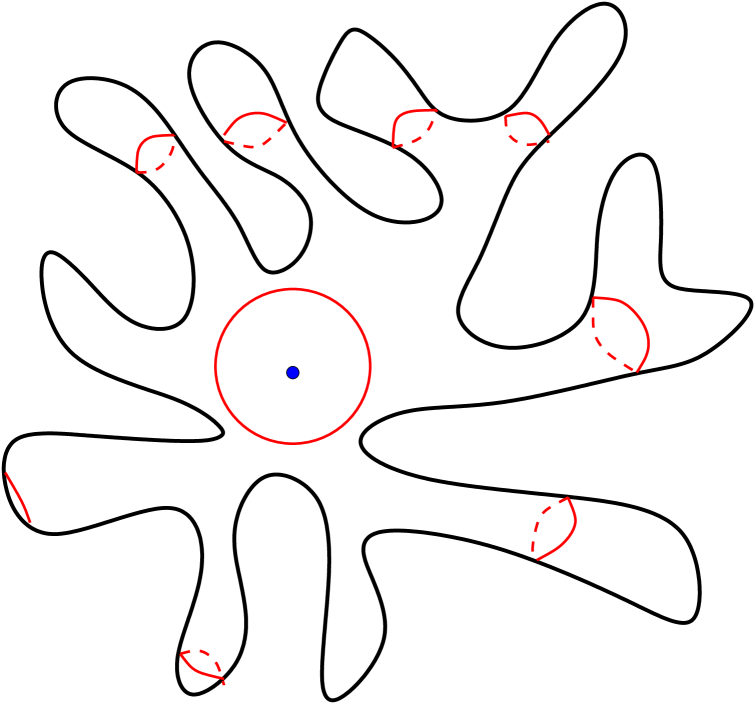
How is it possible that $d_{h}=4$? The reason $d_{h}$ can be larger than 2 is that $S_{V}(x;R)$ is almost surely not connected, as is illustrated in Fig. 8. In fact, one can show [11] that the number of connected components of $S_{V}(x;R)$ with length $\ell$ between $\ell$ and $\ell+d\ell$ is given by

$$\rho_{R}(\ell)\propto\frac{1}{R^{2}}\left(y^{-5/2}+\frac{1}{2}y^{-3/2}+\frac{14}{3}y^{-1/2}\right)\,\mbox{e}^{-y},~{}~{}~{}~{}y=\frac{\ell}{R^{2}},$$ (44)

in the limit $V\to\infty$. Thus the number of components with small $\ell$ diverges for $\ell\to 0$. Of course, in the DT formalism there is a cut-off in the sense that the smallest loop length consists of a single link (of length $a$, the UV cut-off). In the presence of such a cut-off (44) leads to

$$\langle S_{V\to\infty}(R)\rangle=\int_{a}^{\infty}d\ell\;\ell\;\rho_{R}(\ell)\propto\frac{R^{3}}{\sqrt{a}},$$ (45)

again leading to the conclusion that $d_{h}=4$.

3.1 The central charge different from zero

For $c\neq 0$ (and $c\leq 1$) no detailed calculations exist like the ones reported above. However, there exists a remarkable formula derived by Watabiki [13] for $d_{h}$ for any $c\leq 1$:

$$d_{h}(c)=2\frac{\sqrt{49-c}+\sqrt{25-c}}{\sqrt{25-c}+\sqrt{1-c}},~{}~{}~{}~{}~{}~{}~{}~{}~{}d_{h}(0)=4,~{}~{}~{}~{}d_{h}(-\infty)=2.$$ (46)

The formula was derived by applying scaling arguments, which we will briefly summarize, to diffusion on two-dimensional geometries in quantum Liouville theory.

Let $\Phi_{n}[g]$ be a functional of the metric which is invariant under diffeomorphisms and assume that classically $\Phi_{n}[\lambda g]=\lambda^{-n}\Phi[g]$ for constant $\lambda$. According to the KPZ relations the quantum average then satisfies [14, 8, 13]

$$\langle\Phi[g]\rangle_{\lambda V}=\lambda^{-\alpha_{-n}/\alpha_{1}}\langle\Phi[g]\rangle_{V},~{}~{}~{}~{}~{}\alpha_{n}=\frac{2n}{1+\sqrt{\frac{25-c-24n}{25-c}}}$$ (47)

One now applies this to the operator

$$\Phi_{1}[g]=\int dx\sqrt{g}\;\left[\Delta_{g}(x)\;\delta_{g}(x,x_{0})\right]_{x=x_{0}},~{}~{}~{}~{}\Phi_{1}[\lambda g]=\lambda^{-1}\Phi_{1}[g],$$ (48)

which appears when we study diffusion on a smooth manifold with metric $g_{\mu\nu}$. The diffusion kernel is

$$K(x,x_{0};t)=\mbox{e}^{t\Delta_{g}}\,K(x,x_{0};t),~{}~{}~{}~{}K(x,x_{0};0)=\delta_{g}(x,x_{0}).$$ (49)

It has short distance behavior

$$K(x,x_{0};t)\sim\frac{\mbox{e}^{-D^{2}(x,x_{0})/2t}}{t^{d/2}}\,(1+{\cal O}(t)),~{}~{}~{}~{}~{}\langle D(x,x_{0};t)^{2}\rangle\sim t+{\cal O}(t^{2}).$$ (50)

The return probability is defined in terms of the diffusion kernel as

$$P(t) = \frac{1}{V}\int dx\sqrt{g}\;K(x,x;t)$$ (51)

$$= \frac{1}{V}\int dx\sqrt{g}\left[(1+t\Delta_{g}+\cdots)\;\delta_{g}(x-x_{0})\right]_{x=x_{0}}$$

$$= c+t\,\Phi_{1}[g]+O(t^{2})$$

These equations are trivially correct for a smooth geometry $g_{\alpha\beta}(x)$, and they link the dimension of $\Phi_{1}[g]$ to the dimension of $D(x,x_{0})$:

$${\rm Dim}[D(x,x_{0})]=-\frac{1}{2}{\rm Dim}[\Phi[g]].$$ (52)

Of course, this link is trivial in the sense that ${\rm Dim}[D(x,x_{0})]=1$ and ${\rm Dim}[\Phi_{1}[g]]=-2$ by construction. Watabiki now conjectured that (52) survives the quantum averaging, where we know from (47) how the dimension of $\Phi_{1}[g]$ changes. Thus one obtains

$${\rm Dim}[\langle D(x,x_{0})\rangle]=-\frac{1}{2}{\rm Dim}[\langle\Phi[g]\rangle]=-\frac{\alpha_{-1}}{\alpha_{1}},$$ (53)

leading to (46) if we declare that Dim[$V$] = 2, such that

$$\langle V\rangle_{R}=R^{d_{h}},~{}~{}~{}~{}~{}~{}{\rm Dim}[R]=\frac{2}{d_{h}}.$$ (54)

3.2 Is the Watabiki formula correct?

One may be worried about the previous derivation of $d_{h}(c)$, since the result implies that a typical spacetime is fractal, while the basic relation used, namely (51), is valid only on smooth spacetimes. But not only that: numerical simulations [15] seem to show that the diffusion distance $R(t)$ scales like $\langle R^{2}(t)\rangle\sim t^{2/d_{h}}$, rather than like in (50). Anomalous diffusion is normal on fractal spacetimes, but it makes the Watabiki derivation problematic. Nevertheless, the predicted $d_{h}(0)$ is clearly correct and it might be that $d_{h}(c)$ is also correct for $c\neq 0$. This is what we have tried to test using numerical methods to measure $d_{h}(c)$.

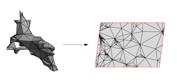
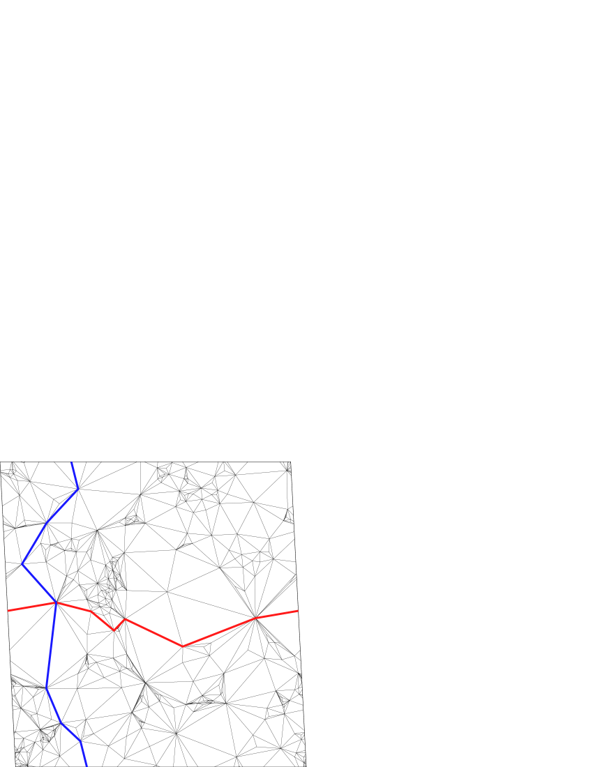
We have found it convenient to use 2d spacetimes with toroidal topology. These have the virtue that their shortest non-contractible loop is automatically a geodesic curve [18]. Thus in the discretized case we only have to look for such loops. Further, the harmonic forms which are important tools for analytic manifolds have very nice discretized analogies, and we can use the these to construct a conformal mapping from the abstract triangulation to the complex plane [16, 17]. We have shown an example of such a map in Fig. 9.

Figure 9: Example of a discrete analog of a harmonic map, used to map a triangulation of the torus consisting of equilateral triangles into the complex plane [16].

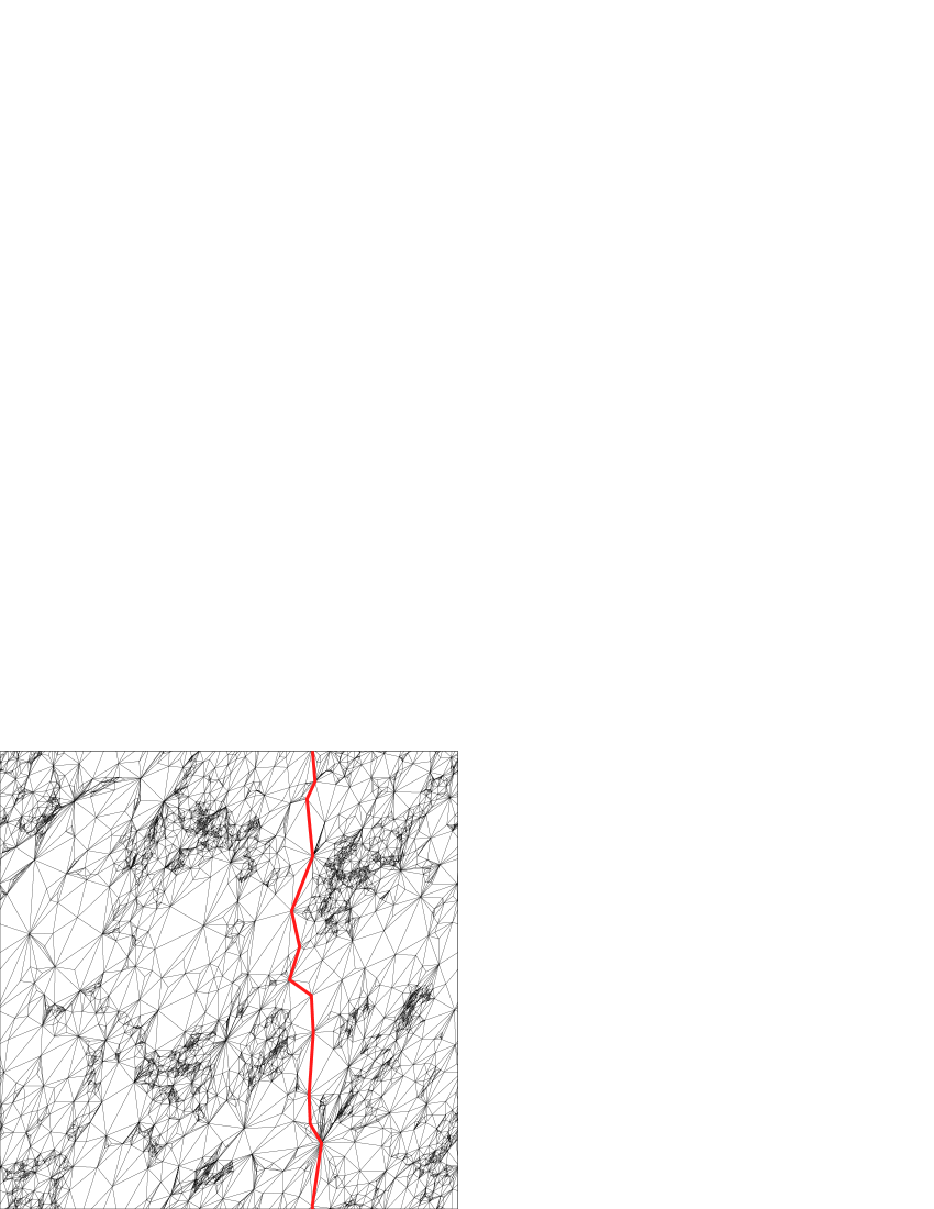
Since the shortest non-contractible loop is a geodesic we expect

$$\langle L\rangle_{N}\sim N^{1/d_{h}(c)}$$ (55)

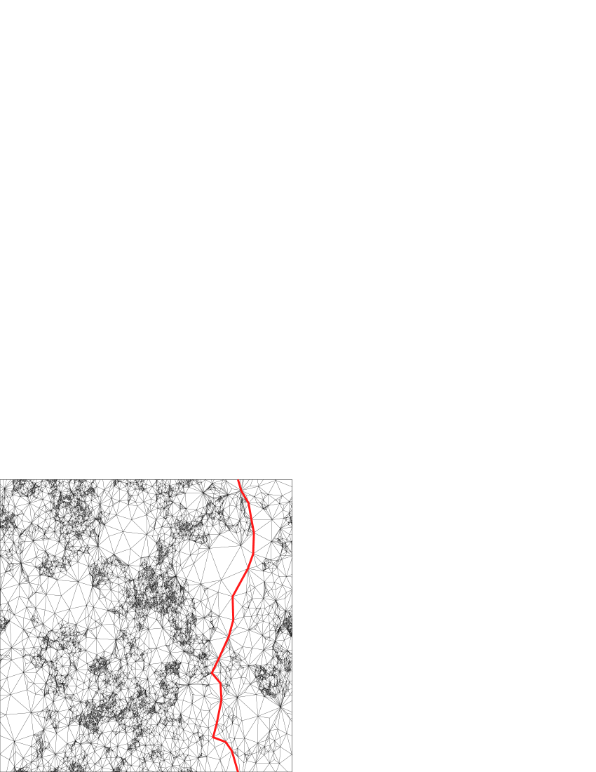
An amazing qualitative test of this is shown in Fig. 10, where we use the harmonic map mentioned to map two abstract triangulations corresponding to $c=0$ and $c=-2$ and 150000 triangles into the complex plane. Already just by looking at the figures one can basically verify qualitatively (55).

  

Figure 10: The left figure corresponds to $c=0$, i.e. $d_{h}=4$, and the right figure to $c=-2$, i.e. $d_{h}=3.56$. The shortest path non-contractible loop is shown in both cases [16].

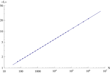
A quantitative check of $\langle L\rangle_{N}\sim N^{1/d_{h}}$ for $c=-2$ is shown in Fig. 11, where we have averaged over many configurations for a fixed size $N$ of the triangulation, and performed the measurements of the shortest non-contractible loops for different sizes $N$. Formula (46) seems very well satisfied numerically for $c=-2$.

Figure 11: The numerical expectation value $\langle L\rangle_{N}$ of the length of the shortest non-contractible loop for triangulations of $N$ triangles (the error bars are too small to display). The fit corresponds to $\langle L\rangle_{N}=0.45\;N^{1/3.56}$ [16].

Recall that the partition function for the (regularized) bosonic string embedded in $d$ dimensions is given by eq. (14): it can be viewed as a conformal field theory with central charge $c=d$ coupled to 2d quantum gravity. As we have seen, the theory degenerates into BP for $c>1$. However, from (14) it is clear that we can formally perform an analytic continuation to $c<1$. A special case is $c=-2$ because then the triangulations are weighted precisely by the determinant of the graph Laplacian, which can be represented as a sum over spanning trees of the given triangulations. This fact was used in the numerical simulations reported above and allowed us to sample very large triangulations and to obtain great numerical accuracy [16].

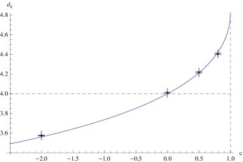
More generally one can sample from the partition function for any fixed real value $c$ by explicitly evaluating the determinant in a Monte Carlo simulation [19]. This can, of course, only be done efficiently for relatively small triangulations. However, it turns out that to study DT for large negative $c\ll-2$ and to obtain a qualitative verification of formula (46), one only requires such small triangulations. In particular, the formula tells us that $d_{h}\to 2$ for large negative $c$, indicating that nice smooth geometries should dominate in that limit. This is illustrated in Fig. 12.

Figure 12: Qualitative agreement with (46) for large negative $c$ [19].

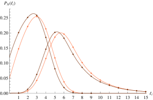
The situation for $c>0$ is more difficult and until recently numerical simulations could not really determine $d_{h}(c)$ properly for $c>0$. Matter correlation functions gave agreement with Watabiki’s formula, but geometric measurements agreed better with $d_{h}=4$ for $0<c<1$. Recently simulations have been performed of DT on the torus coupled to the Ising model ($c=1/2$) and the 3-states Potts model ($c=4/5$) [20]. In addition to the shortest non-contractible loop length $\ell_{0}$, also the length $\ell_{1}$ of the second shortest independent loop was analyzed (see Fig. 13), yielding data with little discretization “noise”.

Figure 13: Example of two shortest, independent loops [20].

The probability distributions for the lengths $\ell_{i}$ are expected, for large $N$, to be of the form

$$P_{N}^{(i)}(\ell_{i})=N^{1/d_{h}}F_{i}(x_{i})~{}~{}~{}~{}x_{i}=\frac{\ell_{i}}{N^{1/d_{h}}}$$ (56)

By measuring the distributions for various $N$’s and attempting to “collapse” the distributions to the common, universal functions $F_{i}(x_{i})$ we can determine $d_{h}$. Typically, one chooses reference distributions, here chosen to be interpolations of the loop length distributions for $N=8000$, to which the data for the other system sizes is fitted. In Fig. 13 the reference distributions $P_{N}(\ell_{0})$ and $P_{N}(\ell_{1})$ are plotted for both the Ising model and the 3-states Potts model. It is seen that the second shortest loop distributions contain less very short loops, which is probably why their lengths have less discretization effects and show better scaling.

Figure 14: The reference distributions $P_{N}(\ell_{0})$ (left) and $P_{N}(\ell_{1})$ (right) for the Ising model (light curves) and the 3-states Potts models (dark curves) extracted from the data at $N=8000$ [20].

The best fits of $d_{h}$ for the data are shown in Fig. 15 and summarized in the following table.

Figure 15: The results of high precision measurements of $d_{h}(c)$ [20]. The shown curve is $d_{h}(c)$ as defined by eq. (46), and the measurements are for $c=-2,0,1/2,4/5$.

$c$	$d_{h}$ (by fit)	$d_{h}$ (theoretical)
$-2$	$3.575\pm 0.003$	$3.562$
$0$	$4.009\pm 0.005$	$4.000$
$1/2$	$4.217\pm 0.006$	$4.212$
$4/5$	$4.406\pm 0.007$	$4.421$

4 Matter correlation functions

We have seen that the two-point functions $G(R;\Lambda)$ and $G(R;V)$ are good probes of the quantum geometry of 2d spacetime and allowed us to define the concept of an average geodesic distance. Also for matter correlators $\langle\phi(x)\phi(y)\rangle$ the first obvious question one can ask is whether it makes any sense to talk about such correlators as functions of distance, and which distance should one use if we are integrating over all geometries? It is natural to define the diffeomorphism invariant matter correlators as the following generalization of eq. (3) for $G(R;V)$:

$$\langle\phi\phi(R)\rangle_{V} = \frac{1}{Z_{V}}\int\!{\cal D}[g]\!\int\!{\cal D}_{g}\phi\;\mbox{e}^{-S[g,\phi]}\;\delta\Big{(}A(g)\!-\!V\Big{)}$$

$$\int\!\!\int\!\!dx\,dy\;\frac{\sqrt{g(x)}\,\sqrt{g(y)}}{S_{g}(y,R)\;V}\;\phi(x)\,\phi(y)\;\delta(R\!-\!D_{g}(x,y)).$$

It is a non-local definition of a matter correlator, but there exists no diffeomorphism invariant local definition.

Assume we consider a conformal field theory in flat spacetime and let $\phi(x)$ be a primary operator with scaling dimension $\Delta_{0}$. We thus have the following behavior of the $\phi\!-\!\phi$ correlator

$$\langle\phi(x)\phi(y)\rangle\sim|x-y|^{-2\Delta_{0}}.$$ (58)

If we take the quantum average as in (4) the geodesic distance $R$ scales anomalously and we expect for dimensional reasons that $|x-y|^{-2}$ is replaced by $R^{-d_{h}}$. However, we also know from KPZ scaling that the scaling dimension $\Delta_{0}$ of $\phi$ will be changed after coupling to 2d quantum gravity such that

$$\Delta(c)=2\;\frac{\sqrt{1-c+12\Delta_{0}}-\sqrt{1-c}}{\sqrt{25-c}-\sqrt{1-c}},~{}~{}~{}~{}{\rm KPZ-DDK~{}scaling},$$ (59)

where one observes that $c\to-\infty$ implies $\Delta(c)\to\Delta_{0}$ in agreement with the earlier observation that Watabiki’s formula shows that $d_{h}(c)\to 2$ for $c\to-\infty$. For a finite spacetime volume $V$ we finally expect a behavior

$$\langle\phi\phi(R)\rangle_{V}\sim\frac{1}{R^{d_{h}\Delta}}\;\,g_{\phi}\left(\frac{R}{V^{1/d_{h}}}\right),$$ (60)

which alternatively can be written as

$$\langle\phi\phi(R)\rangle_{V}\sim V^{-\Delta}\;\;\frac{g_{\phi}(x)}{x^{d_{h}\Delta}},~{}~{}~{}~{}~{}~{}x=\frac{R}{V^{1/d_{h}}}$$ (61)

For a given conformal field theory $g_{\phi}(x)$ is a universal finite size function with $g_{\phi}(0)=const.>0$ and $g_{\phi}(x)$ falling of at least exponentially fast for $x>1$.

The formula (61) is convenient to use in the DT regularization where $V\sim N_{T}$ and the geodesic distance $R\sim\ell$, the link distance between two vertices:

$$\langle\phi\phi(\ell)\rangle_{N}\sim N^{-\Delta}\;\;\frac{g_{\phi}(x)}{x^{d_{h}\Delta}}~{}~{}~{}~{}~{}~{}x=\frac{\ell}{N^{1/d_{h}}}-$$ (62)

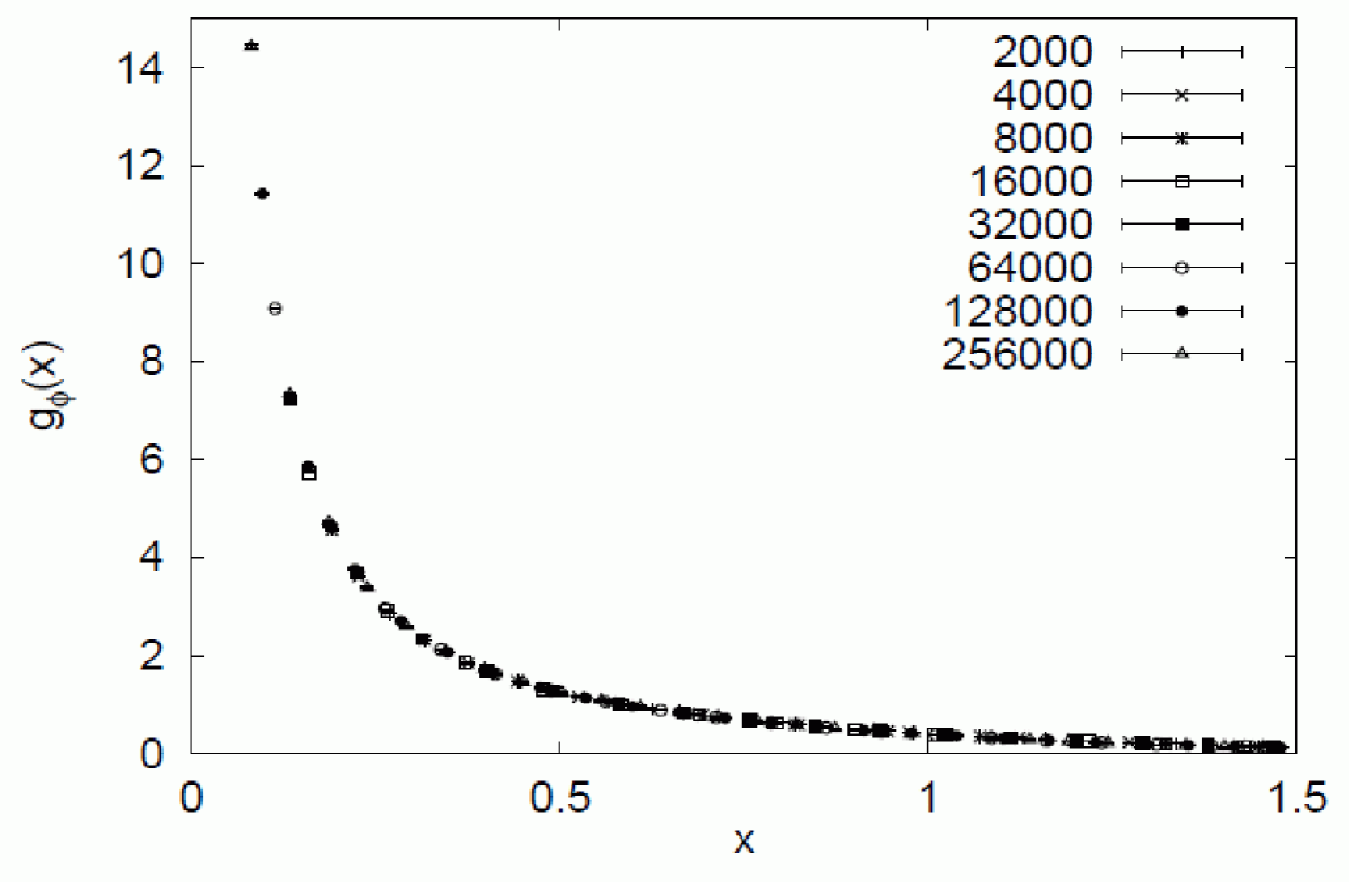
We note that eq. (62) has for form of a standard finite size scaling relation. One can thus apply the formula to the Ising model or 3-states Potts model and measure the spin-spin correlation functions for various values of $N$. Collapsing these correlation functions to universal functions $g_{\phi}(x)$ for either the Ising model ($c=1/2)$ or the 3-states Potts model $(c=4/5)$ allow us to determine both $d_{h}(c)$ and $\Delta(c)$ for these values of $c$. One finds a $d_{h}(c)$ in agreement with watabiki’s formula as mentioned earlier (but not with the same precision as with the method described in the last section), and one finds a $\Delta(c)$ in good agreement with the KPZ formula (59) [21]. The result of collapsing the data to a (best possible) universal function $g_{\phi}(x)$ is shown in Fig. 10 for the Ising model. It works very well for an impressive range of lattice sizes. Remarkably, finite size scaling works even better on the DT-ensemble of lattices than on a fixed lattice. Somehow the random lattices average out finite lattice artifacts.

Figure 16: The Ising spin correlation functions collapsed to the universal function $g_{\phi}(x)$ for the range of lattice sizes listed (measurements done for the Ising model at its annealed average critical point).

5 Conclusions

Two-dimensional quantum gravity is a nice playground for testing to what extent it makes sense to talk about non-trivial diffeomorphism invariant theories of fluctuating geometry. We have here focused on the very simplest question: if one integrates over the fluctuating geometries as one should do in a path integral representation of a quantum theory, how can one at all talk about concepts like distances and correlation functions falling off with this distance. In this context 2d quantum gravity is the perfect theory for such tests. It has no propagating gravitational degrees of freedom, but it is maximally quantum, the reason precisely being that the Einstein action in two dimensions is trivial. Every geometry carries therefore the same weight in the path integral, as exemplified by eq. (29), i.e. formally it corresponds to a $\hbar\to\infty$ limit. If we want to study ordinary field theories (like conformal field theories) and not just esoteric topological field theories, we cannot avoid the clash between the integration over all geometries and the need to have some concept of distance. However, as we have seen some aspects of geodesic distance remarkably survive this quantum average over geometries, despite the fact that geodesic distance is a awfully non-local notion. Although the geodesic distance picks up an anomalous dimension due to quantum fluctuations, it maintains its role as the distance which can be used in the correlators between fields.

In higher dimensions there might not exist a well-defined, stand-alone theory of quantum gravity. The UV problems for such a theory might be too severe. This question is still up in the air, and it might well be that the metric degrees of freedom we have in classical GR are not the fundamental degrees of freedom one should use in the UV regime. However, the studies reported here show that conceptually there seems to be no problem with a theory of “fluctuating” geometries per se and even in the most radical such one, namely 2d quantum gravity, one can maintain many of the concepts we know from flat spacetime.