Axion Dark Matter Detection using an LC Circuit

Abstract

It is shown that dark matter axions cause an oscillating electric current to flow along magnetic field lines. The oscillating current induced in a strong magnetic field $\vec{B}_{0}$ produces a small magnetic field $\vec{B}_{a}$. We propose to amplify and detect $\vec{B}_{a}$ using a cooled LC circuit and a very sensitive magnetometer. This appears to be a suitable approach to searching for axion dark matter in the $10^{-7}$ to $10^{-9}$ eV mass range.

Shortly after the Standard Model of elementary particles was established, the axion was postulated axion to explain why the strong interactions conserve the discrete symmetries P and CP. Further motivation for the existence of such a particle came from the realization that cold axions are abundantly produced during the QCD phase transition in the early universe and that they may constitute the dark matter axdm . Moreover, it has been claimed recently that axions are the dark matter, at least in part, CABEC ; case ; ban because axions form a Bose-Einstein condensate and this property explains the occurrence of caustic rings in galactic halos. The evidence for caustic rings with the properties predicted by axion BEC is summarized in ref. MWhalo . In supersymmetric extensions of the Standard Model, the dark matter may be a mixture of axions and supersymmetric dark matter candidates Baer .

Axion properties depend mainly on a single parameter $f_{a}$, called the axion decay constant. In particular the axion mass ($\hbar=c=1$)

$$m_{a}\simeq 6\cdot 10^{-6}~{}{\rm eV}~{}{10^{12}~{}{\rm GeV}\over f_{a}}$$ (1)

and its coupling to two photons

$${\cal L}_{a\gamma\gamma}=-g~{}a(x)\vec{E}(x)\cdot\vec{B}(x)$$ (2)

with $g=g_{\gamma}{\alpha\over\pi f_{a}}$. Here $a(x)$ is the axion field, $\vec{E}(x)$ and $\vec{B}(x)$ the electric and magnetic fields, $\alpha$ the fine structure constant, and $g_{\gamma}$ a model-dependent coefficient of order one. $g_{\gamma}\simeq-0.97$ in the KSVZ model KSVZ whereas $g_{\gamma}\simeq 0.36$ in the DFSZ model DFSZ . Cold axions are produced during the QCD phase transition, when the axion mass turns on and the axion field begins to oscillate in response. The resulting axion cosmological energy density is proportional to $(f_{a})^{7\over 6}$ and, in the simplest case, reaches the critical energy density for closing the universe when $f_{a}$ is of order 10¹² GeV axdm . This suggests that the most promising mass range in axion searches is near 10^-5 eV. This happens to be approximately where the cavity axion detection technique axdet is most feasible and where the ADMX experiment ADMX is searching at present.

However, it is desirable to search for axion dark matter over the widest possible mass range because the axion mass is, in reality, poorly constrained. In particular, it has been argued that if there is no inflation after the Peccei-Quinn phase transition, the contribution of axion strings to the axion cosmological energy density axcos implies that the preferred mass for dark matter axions is in the $10^{-3}$ to $10^{-4}$ eV mass range EPS . On the other hand, if there is inflation after the Peccei-Quinn phase transition, the axion field gets homogenized during inflation and the homogenized field may accidentally lie close to the minimum of its effective potential sypi , in which case axions may be the dark matter for masses much smaller than 10^-5 eV. String theory favors values of $f_{a}$ near the Planck scale and hence very small axion masses strax . It also predicts a variety of axion-like particles (ALPs) in addition to the axion that solves the strong CP problem Svrcek . For such ALPs there is no general relationship between the coupling $g$ to two photons and the mass $m_{a}$. ALPs produced by vacuum realignment are a form of cold dark matter with properties similar to axions Arias . The evidence for axion dark matter from axion Bose-Einstein condensation and the phenomenology of caustic rings does not depend sharply on the axion or ALP mass and therefore does not tell us anything precise about this parameter.

Other methods aside from the cavity technique have been proposed to search for dark matter axions. One proposed method consists of embedding an array of superconducting wires in a material transparent to microwave photons PDY . Dark matter axions convert to photons in the inhomogeneous magnetic field sourced by currents in the wires. This method appears best suited to searches for axions in the $10^{-4}$ eV mass range and above. Recent papers NMR propose the application of NMR techniques to axion detection. A sample of spin polarized material acquires a small oscillating transverse polarization as result of the axion dark matter background. The NMR techniques rely on the coupling of axions to nucleons. They are best suited to searches for axion dark matter with masses of order $10^{-8}$ eV and below. In addition to axion dark matter searches, there are searches for axions emitted by the Sun helio and ‘shining light through the wall’ experiments that attempt to produce and detect axions in the laboratory SLW . Stimulated by ref. NMR , we propose here a new method to search for dark matter axions. It exploits the coupling of the axion to two photons and appears suitable to axion dark matter searches in the $10^{-7}$ eV range and below. Using a combination of the various approaches it may be possible to search for dark matter axions over a wide mass range, from approximately $10^{-9}$ to $10^{-4}$ eV.

The coupling of the axion to two photons, Eq. (2), implies that the inhomogenous Maxwell equations are modified axdet as follows:

$$\vec{\nabla}\cdot\vec{E} = g\vec{B}\cdot\vec{\nabla}a+\rho_{\rm el}$$

$$\vec{\nabla}\times\vec{B}-{\partial\vec{E}\over\partial t} = g(\vec{E}\times\vec{\nabla}a-\vec{B}{\partial a\over\partial t})+\vec{j}_{\rm el}$$ (3)

where $\rho_{\rm el}$ and $\vec{j}_{\rm el}$ are electric charge and current densities associated with ordinary matter. Eq.  (3) shows that, in the presence of an externally applied magnetic field $\vec{B}_{0}$, dark matter axions produce an electric current density $\vec{j}_{a}=-g\vec{B}_{0}\dot{a}$, where $\dot{a}\equiv{\partial a\over\partial t}$. Assuming the magnetic field to be static, $\vec{j}_{a}$ oscillates with frequency

$$\omega=m_{a}(1+{1\over 2}\vec{v}\cdot\vec{v})$$ (4)

where $\vec{v}$ is the axion velocity. Let us assume that the spatial extent of the externally applied magnetic field is much less than $m_{a}^{-1}$. $\vec{j}_{a}$ produces then a magnetic field $\vec{B}_{a}$ such that $\vec{\nabla}\times\vec{B}_{a}=\vec{j}_{a}$. Our proposal is to amplify $\vec{B}_{a}$ using an LC circuit and detect the amplified field using a SQUID or SERF magnetometer.

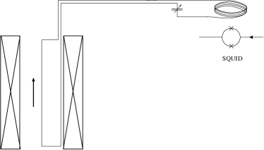
Figure 1: Schematic drawing of the proposed axion dark matter detector, in the case where the magnet is a solenoid. The two crossed rectangles indicate cross-sections of the solenoid’s windings. The direction of the magnetic field ($\vec{B}_{0}$) produced by the solenoid is indicated by an arrow.

Fig. 1 shows a schematic drawing in case the magnet producing $\vec{B}_{0}$ is a solenoid. The field $\vec{B}_{a}$ has flux $\Phi_{a}$ through a LC circuit, made of superconducting wire. Because the wire is superconducting, the total magnetic flux through the circuit is constant. In the limit where the capacitance of the LC circuit is infinite (or the capacitor is removed), the current in the wire is $I=-\Phi_{a}/L$ where $L$ is the inductance of the circuit in its environment, i.e. including the effect of mutual inductances with neighboring circuits. The magnetic field seen by the magnetometer is ($\mu_{0}$ = 1)

$$B_{d}\simeq{N_{d}\over 2r_{d}}I=-{N_{d}\over 2r_{d}~{}L}\Phi_{a}$$ (5)

where $N_{d}$ is the number of turns and $r_{d}$ the radius of the small coil facing the magnetometer. Ignoring for the moment mutual inductances with neighboring circuits, $L$ is a sum

$$L\simeq L_{m}+L_{c}+L_{d}$$ (6)

of contributions $L_{m}$ from the large pickup loop inside the externally applied magnetic field, $L_{d}$ from the small coil facing the magnetometer, and $L_{c}$ from the co-axial cable in between. We have

$$L_{d}=r_{d}N_{d}^{2}c_{d}$$ (7)

with

$$c_{d}\simeq\ln\left({8r_{d}\over a_{d}}\right)-2$$ (8)

where $a_{d}$ is the radius of the wire in the small coil. If mutual inductances are important, their effect upon $L$ must be included and Eq (6) modified. For example, if there is a single neighboring circuit with self-inductance $L_{22}$ and mutual inductance $L_{12}$ with the LC circuit, and if $\vec{B}_{a}$ has no flux through this second circuit, then

$$L\simeq L_{m}+L_{c}+L_{d}-(L_{12})^{2}/L_{22}~{}~{}~{}\ .$$ (9)

We note that the currents in the coil sourcing the $\vec{B}_{0}$ field are generally perpendicular to the currents flowing in the pickup loop, so that the mutual inductance between the coil and pickup loop is suppressed. Also, when Eq. (9) is valid, $L$ is smaller than in the $L_{12}=0$ case, and hence $B_{d}$ is increased. When discussing the LC circuit’s optimization and estimating the detector’s sensitivity below, we will ignore mutual inductances. Mutual inductances should be measured in any actual setup and the optimization and sensitivity estimates adjusted accordingly.

For finite $C$, the LC circuit resonates at frequency $\omega=1/\sqrt{LC}$. When $\omega$ equals the axion rest mass, the magnitude of the current in the wire is multiplied by the quality factor $Q$ of the circuit and hence

$$B_{d}\simeq{QN_{d}\Phi_{a}\over 2Lr_{d}}~{}~{}~{}\ .$$ (10)

We expect that a quality factor $Q$ of order $10^{4}$ may be achieved by using high $T_{c}$ superconducting wire for the part of the LC circuit in the high magnetic field region HTC and by placing superconducting sleeves between the LC circuit and nearby ordinary metals.

Let us consider the case where the externally applied magnetic field is homogeneous, $\vec{B}_{0}=B_{0}\hat{z}$, as is approximately true inside a long solenoid. In such a region

$$\vec{B}_{a}=-{1\over 2}g\dot{a}B_{0}\rho\hat{\phi}$$ (11)

where ($z$, $\rho$, $\phi$) are cylindrical coordinates and $\hat{\phi}$ is the unit vector in the direction of increasing $\phi$. For the pickup loop depicted in Fig. 1, a rectangle whose sides $l_{m}$ and $r_{m}$ are approximately the length and radius of the magnet bore, the flux of $\vec{B}_{a}$ through the pickup loop is

$$\Phi_{a}=-V_{m}g\dot{a}B_{0}$$ (12)

with $V_{m}={1\over 4}l_{m}r_{m}^{2}$. The self-inductance of the pickup loop is $L_{m}\simeq{1\over\pi}l_{m}\ln\left({r_{m}\over a_{m}}\right)$ where $a_{m}$ is the radius of the wire. We may also consider the case $\vec{B}_{0}=B_{0}(\rho)\hat{\phi}$, as is approximately true in a toroidal magnet. Here one introduces a circular pickup loop at $\rho=R_{m}$. We have then Eq. (12) with

$$V_{m}B_{0}=2\pi\int_{0}^{R_{m}}\rho~{}d\rho~{}\int_{\rho}^{\infty}d\rho^{\prime}B_{0}(\rho^{\prime})$$ (13)

and $L_{m}\simeq R_{m}[\ln\left({8R_{m}\over a_{m}}\right)-2]$.

The time derivative of the axion field is related to the axion density by $\rho_{a}={1\over 2}\dot{a}^{2}$. Hence, combining Eqs. (10) and (12), we have

$$B_{d} \simeq {N_{d}Q\over 2r_{d}L}V_{m}g\sqrt{2\rho_{a}}B_{0}=1.25\cdot 10^{-15}~{}{\rm T}\cdot$$ (14)

$$\cdot \left({\rho_{a}\over{\rm GeV/cm}^{3}}\right)^{1\over 2}\left({Q\over 10^{4}}\right)\left({g\over 10^{-17}{\rm GeV}^{-1}}\right)\cdot$$

$$\cdot N_{d}\left({{\rm cm}\over r_{d}}\right)\left({V_{m}\over{\rm m}^{3}}\right)\left({\mu{\rm H}\over L}\right)\left({B_{0}\over 10~{}{\rm T}}\right)\ .$$

In comparison the sensitivity of today’s best magnetometers is $\delta B=B_{n}\sqrt{\Delta\nu\over{\rm Hz}}$ with $B_{n}$ of order $10^{-16}~{}{\rm T}$. A quality factor of $10^{4}$ implies that the detector bandwidth is $10^{-4}\nu$. If a factor 2 in frequency is to be covered per year, and the duty factor is 30%, the amount of time spent at each tune of the LC circuit is of order $10^{3}$ seconds.

The signal to noise ratio will depend on the signal coherence time which in turn depends on the velocity dispersion of the axions. We consider two different assumptions for the local axion velocity distribution. Assumption A is that the isothermal halo model is correct MST . In that case the local dark matter density is of order $\rho_{\rm dm}\simeq 300$ MeV/${\rm cm}^{3}$ and the velocity dispersion is of order $\delta v\simeq 10^{-3}$. The energy dispersion is of order $\delta E\simeq 10^{-6}m_{a}$ and hence the coherence time $t_{c}=1/\delta E\simeq 0.16~{}{\rm s}({\rm MHz}/\nu)$ where $\nu$ is the frequency associated with the axion mass: $m_{a}=2\pi\nu$. Under assumption A, the magnetometer can detect a magnetic field $B_{d}=10^{-16}~{}{\rm T}~{}({\rm Hz})^{-{1\over 2}}~{}(t_{c}~{}t)^{-{1\over 4}}\simeq 2.8\cdot 10^{-17}~{}{\rm T}\left({\nu\over{\rm MHz}}\right)^{1\over 4}$ in $t=10^{3}$ s of integration time. Assumption B is that the caustic ring halo model is correct MWhalo . In that case the local dark matter distribution is dominated by a single flow with density $\rho_{\rm dm}\simeq$ 1 GeV/${\rm cm}^{3}$, velocity $v\simeq$ 309 km/s and velocity dispersion $\delta v\lesssim$ 53 m/s. The energy dispersion of that flow $\delta E=m_{a}v\delta v\lesssim 1.8\cdot 10^{-10}m_{a}$ and hence $t_{c}\gtrsim 880~{}{\rm s}({\rm MHz}/\nu)$. However, the Earth’s rotation continually shifts the flow velocity in the laboratory by an amount of order 2 cm/s per second. If this Doppler shift is not removed, there is an upper limit on the coherence time of order $t_{c}<1.4\cdot 10^{3}~{}{\rm s}({\rm MHz}/\nu)^{1\over 2}$. The Doppler shift can be partially removed by exploiting information about the velocity vector of the locally dominant flow MWcr . Under assumption B, we expect therefore the signal to be coherent over the whole $10^{3}$ seconds of measurement integration time and hence the magnetometer sensivity to be of order $3.2\cdot 10^{-18}$ T. Under assumption B, the signal to noise ratio is approximately a factor 15 larger than under assumption A, a factor 9 because of the increased coherence time and a factor 1.7 because of the increased density. Recently, the caustic ring model has been modified ban . In the modified model, the densities of all local flows are increased by a factor of order five. The signal to noise ratio is then increased by a factor of order 2.2 compared to assumption B.

We now consider other sources of noise, in addition to the noise in the magnetometer. Most importantly, there is thermal (Johnson-Nyquist) noise in the LC circuit. It causes voltage fluctuations $~{}\delta V_{T}=\sqrt{4k_{B}T~{}R~{}\Delta\nu}~{}$ nyq and hence current fluctuations

$$\delta I_{T}={\delta V_{T}\over R}=\sqrt{4k_{B}TQ\Delta\nu\over L\omega}=2.96\cdot 10^{-13}{\rm A}\cdot$$ (15)

$$\cdot \sqrt{\left({{\rm MHz}\over\nu}\right)\left({\mu{\rm H}\over L}\right)\left({Q\over 10^{4}}\right)\left({T\over{\rm mK}}\right)\left({\Delta\nu\over{\rm mHz}}\right)}$$

where we used the relation $R={L\omega\over Q}$ between the resistance and quality factor of a LC circuit. We expect that it will be possible to cool the LC circuit to below 0.5 ${\rm mK}$ in two stages, using a dilution refrigerator followed by a nuclear demagnetization refrigerator. A temperature of 0.4 ${\rm mK}$ was achieved at the NHMFL Ultra-High B/T Facility using this technique Sull . Eq. (15) should be compared with the current due to the signal

$$I = {Q\over L}V_{m}g\dot{a}B_{0}=1.99\cdot 10^{-11}{\rm A}\left({Q\over 10^{4}}\right)\left({\mu{\rm H}\over L}\right)\left({V_{m}\over{\rm m}^{3}}\right)\cdot$$ (16)

$$\cdot \left({g\over 10^{-17}{\rm GeV}^{-1}}\right)\sqrt{\rho_{a}\over{\rm GeV}/{\rm cm}^{3}}\left({B_{0}\over 10~{}{\rm T}}\right)$$

and with the fluctuations in the measured current due to the noise in the magnetometer

$$\delta I_{B} \simeq {2r_{d}\over N_{d}}\delta B=5.03\cdot 10^{-14}{\rm A}\cdot$$ (17)

$$\cdot {1\over N_{d}}\left({r_{d}\over{\rm cm}}\right)\left({B_{n}\over 10^{-16}~{}{\rm T}}\right)\sqrt{\Delta\nu\over{\rm mHz}}\ .$$

Another possible source of noise is flux jumps in the magnet that produces the $\vec{B}_{0}$ field. Such flux jumps are caused by small sudden displacements in the positions of the wires in the magnet windings. Since the jumps occur over time scales of order $10^{-2}$ to $10^{-3}$ s, the noise they produce at MHz frequencies is suppressed. Such flux jumps are a negligble source of noise in ADMX, which however operates at GHz frequencies. This noise would also affect the proposals of ref. NMR . Finally, there are false signals associated with man-made electromagnetic radiation. Such false signals are commonly seen in ADMX but can easily be eliminated by various tests. They can be avoided altogether by placing the detector in a Faraday cage but, as with ADMX, this may not be necessary.

Assuming that thermal and magnetometer noise are the main backgrounds, the signal to noise ratio is

$$s/n={I\over\sqrt{(\delta_{T}I)^{2}+(\delta_{B}I)^{2}}}$$ (18)

with $I$, $\delta I_{T}$ and $\delta I_{B}$ given above, and $L$ given by Eqs. (6) and (7). The $s/n$ ratio may be optimized with respect to $N_{d}$ and $r_{d}$. It is best to make $r_{d}$ as small as conveniently possible. The optimal value of $N_{d}$ is

$$N_{d}=\sqrt{{L\over L_{e}}\left(\sqrt{1+{L_{e}\over c_{d}r_{d}}}-1\right)}$$ (19)

with

$$L_{e} = {k_{B}TQ{\rm Hz}\over r_{d}^{2}B_{n}^{2}\omega}=35\mu{\rm H}\left({{\rm cm}\over r_{d}}\right)^{2}\left({{\rm MHz}\over\nu}\right)\left({Q\over 10^{4}}\right)\cdot$$ (20)

$$\cdot \left({T\over{\rm mK}}\right)\left({10^{-16}~{}{\rm T}\over B_{n}}\right)^{2}\ .$$

For the experimental parameters envisaged, the magnetometer noise is always much less than the thermal noise.

Fig. II shows the limits that can be placed on $g$ using two specific magnets. In each case, the limits make assumption B for the local axion velocity distribution ($t=t_{c}=10^{3}$ s). Furthermore we assumed $Q=10^{4}$, $T=0.5$ mK, and that all axion candidate signals with $s/n>5$ have been ruled out. The two magnets are: a) the ADMX magnet ($l_{m}$ = 1 m, $r_{m}$ = 0.3 m, $L_{m}$ = 2.4 $\mu$H, $L_{c}$ = 0.2 $\mu$H, $B_{0}$ = 8 T), b) the CMS magnet ($l_{m}$ = 13 m, $r_{m}$ = 3 m, $L_{m}$ = 37 $\mu$H, $L_{c}$ = 0.5 $\mu$H, $B_{0}$ = 4 T). Because of stray capacitance each LC circuit has a maximum frequency. We calculated the cutoff frequencies assuming that the stray capacitance is 15 pF per meter of circuit length. As discussed above, under assumption A for the local axion density and velocity distribution, the expected limits are approximately a factor 15 weaker than shown in Fig. II.

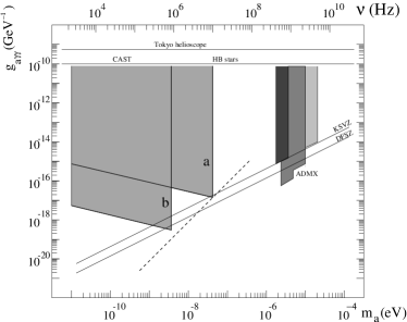
Figure 2: Expected senstivity of the proposed detector. The horizontal lines near the top indicate upper limits on $g$ from stellar evolution (horizontal branch stars) and from the Tokyo and CAST solar axion searches helio . The shaded areas on the right are limits obtained (dark) and anticipated (lighter) by the ADMX axion dark matter search. The light shaded areas on the left show the expected sensitivity of the proposed experiment, under the assumptions spelled out in the text, using a) the ADMX magnet, and b) the CMS magnet. The dashed line indicates how the sensitivity scales with the magnet’s physical size, keeping everything else fixed.

We are grateful to John Clarke for useful comments. This work was supported in part by the U.S. Department of Energy under contract DE-FG02-97ER41029.

References

- (1) R. D. Peccei and H. Quinn, Phys. Rev. Lett. 38 (1977) 1440 and Phys. Rev. D16 (1977) 1791; S. Weinberg, Phys. Rev. Lett. 40 (1978) 223; F. Wilczek, Phys. Rev. Lett. 40 (1978) 279.
- (2) J. Preskill, M. Wise and F. Wilczek, Phys. Lett. B120 (1983) 127; L. Abbott and P. Sikivie, Phys. Lett. B120 (1983) 133; M. Dine and W. Fischler, Phys. Lett. B120 (1983) 137.
- (3) P. Sikivie and Q. Yang, Phys. Rev. Lett. 103 (2009) 111301.
- (4) P. Sikivie, Phys. Lett. B695 (2011) 22.
- (5) N. Banik and P. Sikivie, arXiv:1307.3547.
- (6) L.D. Duffy and P. Sikivie, Phys. Rev. D78 (2008) 063508.
- (7) H. Baer, arXiv:1310.1859, and references therein.
- (8) J. Kim, Phys. Rev. Lett. 43 (1979) 103; M. A. Shifman, A. I. Vainshtein and V. I. Zakharov, Nucl. Phys. B166 (1980) 493.
- (9) A. P. Zhitnitskii, Sov. J. Nucl. 31 (1980) 260; M. Dine, W. Fischler and M. Srednicki, Phys. Lett. B104 (1981) 199.
- (10) P. Sikivie, Phys. Rev. Lett. 51 (1983) 1415 and Phys. Rev. D32 (1985) 2988.
- (11) S. Asztalos et al., Phys. Rev. Lett. 104 (2010) 041301 and references therein.
- (12) For a review see: P. Sikivie, Lect. Notes Phys. 741 (2008) 19.
- (13) M. Yamaguchi, M. Kawasaki and J. Yokoyama, Phys. Rev. Lett. 82 (1999) 4578; O. Wantz and E.P.S. Shellard, Phys. Rev. D82 (2010) 123508.
- (14) S.-Y. Pi, Phys. Rev. Lett. 52 (1984) 1725.
- (15) E. Witten, Phys. Lett. B149 (1984) 351; K. Choi and J.E. Kim, Phys. Lett. B154 (1985) 393.
- (16) P. Svrcek and E. Witten, JHEP 0606 (2006) 051; A. Arvanitaki et al., Phys. Rev. D81 (2010) 123530.
- (17) P. Arias et al., JCAP 1206 (2012) 013.
- (18) P. Sikivie, D.B. Tanner and Y. Wang, Phys. Rev. D50 (1994) 4744.
- (19) P. Graham and S. Rajendran, Phys. Rev. D88 (2013) 035023; D. Budker et al., arXiv:1306.6089.
- (20) Y. Inoue et al., Phys. Lett. B668 (2008) 93; E. Arik et al., JCAP 0902 (2009) 008, and references therein.
- (21) K. Ehret et al., Phys. Lett. B689 (2010) 149, and references therein.
- (22) R.D. Black, T.A. Early and G.A. Johnson, J. of Magn. Res. A113 (1995) 74; S.M. Anlage, in Microwave Superconductivity, Kluwer Academic Publ. 2001, p 337-352, and references therein.
- (23) M.S. Turner, Phys. Rev. D33 (1986) 889.
- (24) P. Sikivie, Phys. Lett. B567 (2003) 1.
- (25) H. Nyquist, Phys. Rev. 32 (1928) 110.
- (26) N.S. Sullivan et al., Physica B 294-295 (2001) 519.