Numerical Stochastic Perturbation Theory in the Schrödinger Functional

Abstract:

The Schrödinger functional (SF) is a powerful and widely used tool for the treatment of a variety of problems in renormalization and related areas. Albeit offering many conceptual advantages, one major downside of the SF scheme is the fact that perturbative calculations quickly become cumbersome with the inclusion of higher orders in the gauge coupling and hence the use of an automated perturbation theory framework is desirable. We present the implementation of the SF in numerical stochastic perturbation theory (NSPT) and compare first results for the running coupling at two loops in pure $SU(3)$ Yang-Mills theory with the literature.

1 Numerical Stochastic Perturbation Theory and the Schrödinger Functional

We consider the Schödinger functional as defined in [1]. Specifically, the $SU(3)$ gauge field variables $U_{\mu}(x)$ are subject to periodic boundary conditions in the spatial directions and Dirichlet ones in the temporal directions,

$$U_{k}(x)|_{x_{0}=0}=e^{aC_{k}}\,,\quad U_{k}(x)|_{x_{0}=T}=e^{aC_{k}^{\prime}}\,.$$ (1)

The presence of Dirichlet boundary conditions induces a background field as was discussed at length in [1], which can be exploited for a number of interesting applications, most prominently for the determination of the running gauge coupling as we will shortly review. The most common choices of the matrices $C_{k},C_{k}^{\prime}$ are either zero, in which case we will speak of a trivial background field, and constant diagonal matrices as specified in [2], which gives raise to an Abelian background field,

$$V_{\mu}(x)=e^{aB_{\mu}(x)}\,,\quad B_{0}=0\,,\quad B_{k}=\left[x_{0}C_{k}^{\prime}+(T-x_{0})C_{k}\right]/L\,.$$ (2)

Close to the classical minimum, the gauge fields may then be written as

$$U_{\mu}(x)=e^{a\,g_{0}\,q_{\mu}(x)}V_{\mu}(x)\,.$$ (3)

The gauge action is given by

$$S[U]=\frac{1}{g_{0}^{2}}\sum_{p}w(p)\operatorname{tr}\left\{1-U(p)\right\}\,,$$ (4)

where we sum over all oriented plaquettes $p$, $U(p)$ is the closed parallel transporter around $p$, and the weight factor is unity everywhere on the lattice except for the plaquettes that contain a frozen spatial link at the boundary (1) and a temporal link, for which we set

$$w(p)|_{\rm boundary}=c_{t}=1+g_{0}^{2}c_{t}^{(1)}+g_{0}^{4}c_{t}^{(2)}+\ldots\,,$$ (5)

with $c_{t}^{(1)}=-0.08896(23)$ as quoted in [3]. This ensures cancellation of $O(a)$ cut-off effects introduced by the boundary.

Numerical stochastic perturbation theory is reviewed in detail in [4]. It is a numerical implementation of stochastic perturbation theory, which solves the equations of stochastic quantization order by order in the coupling constant of the theory. Specifically, one introduces a new degree of freedom, the stochastic time $t$ and considers solutions of the Langevin equation,

$$\partial_{t}U^{\eta}_{\mu}(x;t)=\left\{-i\,\nabla_{x\mu}S[U]-i\eta_{x\mu}(t)\right\}U^{\eta}_{\mu}(x;t)\,,$$ (6)

where the gauge field now acquires a formal dependence on the choice of the Gaussian noise variables $\eta(t)=T^{a}\eta^{a}$, which in turn satisfy

$$\big{\langle}\eta^{a}_{x\mu}(t)\big{\rangle}_{\eta} =0\,, \big{\langle}\eta^{a}_{x\mu}(t)\eta^{b}_{y\nu}(t^{\prime})\big{\rangle}_{\eta} =2\,\delta^{ab}\delta_{xy}\delta_{\mu\nu}\delta(t-t^{\prime})\,.$$ (7)

The main assertion of stochastic quantization ([5, 6]) is that the noise average of any (in the case at hand, gauge-invariant) observable $O(U)$ converges, in the limit of large stochastic time, to the usual path integral average

$$\big{\langle}O(U_{\mu}^{\eta})\big{\rangle}_{\eta}\xrightarrow{t\to\infty}\big{\langle}O\big{\rangle}\,.$$ (8)

In particular in the case of non-Abelian gauge theories the proof of (1.8) is non-trivial, but it is rigorous in perturbation theory [7]. Hence the solution to the Langevin equation may be consistently expanded in the coupling constant

$$U_{\mu}(x)=V_{\mu}(x)+\sum_{i=1}^{N}g_{0}^{i}\,U_{\mu}^{(i)}(x)+O\left(g_{0}^{N+1}\right)\,.$$ (9)

NSPT amounts to storing the perturbative expansion of the gauge field on a computer and numerically solving the order-by-order version of the Langevin equation. This is done using e.g. an Euler or Runge-Kutta integrator. During integration, all multiplications of gauge fields (9) have to be performed order-by-order, which may be conveniently implemented using any modern object-oriented programming language. We choose to employ the second-order Runge-Kutta method described in [8], introducing discretization errors proportional to the squared integration step-size $\tau^{2}$. These cut-off effects have to be extrapolated to zero in the final analysis. The form of the expansion (9) makes it clear that trivial as well as Abelian background fields may be accommodated. A more detailed description of our implementation may be found in [9].

1.1 Stochastic Gauge Fixing

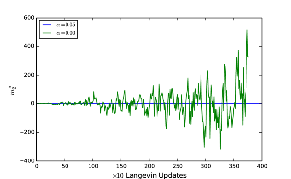
Figure 1: The effect of stochastic gauge fixing.

Zwanziger described in [10] a method to perform gauge fixing in a theory that has been quantized stochastically. As explained in [4], a similar approach, which we want to call gauge suppression here, is crucial to extract results form NSPT. The noise term in the Langevin equation (6) drives all modes of the gauge field, while only the transversal ones are then damped by the term proportional to the group derivative of the gauge action. The longitudinal modes, even though they do not contribute to expectation values of gauge-invariant quantities, need to be damped as well if one hopes to extract numerical results, which are otherwise drowned out in noise. To construct a gauge transformation which will damp the unwanted modes with SF boundary conditions present, we proceed in the usual fashion (see e.g. [11] for a review) by finding a suitable functional $W[U]$ whose extremal value is characterized by the gauge fixing condition (as specified in [1]) being fulfilled. Our choice is given by

$$W[U]=-\,a^{2}\sum_{(x,\mu)\in\Lambda}\cosh\{ag_{0}q_{\mu}(x)\}\,,$$ (10)

where $\Lambda$ is the set of all indices belonging to dynamical links. The functional (10) is driven to its stationary point by applying gauge fixing transformations $\Omega(x)=e^{-i\,\epsilon\,\omega(x)}$ with, in the case of an Abelian background field,

$$\omega(x)=\begin{cases}-\alpha\sum_{\mu}\left.D_{\mu}^{*}\sinh\{ag_{0}q_{\mu}(x)\}\right|_{\rm traceless}\,,&{\rm if~{}}\,0<x_{0}<T\,,\\ -\alpha\left(\frac{a}{L}\right)^{3}\sum_{x,x_{0}=0}\left.\sinh\{ag_{0}q_{0}(x)\}_{jj}\right|_{\rm traceless}\,,&{\rm if~{}}\,x_{0}=0\\ 0&{\rm else}\,,\end{cases}$$ (11)

with $0<\alpha<1$, $j$ being a color index (i.e. we refer to the diagonal, traceless part in the second line of (11)), and the covariant derivative as specified in [1]. In the case of a trivial background field, one has to consider the full color matrix at $x_{0}=0$. To demonstrate the high sensitivity of NSPT simulations on the gauge suppression being in place, we performed two runs, starting from the same thermalized configuration on a $L/a=4$ lattice with integration step size $\tau=0.02$, one with gauge suppression in place and another one with $\alpha=0$. The effect is rather dramatic, even tough the mean value remains the same, the errors explode due to ever-growing fluctuations, as seen in figure 1. The observable considered there will be introduced in the following section.

2 The Gauge Coupling

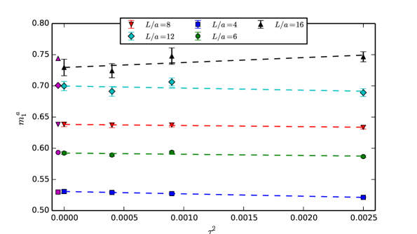
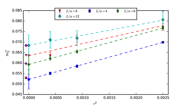
Figure 2: Results for $m_{1}^{a}$ and $m_{2}^{a}$, the magenta points represent the known results.

As a suitable test case to reliably check the correctness of our implementation, we chose to re-calculate the two-loop results of the Schrödinger functional coupling presented in [3]. The boundary values for the gauge fields chosen in [2] depend on a parameter $\eta$, which may be used to define a running coupling $\overline{g}$ using the free energy

$$e^{-\Gamma}=\int D{U}e^{-S[U]}\,,$$ (12)

by setting

$$\overline{g}^{2}=k/\partial_{\eta}\Gamma=g_{0}^{2}+m_{1}\,g_{0}^{4}+m_{2}\,g_{0}^{6}+\ldots\,,$$ (13)

where the constant $k$ ensures correct normalization. As in [3], we will adapt a notation to single out the contributions coming from the weight factor (5), writing

$$m_{1}=\; m_{1}^{a}+c_{t}^{(1)}\,m_{1}^{b}\,,$$ (14)

$$m_{2}-m_{1}^{2}=\; m_{2}^{a}+c_{t}^{(1)}\,m_{2}^{b}+\left(c_{t}^{(1)}\right)^{2}\,m_{2}^{c}+c_{t}^{(2)}\,m_{2}^{d}\,.$$ (15)

All individual parts of (14) and (15) were calculated in [3] for a range of lattice resolutions $L/a$. First, we neglect the effect of boundary improvement and set $c_{t}=1$, focusing on reproducing $m_{1}^{a}$ and $m_{2}^{a}$. We performed a number of exploratory simulations on rather small lattices with $L/a$ ranging from four to 16. We did not find it worthwhile to push the lattice sizes further since our main aim is to prove the correctness of our implementation of the Schrödinger functional in NSPT. To do so, we proceed as follows. For each chosen lattice size $L/a$, we performed three simulations varying the integration step size $\tau\in\{0.02,0.03,0.05\}$. We estimated the mean value and variance by taking into account the integrated autocorrelation time, estimated as recommended in [12]. We then extrapolated $\tau\to 0$ using both a linear fit to all data points and a constant fit to the data omitting $\tau=0.05$. The difference in the fits is then added to the statistical error as an estimate for systematic effects in the extrapolation, giving the NSPT estimate $m_{i}^{a,\rm NSPT}$ and error $\delta m_{i}^{a,\rm NSPT}$. The results for $m_{1}^{a}$ and $m_{2}^{a}$ may be found in figure 2. We define the precision of our estimate by comparing with the known results,

$$\Delta m_{i}^{a}=\left|m_{i}^{a}-m_{i}^{a,\rm NSPT}\right|\,.$$ (16)

$L/a$		4		6		8		12		16
$\tau$		0.02	0.03	0.02	0.03	0.02	0.03	0.02	0.03	0.02	0.03
$g_{0}^{2}$	$N_{\rm eff}$	11466	16760	5851	8242	2256	3804	864	1363	478	353
	$\tau_{\rm int}$	12.6(4)	8.6(2)	41(2)	29(1)	66(4)	39(2)	83(8)	53(4)	92.9(1)	62(8)
	$\Delta m_{1}^{a}$	0.0009(27)		0.0010(21)		0.0000(37)		0.0009(74)		0.014(13)
$g_{0}^{4}$	$N_{\rm eff}$	12489	17334	6105	8545	2544	3633	825	1181	327	221
	$\tau_{\rm int}$	11.5(3)	8.3(2)	39(2)	27.9(10)	59(3)	41(2)	87(8)	61(5)	135.9(2)	99.2(2)
	$\Delta m_{2}^{a}$	0.0007(46)		0.0004(46)		0.0002(44)		0.0001(49)		0.0032(88)

Table 1: Details of simulations performed.

The details of our simulations are summarized in table 1, where we omitted the data points at the biggest integration step size for space reasons (the performance is anyway limited by the simulation with smallest step size due to larger autocorrelation times). In addition to the integrated autocorrelation time in units of Langevin integration steps and precision of our estimation, we state the effective number of measurements $N_{\rm eff}=N_{\rm updates}/(2\tau_{\rm int})$. The total run-time for $L/a=12$, leading to a result of $m_{2}^{a}=0.0684(49)$ was 210h on a single node of the Lonsdale cluster at Trinity College (AMP Opteron, 8 cores/node).

2.1 Boundary Improvement

$L/a$		4			6			8
$\tau$		0.02	0.032	0.04	0.02	0.032	0.04	0.02	0.032	0.04
$g_{0}^{2}$	$N_{\rm eff}$	6418	6357	6225	2775	3069	2776	1286	1266	1193
	$\tau_{\rm int}$	13.3(5)	7.8(3)	6.7(3)	21(1)	13.0(7)	10.7(6)	28(2)	16(1)	15(1)
	$\Delta m_{1}$	0.0026(64)			0.0007(27)			0.0030(39)

Table 2: Details of simulations performed including $c_{t}^{(1)}$.

For many applications, boundary improvement is a necessity. Hence we performed a few additional simulations, now including $c_{t}^{(1)}$ in the gauge update step. Note that up to $O(g_{0}^{6})$ this is sufficient to capture all non-tree-level dynamic, as the contribution involving $c_{t}^{(2)}$ multiplies a tree-level counter-term. The results are presented in table 2 and are found to be in complete agreement with what was found in [3]. We did not attempt to extract $m_{2}$ due to limited statistics.

3 Conclusions

The availability of the Schrödinger functional in NSPT opens the door to a variety of interesting applications, in particular connected to the Wilson flow method [13], as will be further discussed in [14]. We are confident in the correctness and performance of our code, using trivial as well as Abelian background fields. The inclusion of dynamical fermions is well on the way.

Acknowledgements

We would like to thank the teams of the computing center at Trinity College (TCHPC) and the Irish Centre for High End Computing (ICHEC) for their support in performing the numerical simulations. S. Sint acknowledges support by SFI under grant 11/RFP/PHY3218. M. Dalla Brida is supported by the Irish Research Council. This work received funding from the Research Executive Agency (REA) of the European Union under Grant Agreement number PITN-GA-2009-238353 (ITN STRONGnet) and in parts by INFN under i.s. MI11 (now QCDLAT).

References

- [1] Martin Lüscher, Rajamani Narayanan, Peter Weisz, and Ulli Wolff. The Schrödinger functional: A Renormalizable probe for nonAbelian gauge theories. Nucl.Phys., B384:168–228, 1992.
- [2] Martin Lüscher, Rainer Sommer, Peter Weisz, and Ulli Wolff. A Precise determination of the running coupling in the SU(3) Yang-Mills theory. Nucl.Phys., B413:481–502, 1994.
- [3] Achim Bode, Ulli Wolff, and Peter Weisz. Two loop computation of the Schrödinger functional in pure SU(3) lattice gauge theory. Nucl.Phys., B540:491–499, 1999.
- [4] F. Di Renzo and L. Scorzato. Numerical stochastic perturbation theory for full QCD. JHEP, 0410:073, 2004.
- [5] Poul H. Damgaard and Helmuth Huffel. Stochastic Quantization. Phys.Rept., 152:227, 1987.
- [6] G. Parisi and Yong-shi Wu. Perturbation Theory Without Gauge Fixing. Sci.Sin., 24:483, 1981.
- [7] E. Floratos and J. Iliopoulos. Equivalence of Stochastic and Canonical Quantization in Perturbation Theory. Nucl.Phys., B214:392, 1983.
- [8] C. Davies, G. Batrouni, G. Katz, P. Lepage, P. Rossi, et al. Langevin simulations of lattice field theories using Fourier acceleration. J.Statist.Phys., 43:1073–1075, 1986.
- [9] Michele Brambilla, Dirk Hesse, and Francesco Di Renzo. Code development (not only) for NSPT. PoS, LATTICE2013:418, 2013.
- [10] Daniel Zwanziger. Covariant Quantization of Gauge Fields Without Gribov Ambiguity. Nucl.Phys., B192:259, 1981.
- [11] Leonardo Giusti, M.L. Paciello, C. Parrinello, S. Petrarca, and B. Taglienti. Problems on lattice gauge fixing. Int.J.Mod.Phys., A16:3487–3534, 2001.
- [12] Ulli Wolff. Monte Carlo errors with less errors. Comput.Phys.Commun., 156:143–153, 2004.
- [13] Martin Lüscher. Properties and uses of the Wilson flow in lattice QCD. JHEP, 1008:071, 2010.
- [14] Mattia Dalla Brida and Dirk Hesse. Numerical Stochastic Perturbation Theory and the Gradient Flow. PoS, LATTICE2013:326, 2013.