Hybridized discontinuous Galerkin method for convection-diffusion problems

Abstract

In this paper, we propose a new hybridized discontinuous Galerkin (DG) method for the convection-diffusion problems with mixed boundary conditions. A feature of the proposed method, is that it can greatly reduce the number of globally-coupled degrees of freedom, compared with the classical DG methods. The coercivity of a convective part is achieved by adding an upwinding term. We give error estimates of optimal order in the piecewise $H^{1}$-norm for general convection-diffusion problems. Furthermore, we prove that the approximate solution given by our scheme is close to the solution of the purely convective problem when the viscosity coefficient is small. Several numerical results are presented to verify the validity of our method.

1 Introduction

The discontinuous Galerkin(DG) methodABCM02 ; BS08 is now widely applied to various problems in science and engineering because of its flexibility for the choices of approximate functions and element shapes. An issue of the DG method is, however, the size and band-widths of the resulting matrices could be much larger than those of the standard finite element method, since the DG method is formulated in terms of the usual nodal values defined in each elements together with those corresponding to inter-element discontinuities. In order to surmount this difficulty, it is worth-while trying to extend the idea of the DG method by combining with the hybrid displacement method (see, for example, PW05 ; Tong70 ; KA72a ; KA72b ). Thus, we introduce new unknown functions on inter-element edges. We can then obtain a formulation which results in a global system of equations involving only the inter-element unknowns. Consequently, the size of the system is smaller with respect to those of the classical DG methods. Recently, in KIO09 ; OK10 ; Oikawa10 , the author and his colleagues proposed and analyzed a new class of DG methods, a hybridized DG method, that is based on the hybrid displacement approach by stabilizing their old method KA72a ; KA72b . In KIO09 , we examined our idea by using a linear elasticity problem as a model problem and offered several numerical examples to confirm the validity of our formulation. After that, we carried out theoretical analysis by using the Poisson equation as a model problem. In Oikawa10 , the stability and convergence of symmetric and nonsymmetric interior penalty methods of hybrid type were studied. The usefulness of the lifting operator in order to ensure a better stability was also studied in Oikawa10 .

For second-order elliptic problems, Cockburn, Dong and Guzmán provided the first analysis of hybridization of the DG method in CDG08 . Furthermore, Cockburn and his colleagues are actively contributing to the hybridizable DG method CGSS09 ; CGL09 ; CGS10 . They also developed hybridizable schemes for the Stokes problems CG09 ; CGCPS11 ; NPC10 ; CC12a ; CC12b and the incompressible Navier-Stokes equations NPC11 .

For convection-diffusion problems, Cockburn et al.NPC09 ; CDGRS09 proposed hybridized schemes in terms of numerical fluxes. The stability of their methods is achieved by choosing the stabilization parameters according to the convection. They reported several numerical results exploring the convergence properties of their schemes which were later theoretically proven in CCToAppear . In ES10 , Egger and Schöberl proposed a hybridized mixed method stemmed from the original DG method (see, for example RH73 ; Richter92 ). Labeur and Wells proposed an upwind numerical flux and provided numerical results in LW07 . In Wells11 , the error analysis of the scheme proposed in LW07 for convection-diffusion equations was shown. The scheme we are going to propose is essentially the same as their one. Our hybridized scheme is constructed to satisfy the coercivity on a convective part, while the other schemes were obtained by introducing an upwind numerical flux. The author learned about Wells Wells11 after the completion of the present study. Actually, the present work was presented firstly at Oikawa10p1 ; Oikawa10p2 in 2010. Wells Wells11 studied a kind of the hybridizable discontinuous Galerkin method for convection-diffusion equations. However, we provide error estimates for the general convection-diffusion cases, whereas only the purely convective and the purely diffusive ones are considered in Wells11 . Moreover, our formulation admits arbitrary shapes of elements and the result reported in Section 5 is an actually new investigation.

The purpose of this paper is to propose a hybridized DG method for the stationary convection-diffusion problems, and to verify the stability of our scheme theoretically and numerically in the convection-dominated cases, that is, when the diffusive coefficient is very small.

Now let us formulate the continuous problem to be considered. Let $\Omega$ be a bounded polygonal or polyhedral domain in $\mathbb{R}^{d}$ $(d=2,3)$. We consider the convection-diffusion problems with mixed boundary conditions:

$$-\varepsilon\Delta u+\mbox{{\boldmath$b$}}\cdot\nabla u+cu = f\textrm{ in }\Omega,$$ (1a)

$$\varepsilon\nabla u\cdot\mbox{{\boldmath$n$}} = g_{N}\textrm{ on }\Gamma_{N},$$ (1b)

$$u = 0\textrm{ on }\Gamma_{D},$$ (1c)

where $\varepsilon>0$ is the diffusion coefficient; $f\in L^{2}(\Omega)$, $\mbox{{\boldmath$b$}}\in W^{1,\infty}(\Omega)^{d}$, $c\in L^{\infty}(\Omega)$, and $g_{N}\in H^{3/2}(\Omega)$ are given functions. We assume $\overline{\Gamma_{D}\cup\Gamma_{N}}=\partial\Omega$, $\Gamma_{D}\cap\Gamma_{N}=\emptyset$, and that the inflow boundary is included in $\Gamma_{D}$, i.e.,

$$\Gamma_{-}:=\{x\in\partial\Omega:\mbox{{\boldmath$b$}}(x)\cdot\mbox{{\boldmath$n$}}(x)<0\}\subset\Gamma_{D},$$

where $n$ is the outward unit normal vector to $\partial\Omega$. Moreover, we assume that there exists a non-negative constant $\rho_{0}$ such that

$$\rho(x):=c(x)-\frac{1}{2}\mathrm{div}\mbox{{\boldmath$b$}}(x)\geq\rho_{0}\geq 0,\quad\forall x\in\Omega.$$ (2)

Under these assumptions, the existence and uniqueness of a weak solution $u\in H^{1}(\Omega)$ follows from the Lax-Milgram theorem. We shall pose further regularity on $u$ in the error analysis.

This paper is organized as follows. In Section 2, we introduce finite element spaces to describe our method, and norms and projections to use in our error analysis. Section 3 is devoted to the formulation of our proposed hybridized DG method, and the mathematical analysis is given in Section 4. We explain why our proposed method is stable even when $\varepsilon$ is close to 0 in Section 5. In Section 6, we report several results of numerical computations. Finally, we conclude this paper in Section 7.

2 Preliminaries

2.1 Notation

Function spaces and norms

Let $\mathcal{T}_{h}=\{K_{i}\}_{i}$ be a triangulation of $\Omega$ in the sense of OK10 . Thus, each $K\in\mathcal{T}_{h}$ is a star-shaped $m$-polyhedral domain, where $m$ denotes an integer $m\geq d+1$. The boundary $\partial K$ of $K\in\mathcal{T}_{h}$ is composed of $m$-faces. We assume that $m$ is bounded from above independently a family of triangulations $\{\mathcal{T}_{h}\}_{h}$, and $\partial K$ does not intersect with itself. We set $h=\max_{K\in\mathcal{T}_{h}}h_{K}$, where $h_{K}$ denotes the diameter of $K$. In this paper, we assume that $\{\mathcal{T}_{h}\}_{h}$ is quasi-uniform. The skeleton of $\mathcal{T}_{h}$ is defined by

$$\Gamma_{h}:=\bigcup_{K\in\mathcal{T}_{h}}\partial K\setminus\Gamma_{N}.$$

We introduce the broken Sobolev space over $\mathcal{T}_{h}$ defined by

$$H^{k}(\mathcal{T}_{h})=\{v\in L^{2}(\Omega):v|_{K}\in H^{k}(K)\}$$

and an $L^{2}$-space on $\Gamma_{h}$ defined by

$$L^{2}_{D}(\Gamma_{h}) =\{\hat{v}\in L^{2}(\Gamma_{h}):\hat{v}|_{\Gamma_{D}}=0\}.$$

Then, we set $\mbox{{\boldmath$V$}}=H^{2}(\mathcal{T}_{h})\times L^{2}_{D}(\Gamma_{h})$. Throughout this paper, we denote an element in $V$ by $\mbox{{\boldmath$v$}}=\{v,\hat{v}\}$. The inner products are defined as follows

$$(u,v)_{K}=\int_{K}uvdx,\qquad\langle\hat{u},\hat{v}\rangle_{e}=\int_{e}\hat{u}\hat{v}ds,$$

for $u$, $v$ $\in L^{2}(K)$ and $\hat{u},\hat{v}\in L^{2}(e)$, where $K$ is an element of $\mathcal{T}_{h}$ and $e$ is an edge $e$ of $K$. Let $\|\cdot\|_{m}$ and $|\cdot|_{m}$ be the usual Sobolev norms and seminorms in the sense of AF03 , where $m$ is a positive integer. We introduce auxiliary seminorms:

$$|v|_{m,h}^{2}:=\sum_{K\in\mathcal{T}_{h}}h_{K}^{2(m-1)}|v|_{m,K}^{2}\quad\textrm{for}\ v\in H^{m}(\mathcal{T}_{h}),$$

$$|\mbox{{\boldmath$v$}}|_{j,h}^{2}:=\sum_{K\in\mathcal{T}_{h}}\sum_{e\subset\partial K\setminus\Gamma_{N}}\left\|\sqrt{\frac{\eta_{e}}{h_{e}}}(\hat{v}-v)\right\|^{2}_{0,e}\quad\textrm{for}\ \mbox{{\boldmath$v$}}=\{v,\hat{v}\}\in\mbox{{\boldmath$V$}},$$

where $h_{K}$ is the diameter of $K$, $h_{e}$ is the length of $e$, and $\eta_{e}$ is a penalty parameter. For error analysis, we define the HDG-norm as follows:

$$\left|\left\|\mbox{{\boldmath$v$}}\right\|\right|^{2}:=\left|\left\|\mbox{{\boldmath$v$}}\right\|\right|^{2}_{d}+\left|\left\|\mbox{{\boldmath$v$}}\right\|\right|^{2}_{rc},$$

$$\left|\left\|\mbox{{\boldmath$v$}}\right\|\right|^{2}_{*}:=\left|\left\|\mbox{{\boldmath$v$}}\right\|\right|^{2}_{d}+\left|\left\|\mbox{{\boldmath$v$}}\right\|\right|^{2}_{rc,*},$$

where

$$\left|\left\|\mbox{{\boldmath$v$}}\right\|\right|_{d}^{2}:=\varepsilon\left(|v|^{2}_{1,h}+|v|^{2}_{2,h}+|\mbox{{\boldmath$v$}}|_{j,h}^{2}\right),$$

$$\left|\left\|\mbox{{\boldmath$v$}}\right\|\right|^{2}_{rc}:=\sum_{K\in\mathcal{T}_{h}}\left(\||\mbox{{\boldmath$b$}}\cdot\mbox{{\boldmath$n$}}|^{1/2}(\hat{v}-v)\|^{2}_{0,\partial K\setminus\Gamma_{N}}\right)+\rho_{0}\|v\|^{2}_{0,\Omega},$$

$$\left|\left\|\mbox{{\boldmath$v$}}\right\|\right|_{rc,*}^{2}:=\left|\left\|\mbox{{\boldmath$v$}}\right\|\right|^{2}_{rc}+\|v\|_{0,\Omega}^{2}+\sum_{K\in\mathcal{T}_{h}}\|v\|_{0,\partial K}^{2}.$$

Here $\mbox{{\boldmath$v$}}=\{v,\hat{v}\}\in\mbox{{\boldmath$V$}}$, $n$ denotes the unit outward normal vector to $\partial K$, and $\rho_{0}$ is the positive constant defined in (2).

Finite element spaces and projections

Let $U_{h}$ and $\hat{U}_{h}$ be finite dimensional subspaces of $H^{2}(\mathcal{T}_{h})$ and $L^{2}_{D}(\Gamma_{h})$, respectively. Then we set $\mbox{{\boldmath$V$}}_{h}:=U_{h}\times\hat{U}_{h}$, which is included in $V$. Let $P_{h}$ denote the $L^{2}$-projection from $H^{2}(\mathcal{T}_{h})$ onto $U_{h}$, and let $\hat{P}_{h}$ denote the $L^{2}$-projection from $L^{2}_{D}(\Gamma_{h})$ onto $\hat{U}_{h}$. Define $\mbox{{\boldmath$P$}}_{h}:\mbox{{\boldmath$V$}}\rightarrow\mbox{{\boldmath$V$}}_{h}$ by $\mbox{{\boldmath$P$}}_{h}\mbox{{\boldmath$v$}}:=\{P_{h}v,\hat{P}_{h}\hat{v}\}$ and introduce the $L^{2}$-projection $\mbox{{\boldmath$P$}}_{h}^{0}:W^{1,\infty}(\Omega)^{d}$ $\rightarrow\mathcal{P}^{0}(\mathcal{T}_{h})^{d}$, where $\mathcal{P}^{0}(\mathcal{T}_{h})$ is piecewise constant functions. In this paper, we assume that:

•

(H1) $\nabla v_{h}\in[U_{h}]^{d}\quad\forall v_{h}\in U_{h}.$

•

(H2) $\mathcal{P}^{0}(\mathcal{T}_{h})\subset U_{h}.$

•

(H3) (Approximation properties) There exist positive constants $C$ independent of $\epsilon$ and $h$ such that, for all $v\in H^{k+1}(K)$,

$$|v-P_{h}v|_{i,K}\leq Ch^{k+1-i}|v|_{k+1,K}\quad(i=0,1),$$

$$\|v-\hat{P}_{h}(v|_{e})\|_{0,e}\leq Ch^{k+1/2}|v|_{k+1,K},$$

where $K\in\mathcal{T}_{h}$ and $e$ is an edge of $K$.

For example, we can take $U_{h}$ and $\hat{U}_{h}$ to be piecewise polynomials. Although approximate functions on $\Gamma_{h}$ are allowed to be discontinuous at each vertex, we can use continuous functions for $\hat{u}_{h}$ to reduce the number of degrees of freedom. There is no difference between continuous and discontinuous approximations with respect to convergence properties. However, the discontinuous approximations show better stability properties than the continuous ones in the convection-dominated cases, which will be presented in Section 6.

Lemma 1

Under the assumption (H3), for all $\mbox{{\boldmath$v$}}=\{v,v|_{\Gamma_{h}}\}$ with $v\in H^{k+1}(\Omega)$, there exist positive constants $C$ independent of $\varepsilon$ and $h$ such that

$$\left|\left\|\mbox{{\boldmath$v$}}-\mbox{{\boldmath$P$}}_{h}\mbox{{\boldmath$v$}}\right\|\right|_{d}\leq C\varepsilon^{1/2}h^{k}|v|_{k+1},$$ (3)

$$\left|\left\|\mbox{{\boldmath$v$}}-\mbox{{\boldmath$P$}}_{h}\mbox{{\boldmath$v$}}\right\|\right|_{rc}\leq Ch^{k+1/2}|v|_{k+1},$$ (4)

$$\left|\left\|\mbox{{\boldmath$v$}}-\mbox{{\boldmath$P$}}_{h}\mbox{{\boldmath$v$}}\right\|\right|_{rc,*}\leq Ch^{k+1/2}|v|_{k+1}.$$ (5)

Proof

This follows immediately from the definitions. ∎

2.2 Inequalities

In this section, we quote several useful inequalities for error analysis without proof. Refer to BS08 for the proofs.

Theorem 2.1

Let $K\in\mathcal{T}_{h}$ and $e$ be an edge of $K$.

1. (Trace inequality) There exists a constant $C$ independent of $K$ and $e$ such that

   $$\|v\|_{0,e}\leq Ch_{e}^{-1/2}\left(\|v\|_{0,K}^{2}+h_{K}^{2}|v|_{1,K}^{2}\right)^{1/2}\qquad\forall v\in H^{1}(K).$$ (6)

2. (Inverse inequality) There exists a constant $C$ independent of $K$ such that

   $$|v_{h}|_{1,K}\leq Ch_{K}^{-1}\|v_{h}\|_{0,K}\qquad\forall v_{h}\in U_{h}.$$ (7)

3 A hybridized DG method

3.1 Formulation

Now, we are ready to show our hybridized DG method. We first state our formulation: Find $\mbox{{\boldmath$u$}}_{h}\in\mbox{{\boldmath$V$}}_{h}$ such that

$$B_{h}(\mbox{{\boldmath$u$}}_{h},\mbox{{\boldmath$v$}}_{h})=(f,v_{h})_{\Omega}+\langle g_{N},v_{h}\rangle_{\Gamma_{N}}\quad\forall\mbox{{\boldmath$v$}}_{h}\in\mbox{{\boldmath$V$}}_{h},$$ (8)

where

$$B_{h}(\mbox{{\boldmath$u$}}_{h},\mbox{{\boldmath$v$}}_{h}):=B_{h}^{d}(\mbox{{\boldmath$u$}}_{h},\mbox{{\boldmath$v$}}_{h})+B_{h}^{rc}(\mbox{{\boldmath$u$}}_{h},\mbox{{\boldmath$v$}}_{h}),$$ (9)

$$B^{d}_{h}(\mbox{{\boldmath$u$}}_{h},\mbox{{\boldmath$v$}}_{h})=\varepsilon\sum_{K\in\mathcal{T}_{h}}\bigg{[}(\nabla u_{h},\nabla v_{h})_{K}+\langle\frac{\partial u_{h}}{\partial n},\hat{v}_{h}-v_{h}\rangle_{\partial K\setminus\Gamma_{N}}$$ (10)

$$\qquad\qquad\qquad\qquad+\langle\frac{\partial v_{h}}{\partial n},\hat{u}_{h}-u_{h}\rangle_{\partial K\setminus\Gamma_{N}}+\sum_{e\subset\partial K\setminus\Gamma_{N}}\frac{\eta_{e}}{h_{e}}\langle\hat{u}_{h}-u_{h},\hat{v}_{h}-v_{h}\rangle_{e}\bigg{]},$$

$$B_{h}^{rc}(\mbox{{\boldmath$u$}}_{h},\mbox{{\boldmath$v$}}_{h})=\sum_{K\in\mathcal{T}_{h}}\bigg{[}(\mbox{{\boldmath$b$}}\cdot\nabla u_{h}+cu_{h},v_{h})_{K}$$ (11)

$$\qquad\qquad\qquad\qquad+\langle\hat{u}_{h}-u_{h},[\mbox{{\boldmath$b$}}\cdot\mbox{{\boldmath$n$}}]_{+}\hat{v}_{h}-[\mbox{{\boldmath$b$}}\cdot\mbox{{\boldmath$n$}}]_{-}v_{h}\rangle_{\partial K\setminus\Gamma_{N}}\bigg{]},$$

$$(f,v_{h})_{\Omega}=\int_{\Omega}fv_{h}dx,$$ (12)

$$\langle g_{N},v_{h}\rangle_{\Gamma_{N}}=\int_{\Gamma_{N}}g_{N}v_{h}ds.$$ (13)

Here $\eta_{e}$ is a penalty parameter with $\eta_{e}\geq\eta_{{\it min}}>0$, $h_{e}$ is the length of an edge $e$, and the brakets $[\,\cdot\,]_{+}$ and $[\,\cdot\,]_{-}$ appearing in (11) denote functions satisfying for some constant $\gamma>0$,

$$[x]_{+}+[x]_{-}\geq\gamma|x|\quad\textrm{ and }\quad[x]_{+}-[x]_{-}=x\qquad(x\in\mathbb{R}).$$ (14)

As such functions, we can take

$$[x]_{+}=\max(0,x),\qquad[x]_{-}=\max(0,-x).$$ (15)

Note that, for all $x\in\mathbb{R}$, it follows that

$$[x]_{+}+[x]_{-}=|x|,\qquad[x]_{+}-[x]_{-}=x.$$ (16)

The last term in the right-hand side of (11) is an upwinding term which makes the coercivity of $B_{h}^{rc}(\cdot,\cdot)$ hold.

3.2 Derivation

Before proceeding to the analysis of the scheme (8), we show how to obtain it. Multiplying both sides of (1a) by a test function $v\in H^{2}(\mathcal{T}_{h})$ and integrating them over the element $K$, we have, after integrating by parts and after adding over all the elements $K\in\mathcal{T}_{h}$,

$$\sum_{K\in\mathcal{T}_{h}}\bigg{[}\varepsilon(\nabla u,\nabla v)_{K}-\varepsilon\langle\frac{\partial u}{\partial n},v\rangle_{\partial K\setminus\Gamma_{N}} +(\mbox{{\boldmath$b$}}\cdot\nabla u+cu,v)_{K}\bigg{]}$$

$$=(f,v)_{\Omega}+\langle g_{N},v\rangle_{\Gamma_{N}}.$$

We denote the diffusive part and convective part in (3.2) by $D(\cdot,\cdot)$ and $C(\cdot,\cdot)$, respectively, i.e.,

$$D(u,v) := \varepsilon\sum_{K\in\mathcal{T}_{h}}\left[(\nabla u,\nabla v)_{K}-\langle\frac{\partial u}{\partial n},v\rangle_{\partial K\setminus\Gamma_{N}}\right],$$ (18)

$$C(u,v) := \sum_{K\in\mathcal{T}_{h}}(\mbox{{\boldmath$b$}}\cdot\nabla u+cu,v)_{K}.$$ (19)

We first derive our formulation of the diffusive part. From the continuity of the flux, we have

$$\sum_{K\in\mathcal{T}_{h}}\langle\frac{\partial u}{\partial n},\hat{v}\rangle_{\partial K\setminus\Gamma_{N}}=0\qquad\forall\hat{v}\in\hat{L}^{2}_{D}(\Gamma_{h}).$$ (20)

Adding (20) to (18) yields

$$D(\mbox{{\boldmath$u$}},\mbox{{\boldmath$v$}})=\varepsilon\sum_{K\in\mathcal{T}_{h}}\left[(\nabla u,\nabla v)_{K}+\langle\frac{\partial u}{\partial n},\hat{v}-v\rangle_{\partial K\setminus\Gamma_{N}}\right],$$ (21)

where $\mbox{{\boldmath$u$}}=\{u,\hat{u}\}$ and $\mbox{{\boldmath$v$}}=\{v,\hat{v}\}\in\mbox{{\boldmath$V$}}_{h}$. Symmetrizing (21) and adding the following penalty term

$$\sum_{K\in\mathcal{T}_{h}}\sum_{e\subset\partial K\setminus\Gamma_{N}}\langle\frac{\eta_{e}}{h_{e}}(\hat{u}-u),\hat{v}-v\rangle_{e},$$ (22)

we obtain $\eqref{hdg-d}$.

Next, we derive the formulation of the convective part. Let $\alpha$ and $\beta$ be coefficients to be determined later, and we consider the following form:

$$C_{h}(\mbox{{\boldmath$u$}}_{h},\mbox{{\boldmath$v$}}_{h}) := \sum_{K\in\mathcal{T}_{h}}\Big{[}(\mbox{{\boldmath$b$}}\cdot\nabla u_{h}+cu_{h},v_{h})_{K}$$

$$\quad+\langle\hat{u}_{h}-u_{h},\alpha\hat{v}_{h}-\beta v_{h}\rangle_{\partial K\setminus\Gamma_{N}}\Big{]}.$$

The coefficients $\alpha$ and $\beta$ are chosen to satisfy the coercivity of $C_{h}(\cdot,\cdot)$, namely, for some constant $C_{c}^{rc}>0$,

$$C_{h}(\mbox{{\boldmath$v$}}_{h},\mbox{{\boldmath$v$}}_{h})\geq C_{c}^{rc}\left|\left\|\mbox{{\boldmath$v$}}_{h}\right\|\right|_{rc}\quad\forall\mbox{{\boldmath$v$}}_{h}\in\mbox{{\boldmath$V$}}_{h}.$$ (24)

The left-hand side in the above can be rewritten as follows:

$$C_{h}(\mbox{{\boldmath$v$}}_{h},\mbox{{\boldmath$v$}}_{h})=$$ (25)

$$\sum_{K\in\mathcal{T}_{h}}\bigg{[}(\rho v_{h},v_{h})_{K}+\langle(\frac{1}{2}(\mbox{{\boldmath$b$}}\cdot\mbox{{\boldmath$n$}})+\beta)v_{h},v_{h}\rangle_{\partial K\setminus\Gamma_{N}}$$

$$\qquad\qquad-\langle(\alpha+\beta)v_{h},\hat{v}_{h}\rangle_{\partial K\setminus\Gamma_{N}}+\langle\alpha\hat{v}_{h},\hat{v}_{h}\rangle_{\partial K\setminus\Gamma_{N}}\bigg{]}$$

for any $\mbox{{\boldmath$v$}}_{h}\in\mbox{{\boldmath$V$}}_{h}$, where $\rho$ is the function defined in (2). We can find the following conditions to be satisfied

$$\alpha+\beta=(\mbox{{\boldmath$b$}}\cdot\mbox{{\boldmath$n$}})+2\beta\geq\gamma|\mbox{{\boldmath$b$}}\cdot\mbox{{\boldmath$n$}}|,$$ (26)

from which it follows that

$$\alpha+\beta\geq\gamma|\mbox{{\boldmath$b$}}\cdot\mbox{{\boldmath$n$}}|,\quad\alpha-\beta=\mbox{{\boldmath$b$}}\cdot\mbox{{\boldmath$n$}}.$$ (27)

We rewrite the coefficients as $\alpha=[\mbox{{\boldmath$b$}}\cdot\mbox{{\boldmath$n$}}]_{+}$ and $\beta=[\mbox{{\boldmath$b$}}\cdot\mbox{{\boldmath$n$}}]_{-}$. Thus we obtain our formulation (8).

3.3 Relation with other HDG schemes

As mentioned in the Introduction, our scheme is essentially same as in Wells11 . We here remark on the relation between the schemes proposed in NPC09 ; CCToAppear and ours. In their method, eliminating the auxiliary variable $\mbox{{\boldmath$q$}}_{n}$ and taking the stabilization parameter $\tau=\varepsilon\eta_{e}/h_{e}+\max(0,\mbox{{\boldmath$b$}}\cdot\mbox{{\boldmath$n$}})$ on each edge $e$, we obtain the almost same scheme as ours.

3.4 Local conservativity

Let $K$ be an element of $\mathcal{T}_{h}$, and let $\chi_{K}$ denote a characteristic function on $K$. Taking $\mbox{{\boldmath$v$}}_{h}=\{\chi_{K},0\}$ in (8), we see that our hybridized method satisfies a local conservation property, i.e.

$$\int_{K}(\mbox{{\boldmath$b$}}\cdot\nabla u_{h}+cu_{h})dx-\int_{\partial K}\hat{\mbox{{\boldmath$\sigma$}}}(\mbox{{\boldmath$u$}}_{h})\cdot\mbox{{\boldmath$n$}}ds=\int_{K}fdx+\int_{\Gamma_{N}\cap\partial K}g_{N}ds,$$ (28)

where $\hat{\mbox{{\boldmath$\sigma$}}}$ is an upwind numerical flux, defined as follows:

$$\hat{\mbox{{\boldmath$\sigma$}}}(\mbox{{\boldmath$u$}}_{h}):=\varepsilon(\nabla u_{h}+\frac{\eta_{e}}{h_{e}}(\hat{u}_{h}-u_{h})\mbox{{\boldmath$n$}})+[\mbox{{\boldmath$b$}}\cdot\mbox{{\boldmath$n$}}]_{-}(\hat{u}_{h}-u_{h})\mbox{{\boldmath$n$}}.$$

This property is appropriate in a convection-diffusion regime. Note that the conforming finite element method does not possess such a property in general.

4 Error analysis

In this section, we shall establish error estimates for (8).

Lemma 2

For the bilinear form corresponding to the diffusive part, we have the following properties.

1. (Boundedness) There exists a constant $C_{b}^{d}>0$ such that

   $$|B_{h}^{d}(\mbox{{\boldmath$w$}},\mbox{{\boldmath$v$}})|\leq C_{b}^{d}\left|\left\|\mbox{{\boldmath$w$}}\right\|\right|_{d}\left|\left\|\mbox{{\boldmath$v$}}\right\|\right|_{d}\quad\forall\mbox{{\boldmath$w$}},\mbox{{\boldmath$v$}}\in\mbox{{\boldmath$V$}}.$$ (29)

2. (Coercivity) There exists a constant $C_{c}^{d}>0$ such that

   $$B_{h}^{d}(\mbox{{\boldmath$v$}}_{h},\mbox{{\boldmath$v$}}_{h})\geq C_{c}^{d}\left|\left\|\mbox{{\boldmath$v$}}_{h}\right\|\right|^{2}_{d}\quad\forall\mbox{{\boldmath$v$}}_{h}\in\mbox{{\boldmath$V$}}_{h}.$$ (30)

   Here $C_{b}$ and $C_{c}^{d}$ are independent of $\varepsilon$ and $h$.

Proof

We first prove the boundedness. Applying the Schwarz inequality to each term of (10), we have

$$|B_{h}^{d}(\mbox{{\boldmath$w$}},\mbox{{\boldmath$v$}})| \leq \varepsilon\sum_{K\in\mathcal{T}_{h}}\Bigg{[}\|\nabla w\|_{0,K}\|\nabla v\|_{0,K}$$

$$\quad+\sum_{e\subset\partial K\setminus\Gamma_{N}}\bigg{(}\left\|\frac{\partial w}{\partial n}\right\|_{0,e}\|\hat{v}-v\|_{0,e}+\left\|\frac{\partial v}{\partial n}\right\|_{0,e}\|\hat{w}-w\|_{0,e}$$

$$\qquad\qquad\qquad+\left\|\sqrt{\frac{\eta_{e}}{h_{e}}}(\hat{w}-w)\right\|_{0,e}\left\|\sqrt{\frac{\eta_{e}}{h_{e}}}(\hat{v}-v)\right\|_{0,e}\bigg{)}\Bigg{]}.$$

From the trace theorem, we have

$$\left\|\frac{\partial w}{\partial n}\right\|_{0,e}\leq Ch_{e}^{-1/2}(|w|_{1,K}^{2}+h_{K}^{2}|w|_{2,K}^{2})^{1/2}.$$ (32)

From (4), (32) and the Cauchy-Schwarz inequality, it follows that

$$|B_{h}^{d}(\mbox{{\boldmath$w$}},\mbox{{\boldmath$v$}})|\leq\max(1+C\eta_{{\it min}}^{-1/2},2)\left|\left\|\mbox{{\boldmath$w$}}\right\|\right|_{d}\left|\left\|\mbox{{\boldmath$v$}}\right\|\right|_{d}.$$

Next, we prove the coercivity. By definition,

$$B_{h}^{d}(\mbox{{\boldmath$v$}}_{h},\mbox{{\boldmath$v$}}_{h}) \geq |v_{h}|_{1,h}^{2}+|\mbox{{\boldmath$v$}}_{h}|_{j,h}^{2}$$

$$\quad-2\sum_{K\in\mathcal{T}_{h}}\left(\sum_{e\subset\partial K\setminus\Gamma_{N}}\left\|\frac{\partial v_{h}}{\partial n}\right\|_{0,e}\|\hat{v}_{h}-v_{h}\|_{0,e}\right).$$

By the trace theorem, the inverse and Young’s inequalities, we have for any $\delta\in(0,1)$,

$$\left\|\frac{\partial v_{h}}{\partial n}\right\|_{0,e}\|\hat{v}_{h}-v_{h}\|_{0,e} \leq \frac{C}{h_{e}}|v_{h}|_{1,K}\|\hat{v}_{h}-v_{h}\|_{0,e}$$

$$\leq \frac{C}{2\delta\eta_{e}}|v_{h}|_{1,K}^{2}+\frac{\delta}{2}\left\|\sqrt{\frac{\eta_{e}}{h_{e}}}(\hat{v}_{h}-v_{h})\right\|_{0,e}^{2}\quad\forall v_{h}\in U_{h}.$$

From (4) and (4), we obtain

$$B_{h}^{d}(\mbox{{\boldmath$v$}}_{h},\mbox{{\boldmath$v$}}_{h})\geq\left(1-\frac{C}{\delta\eta_{{\it min}}}\right)|v_{h}|_{1,h}^{2}+\left(1-\delta\right)|\mbox{{\boldmath$v$}}_{h}|_{j,h}^{2}.$$ (35)

If $\eta_{{\it min}}>4C$, then we can take $\delta=\sqrt{C/\eta_{{\it min}}}<1/2$, which implies that

$$1-\frac{C}{\delta\eta_{{\it min}}}>1/2,\quad 1-\delta>1/2.$$

Hence we have

$$B_{h}^{d}(\mbox{{\boldmath$v$}}_{h},\mbox{{\boldmath$v$}}_{h}) \geq \frac{1}{2}(|v_{h}|_{1,h}^{2}+|\mbox{{\boldmath$v$}}_{h}|_{j,h}^{2})=:\frac{1}{2}\left|\left\|\mbox{{\boldmath$v$}}_{h}\right\|\right|_{d,h}^{2}.$$

Since the norms $\left|\left\|\cdot\right\|\right|_{d}$ and $\left|\left\|\cdot\right\|\right|_{d,h}$ are equivalent to each other over the finite dimensional space $\mbox{{\boldmath$V$}}_{h}$, we obtain the coercivity (30). ∎

Lemma 3

For the bilinear form corresponding to the convective part, we have the following properties.

1. There exists a constant $C_{b}^{rc}>0$ such that for all $\mbox{{\boldmath$v$}}\in\mbox{{\boldmath$V$}}$, $\mbox{{\boldmath$w$}}_{h}\in\mbox{{\boldmath$V$}}_{h}$,

   $$|B_{h}^{rc}(\mbox{{\boldmath$v$}}-\mbox{{\boldmath$P$}}_{h}\mbox{{\boldmath$v$}},\mbox{{\boldmath$w$}}_{h})|\leq C_{b}^{rc}\left|\left\|\mbox{{\boldmath$v$}}-\mbox{{\boldmath$P$}}_{h}\mbox{{\boldmath$v$}}\right\|\right|_{rc,*}\left|\left\|\mbox{{\boldmath$w$}}_{h}\right\|\right|_{rc}.\quad$$ (36)

2. (Coercivity) There exists a constant $C_{c}^{rc}>0$ such that

   $$B_{h}^{rc}(\mbox{{\boldmath$v$}}_{h},\mbox{{\boldmath$v$}}_{h})\geq C_{c}^{rc}\left|\left\|\mbox{{\boldmath$v$}}_{h}\right\|\right|^{2}_{rc}\quad\forall\mbox{{\boldmath$v$}}_{h}\in\mbox{{\boldmath$V$}}_{h}.$$ (37)

Here $C_{b}^{rc}$ and $C_{c}^{rc}$ are independent of $h$.

Proof

Set $\mbox{{\boldmath$z$}}=\mbox{{\boldmath$v$}}-\mbox{{\boldmath$P$}}_{h}\mbox{{\boldmath$v$}}$. By Green’s formula, we have

$$B_{h}^{rc}(\mbox{{\boldmath$z$}},\mbox{{\boldmath$w$}}_{h}) = \sum_{K\in\mathcal{T}_{h}}(z,(-\mbox{{\boldmath$b$}})\cdot\nabla w_{h})_{K}+\sum_{K\in\mathcal{T}_{h}}((c-\mathrm{div}\mbox{{\boldmath$b$}})z,w_{h})_{K}$$

$$+\sum_{K\in\mathcal{T}_{h}}\left(\langle(\mbox{{\boldmath$b$}}\cdot\mbox{{\boldmath$n$}})z,w_{h}\rangle_{\partial K}+\langle\hat{z}-z,[\mbox{{\boldmath$b$}}\cdot\mbox{{\boldmath$n$}}]_{+}\hat{w}_{h}-[\mbox{{\boldmath$b$}}\cdot\mbox{{\boldmath$n$}}]_{-}w_{h}\rangle_{\partial K\setminus\Gamma_{N}}\right)$$

$$=: \textit{I}+\textit{II}+\textit{III}.$$

For any $K\in\mathcal{T}_{h}$, we have

$$(z,(-\mbox{{\boldmath$b$}})\cdot\nabla w_{h})_{K} = (z,(\mbox{{\boldmath$P$}}_{h}^{0}\mbox{{\boldmath$b$}}-\mbox{{\boldmath$b$}})\cdot\nabla w_{h})_{K}-(z,(\mbox{{\boldmath$P$}}_{h}^{0}\mbox{{\boldmath$b$}})\cdot\nabla w_{h})_{K}.$$

From the property of the projection $\mbox{{\boldmath$P$}}_{h}^{0}$, it follows that the second term in the right-hand side of the above equality vanishes. Using the inverse inequality, we get

$$|I| \leq \sum_{K\in\mathcal{T}_{h}}|(z,(\mbox{{\boldmath$P$}}_{h}^{0}\mbox{{\boldmath$b$}}-\mbox{{\boldmath$b$}})\cdot\nabla w_{h})_{K}|$$

$$\leq C|\mbox{{\boldmath$b$}}|_{1,\infty}\sum_{K\in\mathcal{T}_{h}}\left(\|z\|_{0,K}\|w_{h}\|_{0,K}\right).$$

By using the Schwarz inequality, we have

$$|\textit{II}| \leq C(|c|_{0,\infty}+|\mbox{{\boldmath$b$}}|_{1,\infty})\sum_{K\in\mathcal{T}_{h}}(\|z\|_{0,K}\|w_{h}\|_{0,K}).$$ (39)

To estimate the bound of III, we rewrite it as follows:

III $$= \sum_{K\in\mathcal{T}_{h}}\Big{(}\langle(\mbox{{\boldmath$b$}}\cdot\mbox{{\boldmath$n$}})z,w_{h}-\hat{w}_{h}\rangle_{\partial K\setminus\Gamma_{N}}$$

$$\qquad+\langle\hat{z}-z,[\mbox{{\boldmath$b$}}\cdot\mbox{{\boldmath$n$}}]_{-}(\hat{w}_{h}-w_{h})\rangle_{\partial K\setminus\Gamma_{N}}\Big{)}$$

$$+\langle(\mbox{{\boldmath$b$}}\cdot\mbox{{\boldmath$n$}})z,w_{h}\rangle_{\Gamma_{N}}.$$

From the property of the $L^{2}$-projection $\hat{P}_{h}^{0}$, we have

$$|\langle(\mbox{{\boldmath$b$}}\cdot\mbox{{\boldmath$n$}})z,w_{h}\rangle_{\Gamma_{N}}| = |\langle(\mbox{{\boldmath$b$}}\cdot\mbox{{\boldmath$n$}}-\hat{P}_{h}^{0}(\mbox{{\boldmath$b$}}\cdot\mbox{{\boldmath$n$}}))z,w_{h}\rangle_{\Gamma_{N}}|$$

$$\leq C|\mbox{{\boldmath$b$}}|_{1,\infty}\left(\sum_{K\in\mathcal{T}_{h},\partial K\cap\Gamma_{N}\neq\emptyset}\|z\|^{2}_{0,\partial K}\right)^{1/2}\cdot\|w_{h}\|_{0,\Omega}.$$

Here we have used the property of the $L^{2}$-projection $\mbox{{\boldmath$P$}}_{h}$, the trace theorem and the inverse inequality. Therefore we get

$$|\textit{III}|\leq C\|\mbox{{\boldmath$b$}}\|_{1,\infty}\left|\left\|z\right\|\right|_{rc,*}\left|\left\|w_{h}\right\|\right|_{rc}.$$ (43)

From (4), (39) and (43), we obtain (36).

We now turn to the proof of (2). By Green’s formula, we have

$$B_{h}^{rc}(\mbox{{\boldmath$v$}}_{h},\mbox{{\boldmath$v$}}_{h}) = \sum_{K\in\mathcal{T}_{h}}\Big{(}\int_{K}(c-\frac{1}{2}\mathrm{div}\mbox{{\boldmath$b$}})v_{h}^{2}dx$$

$$+\left.\frac{1}{2}\int_{\partial K}(\mbox{{\boldmath$b$}}\cdot\mbox{{\boldmath$n$}})v_{h}^{2}dx+\langle\hat{v}_{h}-v_{h},[\mbox{{\boldmath$b$}}\cdot\mbox{{\boldmath$n$}}]_{+}\hat{v}_{h}-[\mbox{{\boldmath$b$}}\cdot\mbox{{\boldmath$n$}}]_{-}v_{h}\rangle_{\partial K\setminus\Gamma_{N}}\right)$$

$$=: \textit{IV}+\textit{V}.$$

By the assumption (2), we have $\textit{I}V\geq\rho_{0}\|v_{h}\|_{0,\Omega}^{2}.$ Since

$$\langle(\mbox{{\boldmath$b$}}\cdot\mbox{{\boldmath$n$}})v_{h},v_{h}\rangle_{\Gamma_{N}}\geq 0,$$

we have

V $$\geq \sum_{K\in\mathcal{T}_{h}}\Big{(}\frac{1}{2}\langle(\mbox{{\boldmath$b$}}\cdot\mbox{{\boldmath$n$}})v_{h},v_{h}\rangle_{\partial K\setminus\Gamma_{N}}$$

$$\qquad+\langle\hat{v}_{h}-v_{h},[\mbox{{\boldmath$b$}}\cdot\mbox{{\boldmath$n$}}]_{+}\hat{v}_{h}-[\mbox{{\boldmath$b$}}\cdot\mbox{{\boldmath$n$}}]_{-}v_{h}\rangle_{\partial K\setminus\Gamma_{N}}\Big{)}$$

$$= \frac{1}{2}\sum_{K\in\mathcal{T}_{h}}\Big{(}\langle([\mbox{{\boldmath$b$}}\cdot\mbox{{\boldmath$n$}}]_{+}+[\mbox{{\boldmath$b$}}\cdot\mbox{{\boldmath$n$}}]_{-})(\hat{v}_{h}-v_{h}),\hat{v}_{h}-v_{h}\rangle_{\partial K\setminus\Gamma_{N}}$$

$$\qquad+\langle([\mbox{{\boldmath$b$}}\cdot\mbox{{\boldmath$n$}}]_{+}-[\mbox{{\boldmath$b$}}\cdot\mbox{{\boldmath$n$}}]_{-})\hat{v}_{h},\hat{v}_{h}\rangle_{\partial K\setminus\Gamma_{N}}\Big{)}$$

$$\geq \frac{1}{2}\sum_{K\in\mathcal{T}_{h}}\Big{(}\langle\gamma|\mbox{{\boldmath$b$}}\cdot\mbox{{\boldmath$n$}}|(\hat{v}_{h}-v_{h}),\hat{v}_{h}-v_{h}\rangle_{\partial K\setminus\Gamma_{N}}+\langle(\mbox{{\boldmath$b$}}\cdot\mbox{{\boldmath$n$}})\hat{v}_{h},\hat{v}_{h}\rangle_{{\partial K\setminus\Gamma_{N}}}\Big{)}.$$

From the continuity of the flux, that is,

$$\sum_{K\in\mathcal{T}_{h}}\langle(\mbox{{\boldmath$b$}}\cdot\mbox{{\boldmath$n$}})\hat{v}_{h},\hat{v}_{h}\rangle_{{\partial K\setminus\Gamma_{N}}}=0,$$

we have

$$\textit{V}\geq\gamma\sum_{K\in\mathcal{T}_{h}}\||\mbox{{\boldmath$b$}}\cdot\mbox{{\boldmath$n$}}|^{1/2}(\hat{v}_{h}-v_{h})\|^{2}_{0,{\partial K\setminus\Gamma_{N}}}.$$

Thus we obtain the coercivity (37). ∎

Now let us state our main result.

Theorem 4.1

1. (Galerkin orthogonality) Let $u$ be the exact solution of (1), and set $\mbox{{\boldmath$u$}}=\{u,u|_{\Gamma_{h}}\}$. Let $\mbox{{\boldmath$u$}}_{h}$ be the approximate solution by (8). Then we have

   $$B_{h}(\mbox{{\boldmath$u$}}-\mbox{{\boldmath$u$}}_{h},\mbox{{\boldmath$v$}}_{h})=0\quad\forall\mbox{{\boldmath$v$}}_{h}\in\mbox{{\boldmath$V$}}_{h}.$$

2. We assume (H3). Then, there exists a constant $C_{b}$ independent of $h$ and $\varepsilon$ such that

   $$|B_{h}(\mbox{{\boldmath$v$}}-\mbox{{\boldmath$P$}}_{h}\mbox{{\boldmath$v$}},\mbox{{\boldmath$w$}}_{h})|\leq C_{b}\left|\left\|\mbox{{\boldmath$v$}}-\mbox{{\boldmath$P$}}_{h}\mbox{{\boldmath$v$}}\right\|\right|_{*}\left|\left\|\mbox{{\boldmath$w$}}_{h}\right\|\right|\qquad\mbox{{\boldmath$v$}}\in\mbox{{\boldmath$V$}},\mbox{{\boldmath$w$}}_{h}\in\mbox{{\boldmath$V$}}_{h}.$$

3. (Coercivity) There exists a constant $C_{c}$ independent of $h$ and $\varepsilon$ such that

   $$B_{h}(\mbox{{\boldmath$v$}}_{h},\mbox{{\boldmath$v$}}_{h})\geq C_{c}\left|\left\|\mbox{{\boldmath$v$}}_{h}\right\|\right|^{2}\qquad\mbox{{\boldmath$v$}}_{h}\in\mbox{{\boldmath$V$}}_{h}.$$ (45)

Proof

Combining Lemma 2 and Lemma 3, we can easily get (2) and (3). The Galerkin orthogonality (1) follows immediately from consistency, i.e.,

$$B_{h}(\mbox{{\boldmath$u$}},\mbox{{\boldmath$v$}}_{h})=(f,v_{h})+\langle g_{N},v_{h}\rangle_{\Gamma_{N}}\quad\forall\mbox{{\boldmath$v$}}_{h}\in\mbox{{\boldmath$V$}}_{h}.$$ (46)

Noting that $u-\hat{u}=0$ on $\Gamma_{h}$ and

$$\sum_{K\in\mathcal{T}_{h}}\langle\frac{\partial u}{\partial n},\hat{v}_{h}\rangle_{\partial K\setminus\Gamma_{N}}=0$$

for any $\hat{v}_{h}\in\hat{U}_{h}$, we have (46). ∎

Remark 1

(Local solvability) Let $\mbox{{\boldmath$u$}}_{h}=\{u_{h},\hat{u}_{h}\}$ be an approximate solution of our HDG scheme (8). We point out that $u_{h}|_{K}$ can be determined by only $\hat{u}_{h}|_{\partial K}$ for each $K\in\mathcal{T}_{h}$. Taking $\mbox{{\boldmath$v$}}_{h}=\{v_{h}|_{K},0\}$ in (8), we have

$$B_{h}(\{u_{h}|_{K},0\},\{v_{h}|_{K},0\})$$ (47)

$$\quad=(f,v_{h}|_{K})_{K}+\langle g_{N},v_{h}|_{K}\rangle_{\Gamma_{N}\cap\partial K}-B_{h}(\{0,\hat{u}_{h}|_{\partial K}\},\{v_{h}|_{K},0\}).$$

Note that the support of $v_{h}$ is included in $K$. In (45), choosing $\mbox{{\boldmath$v$}}_{h}=\{u_{h}|_{K},0\}$, we obtain

$$B_{h}(\{u_{h}|_{K},0\},\{u_{h}|_{K},0\})\geq C_{c}\left|\left\|\{u_{h}|_{K},0\}\right\|\right|^{2},$$

which implies that the discrete system of linear equations (47) is regular, that is, $u_{h}|_{K}$ exists uniquely. Hence we can eliminate $u_{h}|_{K}$ by means of $\hat{u}_{h}|_{\partial K}$. Consequently, only the inter-element unknown $\hat{u}_{h}$ remains in (8), which is the mechanism of the reduction of the size of the resulting matrix.

As a consequence of Theorem 4.1, we obtain a priori error estimates of optimal order in the HDG norm.

Theorem 4.2

Let $u$ be the exact solution of (1), and let $\mbox{{\boldmath$u$}}=\{u,u|_{\Gamma_{h}}\}$. Let $\mbox{{\boldmath$u$}}_{h}$ be the approximate solution by (8). Recall that we are assuming (H1), (H2) and (H3). If $u\in H^{k+1}(\Omega)$, then we have the following error estimate:

$$\left|\left\|\mbox{{\boldmath$u$}}-\mbox{{\boldmath$u$}}_{h}\right\|\right|\leq C(\varepsilon^{1/2}+h^{1/2})h^{k}|u|_{k+1},$$ (48)

where $C$ denotes a positive constant independent of $\varepsilon$ and $h$.

Proof

By using the three properties in Lemma 4.1, we deduce

$$C_{c}\left|\left\|\mbox{{\boldmath$u$}}_{h}-\mbox{{\boldmath$P$}}_{h}\mbox{{\boldmath$u$}}\right\|\right|^{2} \leq B_{h}(\mbox{{\boldmath$u$}}_{h}-\mbox{{\boldmath$P$}}_{h}\mbox{{\boldmath$u$}},\mbox{{\boldmath$u$}}_{h}-\mbox{{\boldmath$P$}}_{h}\mbox{{\boldmath$u$}})$$

$$= B_{h}(\mbox{{\boldmath$u$}}-\mbox{{\boldmath$P$}}_{h}\mbox{{\boldmath$u$}},\mbox{{\boldmath$u$}}_{h}-\mbox{{\boldmath$P$}}_{h}\mbox{{\boldmath$u$}})$$

$$\leq C_{b}\left|\left\|\mbox{{\boldmath$u$}}-\mbox{{\boldmath$P$}}_{h}\mbox{{\boldmath$u$}}\right\|\right|_{*}\left|\left\|\mbox{{\boldmath$u$}}_{h}-\mbox{{\boldmath$P$}}_{h}\mbox{{\boldmath$u$}}\right\|\right|.$$

Hence we have

$$\left|\left\|\mbox{{\boldmath$u$}}_{h}-\mbox{{\boldmath$P$}}_{h}\mbox{{\boldmath$u$}}\right\|\right|\leq\frac{C_{b}}{C_{c}}\left|\left\|\mbox{{\boldmath$u$}}-\mbox{{\boldmath$P$}}_{h}\mbox{{\boldmath$u$}}\right\|\right|_{*}.$$

By the triangle inequality and Lemma 1, we have

$$\left|\left\|\mbox{{\boldmath$u$}}-\mbox{{\boldmath$u$}}_{h}\right\|\right| \leq \left|\left\|\mbox{{\boldmath$u$}}_{h}-\mbox{{\boldmath$P$}}_{h}\mbox{{\boldmath$u$}}\right\|\right|+\left|\left\|\mbox{{\boldmath$u$}}-\mbox{{\boldmath$P$}}_{h}\mbox{{\boldmath$u$}}\right\|\right|$$

$$\leq (1+\frac{C_{b}}{C_{c}})\left|\left\|\mbox{{\boldmath$u$}}-\mbox{{\boldmath$P$}}_{h}\mbox{{\boldmath$u$}}\right\|\right|_{*}$$

$$\leq C(\varepsilon^{1/2}+h^{1/2})h^{k}|u|_{k+1},$$

which completes the proof. ∎

5 The relation between $\mbox{{\boldmath$u$}}_{h}$ and the solution of the reduced problem

Let $u_{0}$ be the solution of the reduced problem of (1) :

$$\mbox{{\boldmath$b$}}\cdot\nabla u_{0}+cu_{0} = f\textrm{ in }\Omega,$$ (49a)

$$u_{0} = 0\textrm{ on }\Gamma_{D}.$$ (49b)

Here we assume that $\Gamma_{D}=\Gamma_{-}$, $g_{N}\equiv 0$, and that the existence and uniqueness of a solution $u_{0}\in H^{2}(\Omega)$ to (49). Set $\mbox{{\boldmath$u$}}_{0}=\{u_{0},u_{0}|_{\Gamma_{h}}\}$ $\in\mbox{{\boldmath$V$}}_{h}$. The aim of this section is to show an approximate solution $\mbox{{\boldmath$u$}}_{h}$ gets closer to $\mbox{{\boldmath$u$}}_{0}$ when $\varepsilon$ tends to 0. This suggests that our hybridized DG method (8) is stable even when $\varepsilon$ is very small.

Theorem 5.1

Let $\mbox{{\boldmath$u$}}_{h}$ be the approximate solution defined by (8). Then we have the following inequality:

$$\left|\left\|\mbox{{\boldmath$u$}}_{h}-{\mbox{{\boldmath$u$}}}_{0}\right\|\right| \leq C\left(\left|\left\|{\mbox{{\boldmath$u$}}}_{0}\right\|\right|_{d}+\left|\left\|{\mbox{{\boldmath$u$}}}_{0}-\mbox{{\boldmath$P$}}_{h}{\mbox{{\boldmath$u$}}}_{0}\right\|\right|\right),$$ (50)

where $C$ is a constant independent of $\varepsilon$ and $h$.

Proof

By the consistency of $B_{h}^{rc}(\cdot,\cdot)$, we have

$$B_{h}^{rc}(\mbox{{\boldmath$u$}}_{0},\mbox{{\boldmath$v$}}_{h})=(f,v_{h}),$$ (51)

from which it follows that

$$B_{h}({\mbox{{\boldmath$u$}}}_{0},\mbox{{\boldmath$v$}}_{h})=(f,v_{h})+B_{h}^{d}(\mbox{{\boldmath$u$}}_{0},\mbox{{\boldmath$v$}}_{h}).$$ (52)

Subtracting (52) from (8) gives us

$$B_{h}({\mbox{{\boldmath$u$}}}_{0}-\mbox{{\boldmath$u$}}_{h},\mbox{{\boldmath$v$}}_{h})=B^{d}_{h}(\mbox{{\boldmath$u$}}_{0},\mbox{{\boldmath$v$}}_{h})\quad\forall\mbox{{\boldmath$v$}}_{h}\in\mbox{{\boldmath$V$}}_{h}.$$ (53)

Choosing $\mbox{{\boldmath$v$}}_{h}=\mbox{{\boldmath$u$}}_{h}-\mbox{{\boldmath$P$}}_{h}{\mbox{{\boldmath$u$}}}_{0}\in\mbox{{\boldmath$V$}}_{h}$ in (45), we have

$$C_{c}\left|\left\|\mbox{{\boldmath$u$}}_{h}-\mbox{{\boldmath$P$}}_{h}{\mbox{{\boldmath$u$}}}_{0}\right\|\right|^{2}$$

$$\quad\leq B_{h}(\mbox{{\boldmath$u$}}_{h}-\mbox{{\boldmath$P$}}_{h}{\mbox{{\boldmath$u$}}}_{0},\mbox{{\boldmath$u$}}_{h}-\mbox{{\boldmath$P$}}_{h}{\mbox{{\boldmath$u$}}}_{0})$$

$$\quad=B_{h}(\mbox{{\boldmath$u$}}_{h}-{\mbox{{\boldmath$u$}}}_{0},\mbox{{\boldmath$u$}}_{h}-\mbox{{\boldmath$P$}}_{h}{\mbox{{\boldmath$u$}}}_{0})+B_{h}({\mbox{{\boldmath$u$}}}_{0}-\mbox{{\boldmath$P$}}_{h}{\mbox{{\boldmath$u$}}}_{0},\mbox{{\boldmath$u$}}_{h}-\mbox{{\boldmath$P$}}_{h}{\mbox{{\boldmath$u$}}}_{0})$$

$$\quad\leq|B^{d}_{h}({\mbox{{\boldmath$u$}}}_{0},\mbox{{\boldmath$u$}}_{h}-\mbox{{\boldmath$P$}}_{h}{\mbox{{\boldmath$u$}}}_{0})|+|B_{h}({\mbox{{\boldmath$u$}}}_{0}-\mbox{{\boldmath$P$}}_{h}{\mbox{{\boldmath$u$}}}_{0},\mbox{{\boldmath$u$}}_{h}-\mbox{{\boldmath$P$}}_{h}{\mbox{{\boldmath$u$}}}_{0})|$$

$$\quad\leq C_{b}^{d}\left|\left\|{\mbox{{\boldmath$u$}}}_{0}\right\|\right|_{d}\left|\left\|\mbox{{\boldmath$u$}}_{h}-\mbox{{\boldmath$P$}}_{h}{\mbox{{\boldmath$u$}}}_{0}\right\|\right|_{d}+C_{b}\left|\left\|{\mbox{{\boldmath$u$}}}_{0}-\mbox{{\boldmath$P$}}_{h}{\mbox{{\boldmath$u$}}}_{0}\right\|\right|\left|\left\|\mbox{{\boldmath$u$}}_{h}-\mbox{{\boldmath$P$}}_{h}{\mbox{{\boldmath$u$}}}_{0}\right\|\right|.$$

Then we have

$$C_{c}\left|\left\|\mbox{{\boldmath$u$}}_{h}-\mbox{{\boldmath$P$}}_{h}{\mbox{{\boldmath$u$}}}_{0}\right\|\right|\leq C_{b}^{d}\left|\left\|{\mbox{{\boldmath$u$}}}_{0}\right\|\right|_{d}+C_{b}\left|\left\|{\mbox{{\boldmath$u$}}}_{0}-\mbox{{\boldmath$P$}}_{h}{\mbox{{\boldmath$u$}}}_{0}\right\|\right|.$$

By the triangle inequality, we get

$$\left|\left\|\mbox{{\boldmath$u$}}_{h}-{\mbox{{\boldmath$u$}}}_{0}\right\|\right| \leq \left|\left\|\mbox{{\boldmath$u$}}_{h}-\mbox{{\boldmath$P$}}_{h}{\mbox{{\boldmath$u$}}}_{0}\right\|\right|+\left|\left\|{\mbox{{\boldmath$u$}}}_{0}-\mbox{{\boldmath$P$}}_{h}{\mbox{{\boldmath$u$}}}_{0}\right\|\right|$$

$$\leq \frac{C_{b}^{d}}{C_{c}}\left|\left\|{\mbox{{\boldmath$u$}}}_{0}\right\|\right|_{d}+\left(1+\frac{C_{b}}{C_{c}}\right)\left|\left\|{\mbox{{\boldmath$u$}}}_{0}-\mbox{{\boldmath$P$}}_{h}{\mbox{{\boldmath$u$}}}_{0}\right\|\right|.$$

Since $C_{b}^{d}$, $C_{c}$ and $C_{b}$ are independent of $\varepsilon$, we obtain the inequality (50). ∎

6 Numerical results

6.1 The case of smooth solutions

Let $\Omega$ be the unit square domain, $\mbox{{\boldmath$b$}}=(1,1)^{T}$ and $c\equiv 0$. Then, the test problem reads

$$-\varepsilon\Delta u+\mbox{{\boldmath$b$}}\cdot\nabla u = f\textrm{ in }\Omega,$$ (54a)

$$u = 0\textrm{ on }\Gamma_{D}=\partial\Omega,$$ (54b)

where the data $f$ is chosen so that the exact solution is

$$u(x,y)=\sin(\pi x)\sin(\pi y),$$

which is a smooth function. We computed approximate solutions of (8) with piecewise linear elements for different $\varepsilon=1,10^{-3},10^{-6}$ to confirm that our scheme is valid for not only diffusion-dominated cases but also convection-dominated ones. The meshes we used are uniform triangular ones. Figure 1 shows the convergence diagrams with respect to the $L^{2}$-norm and $H^{1}(\mathcal{T}_{h})$-seminorm. It can be observed that the convergence rates are optimal for each $\varepsilon$.

Figure 1: Convergence diagrams in the case of smooth solutions. $L^{2}$-errors(top) and $H^{1}(\mathcal{T}_{h})$-errors(bottom) in $\Omega$ for various $\varepsilon$.

6.2 Boundary layers

Next, we show the results in the case that an exact solution has a boundary layer. Let us consider the same problem in the previous, that is, $\Omega=(0,1)^{2}$, $\mbox{{\boldmath$b$}}=(1,1)^{T}$ and $c\equiv 0$. The data $f$ is given so that the exact solution is

$$u(x,y)=\sin(\pi x/2)\sin(\pi y/2)\left(1-e^{(x-1)/\varepsilon}\right)\left(1-e^{(y-1)/\varepsilon}\right).$$

This solution $u$ has a boundary layer near $x=1$ or $y=1$. In Figure 2, we display the graphs of the approximate solutions $u_{h}$ and $\hat{u}_{h}$ for $h=1/10$. It can be seen that no spurious oscillation appears unlike the classical finite element method. Notice that our approximate solutions $u_{h}$ and $\hat{u}_{h}$ do not exactly capture the boundary layer. For the comparison, we also display the approximate solutions by the streamline upwind Petrov-Galerkin (SUPG) method (see, for example, BS82 ; KA03 ) in Figure 3. A stabilization parameter $\tau_{K}$ is given by

$$\tau_{K}=\frac{h_{K}}{2\|\mbox{{\boldmath$b$}}\|_{0,\infty,K}}\left(\coth Pe_{K}-\frac{1}{Pe_{K}}\right),$$

where $Pe_{K}$ is the local Péclet number, defined by $Pe_{K}=\|\mbox{{\boldmath$b$}}\|_{0,\infty,K}/(2\varepsilon)$. We refer to JK07 ; Knobloch09 on the parameters of the SUPG method. From Figure 3, it can be seen that spurious overshoot is observed near the boundary layer in the SUPG solutions, which suggests that our hybridized scheme is more stable than the SUPG one. We emphasize that hybridized schemes do not need any stabilization parameter such as $\tau_{K}$. In the SUPG method, some manipulation of parameters is inevitable. Figure 4 shows that the convergence diagrams in $\Omega_{0.9}:=(0,0.9)^{2}$. We observe that the convergence rates in the $L^{2}$-norm and $H^{1}(\mathcal{T}_{h})$-seminorm are optimal.

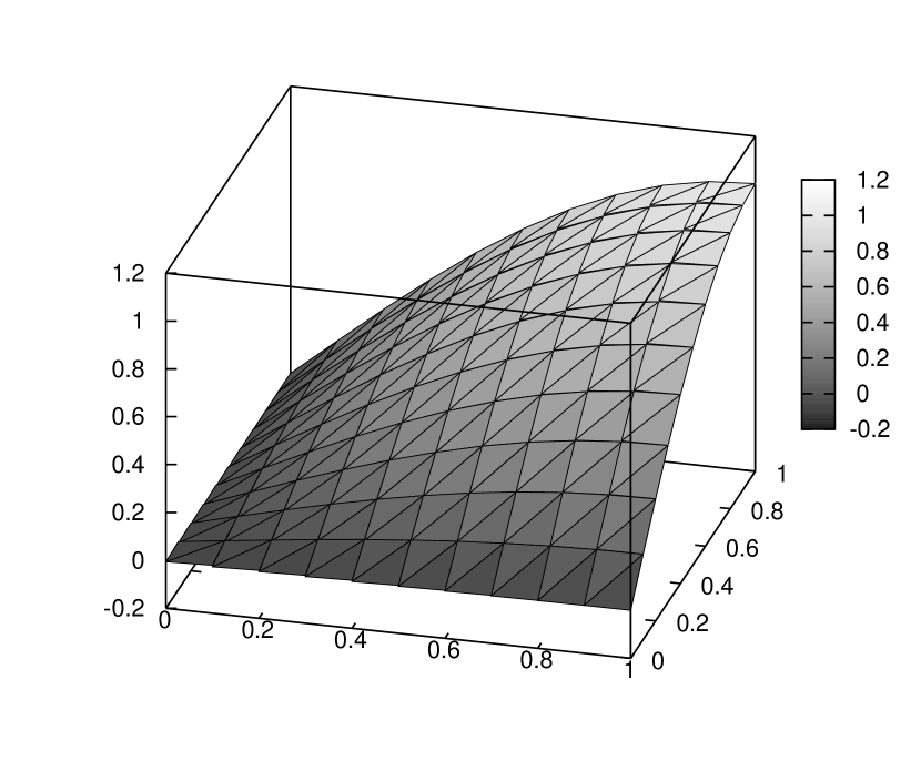
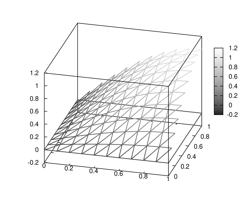
Figure 2: Our HDG solutions $u_{h}$(left) and $\hat{u}_{h}$(right) for $h=1/10$ and $\varepsilon=10^{-6}$.

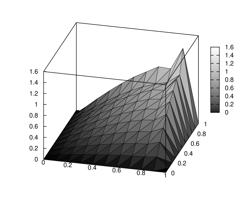
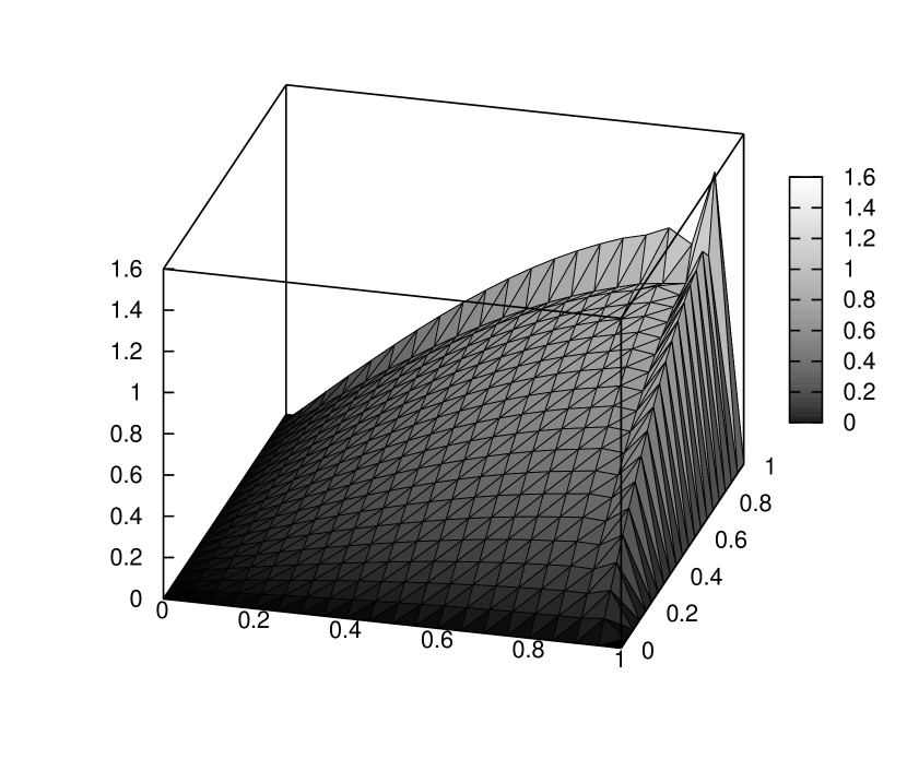
Figure 3: The SUPG solutions for $h=1/10$ (left) and $h=1/20$(right) in the case of $\varepsilon=10^{-6}$.

Figure 4: Convergence diagrams in the boundary layer case. $L^{2}$-errors(top) and $H^{1}(\mathcal{T}_{h})$-errors(bottom) in $\Omega_{0.9}$ for $\varepsilon=10^{-6}$.

6.3 Continuous approximations for $\hat{u}_{h}$

We will present numerical results when continuous funcions are employed for $\hat{u}_{h}$. The same problem in Section 6.2 is considered. Figure 5 displays the graphs of the approximate solutions in the case $\varepsilon=10^{-6}$ and $h=1/10$. It can be seen that overshoots appear near the outflow boundary, which is similar to the result by the SUPG method. This suggests that discontinuous approximations may have better stability properties than continuous ones in the convection-dominated cases.

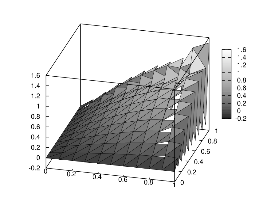
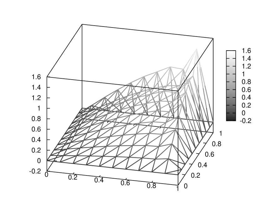
Figure 5: Our HDG solutions in the case that $\hat{u}_{h}$ is continuous: $u_{h}$(left) and $\hat{u}_{h}$(right).

7 Conclusions

We have presented a new derivation of a hybridized scheme for the convection-diffusion problems. In our formulation, an upwinding term is added to satisfy the coercivity of a convective part. As a result, our scheme is stable even when $\varepsilon\downarrow 0$. Indeed, numerical results show that no spurious oscillation appears in our approximate solutions. We have proved the error estimates of optimal order in the HDG norm, and discussed the relation between our approximate solution and an exact one of the reduced problem.

- (1) Adams, R., Fournier, J.: Sobolev Spaces, 2nd edition. Academic Press (2003)
- (2) Arnold, D.N., Brezzi, F., Cockburn, B., Marini, L.D.: Unified analysis of discontinuous Galerkin methods for elliptic problems. SIAM J. Numer. Anal. 39, 1749–1779 (2002)
- (3) Brenner, S.C., Scott, L.R.: The Mathematical Theory of Finite Element Methods, 3rd ed. Springer (2008)
- (4) Brooks, A.N., Hughes, T.J.R.: Streamline upwind/petrov-galerkin formulations for convection dominated flows with particular emphasis on the incompressible navier-stokes equations. Comput. Methods Appl. Mech. Engrn. 32, 199–259 (82)
- (5) Chen, Y., Cockburn, B.: Analysis of variable-degree HDG methods for convection-diffusion equations. part I: General nonconforming meshes. IMA J. Numer. Anal. (To appear.)
- (6) Cockburn, B., Cui, J.: An analysis of HDG methods for the vorticity-velocity-pressure formulation of the Stokes problem in three dimensions. Math. Comp. 81, 1355–1368 (2012)
- (7) Cockburn, B., Cui, J.: Divergence-free HDG methods for the vorticity-velocity formulation of the Stokes problem. J. Sci. Comput. 52, 256–270 (2012)
- (8) Cockburn, B., Dong, B., Guzmán, J.: A superconvergent LDG-hybridizable Galerkin method for second-order elliptic problems. Math. Comp. 77, 1887–1916 (2008)
- (9) Cockburn, B., Dong, B., Guzmán, J., Restelli, M., Sacco, R.: A hybridizable discontinuous Galerkin method for steady-state convection-diffusion-reaction problems. SIAM J. Sci. Comput. 31, 3827–3846 (2009)
- (10) Cockburn, B., Gopalakrishnan, J.: The derivation of hybridizable discontinuous Galerkin methods for Stokes flow. SIAM J. Numer. Anal. 47, 1092–1125 (2009)
- (11) Cockburn, B., Gopalakrishnan, J., Lazarov, R.: Unified hybridization of discontinuous Galerkin, mixed, and continuous Galerkin methods for second order elliptic problems. SIAM J. Numer. Anal. 47, 1319–1365 (2009)
- (12) Cockburn, B., Gopalakrishnan, J., Nguyen, N.C., Peraire, J., Sayas, F.J.: Analysis of HDG methods for Stokes flow. Math. Comp. 80, 723–760 (2011)
- (13) Cockburn, B., Gopalakrishnan, J., Sayas, F.J.: A projection-based error analysis of HDG methods. Math. Comp. 79, 1351–1367 (2010)
- (14) Cockburn, B., Guzmán, J., Soon, S.C., Stolarski, H.K.: An analysis of the embedded discontinuous Galerkin method for second-order elliptic problems. SIAM J. Numer. Anal. 47, 2686–2707 (2009)
- (15) Egger, H., Schöberl, J.: A hybrid mixed discontinuous Galerkin finite element method for convection-diffusion problems. IMA J. Numer. Anal. 30, 1206–1234 (2010)
- (16) John, V., Knobloch, P.: On spurious oscillations at layers diminishing (SOLD) methods for convection–diffusion equations: part I – a review. Comput. Methods Appl. Mech. Engrg. 196, 2197–2215 (2007)
- (17) Kikuchi, F., Ando, Y.: A new variational functional for the finite-element method and its application to plate and shell problems. Nucl. Eng. Des. 21, 95–113 (1972)
- (18) Kikuchi, F., Ando, Y.: Some finite element solutions for plate bending problems by simplified hybrid displacement method. Nucl. Eng. Des. 23, 155–178 (1972)
- (19) Kikuchi, F., Ishii, K., Oikawa, I.: Discontinuous Galerkin FEM of hybrid displacement type – development of polygonal elements. Theo. & Appl. Mech. Japan 57, 395–404 (2009)
- (20) Knabner, P., Angerman, L.: Numerical Methods for Elliptic and Parabolic Partial Differential Equations. Springer New York (2003)
- (21) Knobloch, P.: On the choice of the SUPG parameter at outflow boundary layers. Adv. Comput. Math. 31, 369–389 (2009)
- (22) Labeur, R.J., Wells, G.N.: A Galerkin interface stabilisation method for advection-diffusion and incompressible Navier-Stokes equations. Comput. Methods Appl. Mech. Engrg. 196, 4985–5000 (2007)
- (23) Nguyen, N.C., Peraire, J., Cockburn, B.: An implicit high-order hybridizable discontinuous Galerkin method for linear convection-diffusion equations. J. Comput. Phys. pp. 8841–8855 (2009)
- (24) Nguyen, N.C., Peraire, J., Cockburn, B.: A hybridizable discontinuous Galerkin method for Stokes flow. Comput. Methods Appl. Mech. Engrg. 199, 582–597 (2010)
- (25) Nguyen, N.C., Peraire, J., Cockburn, B.: An implicit high-order hybridizable discontinuous Galerkin method for the incompressible Navier-Stokes equations. J. Comput. Phys. 230, 1147–1170 (2011)
- (26) Oikawa, I.: Discontinuous galerkin fem of hybrid for a convetcion-diffusion problem. Presentation at the Annual Meeting of Japan SIAM Meiji University, Tokyo, Japan (2010)
- (27) Oikawa, I.: Hybridized discontinuous galerkin method for a convection-diffusion problem. Presentation at the Annual Meeting of Japan SIAM Nagoya University, Aichi, Japan (2010)
- (28) Oikawa, I.: Hybridized discontinuous Galerkin method with lifting operator. JSIAM Lett. 2, 99–102 (2010)
- (29) Oikawa, I., Kikuchi, F.: Discontinuous Galerkin FEM of hybrid type. JSIAM Lett 2, 49–52 (2010)
- (30) Pian, T., Wu, C.C.: Hybrid and Incompatible Finite Element Methods. Chapman & Hall (2005)
- (31) Reed, W., Hill, T.: Triangular mesh methods for the neutron transport equation. Tech. rep., Tech. Report LA-UR-73-479 (1973)
- (32) Richter, G.R.: The discontinuous Galerkin method with diffusion. Math. Comp. 58, 631–643 (1992)
- (33) Tong, P.: New displacement hybrid finite element models for solid continua. Int. J. Num. Meth. Eng. 2, 95–113 (1970)
- (34) Wells, G.N.: Analysis of an interface stabilized finite element method: the advection-diffusion-reaction equation. SIAM J. Numer. Anal. 49, 87–109 (2011)