Optimal Checkpointing Period: Time vs. Energy

Abstract

This short paper deals with parallel scientific applications using non-blocking and periodic coordinated checkpointing to enforce resilience. We provide a model and detailed formulas for total execution time and consumed energy. We characterize the optimal period for both objectives, and we assess the range of time/energy trade-offs to be made by instantiating the model with a set of realistic scenarios for Exascale systems. We give a particular emphasis to I/O transfers, because the relative cost of communication is expected to dramatically increase, both in terms of latency and consumed energy, for future Exascale platforms.

1 Introduction

A significant research effort is focusing on the characteristics, features, and challenges of High Performance Computing (HPC) systems capable of reaching the Exaflop performance mark [1, 2]. The portrayed Exascale systems will necessitate billion way parallelism, resulting not only in a massive increase in the number of processing units (cores), but also in terms of computing nodes. Considering the relative slopes describing the evolution of the reliability of individual components on one side, and the evolution of the number of components on the other side, the reliability of the entire platform is expected to decrease, due to probabilistic amplification. Even if each independent component is quite reliable, the Mean Time Between Failures (MTBF) is expected to drop drastically. Executions of large parallel applications on these systems will have to tolerate a higher degree of errors and failures than in current systems. The de-facto general-purpose error recovery technique in high performance computing is checkpoint and rollback recovery. Such protocols employ checkpoints to periodically save the state of a parallel application, so that when an error strikes some process, the application can be restored into one of its former states. The most widely used protocol is coordinated checkpointing, where all processes periodically stop computing and synchronize to write critical application data onto stable storage. Coordinated checkpointing is well understood, at least in its blocking form (when no computing activity takes place during checkpoints), and good approximations of the optimal checkpoint interval exist; they are known as Young’s and Daly’s formula [3, 4].

While reliability is a major concern for Exascale, another key challenge is to minimize energy consumption, both for economic and environmental reasons. One of the most power-consuming components of today’s systems is the processor: even when idle, it dissipates a significant fraction of the total power. However, for future Exascale systems, the power dissipated to execute I/O transfers is likely to play an even more important role, because the relative cost of communication is expected to dramatically increase, both in terms of latency and consumed energy [5].

In this short paper, we investigate trade-offs between execution time and energy consumption for the execution of parallel applications on future Exascale systems. The optimal period $\mathcal{T}_{\text{Time}}^{\text{opt}}$ given by Young’s and Daly’s formula [3, 4] will minimize (expected) execution time. But will it minimize energy consumption? The answer is negative, mainly because the fraction of power $\mathcal{P}_{\text{Cal}}$ spent when computing (by the CPUs) is not the same as the fraction of power $\mathcal{P}_{\text{I/O}}$ spent when checkpointing. In particular, we revisit the work of Meneses, Sarood and Kalé [6] for checkpoint/restart, where formulas are given to compute the time-optimum and energy-optimum periods. However, our model is more precise: (i) we carefully assess the impact of the power consumption required for I/O activity, which is likely to play a key role at the Exascale; (ii) we consider non-blocking checkpointing that can be partially overlapped with computations; (iii) we give a more accurate analysis of the consumed energy.

Altogether, this short paper provides the following main contributions:

• We provide a refined analytical model to compute both the execution time and the consumed energy with a given checkpoint period. The model handles the case where checkpointing activity can be non-blocking, i.e., partially overlapped with computations.

• We provide analytical formulas to approximate the optimal period for time $\mathcal{T}_{\text{Time}}^{\text{opt}}$ as well as the optimal period for energy $\mathcal{T}_{\text{Energy}}^{\text{opt}}$, thereby refining and extending Daly [4] and Meneses, Sarood and Kalé [6] results to non-blocking checkpoints.

• We assess the range of time/energy trade-offs to be made by instantiating the model with a set of realistic scenarios for Exascale systems.

2 Model

In this section, we introduce all the model parameters. We start with parameters related to resilience (checkpointing) before moving to parameters related to energy consumption.

2.1 Checkpointing

We model coordinated checkpointing [7] where checkpoints are taken at regular intervals, after some fixed amount of work units have been performed. This corresponds to an execution partitioned into periods of duration $T$. Every period, a checkpoint of length $C$ is taken.

An important question is whether checkpoints are blocking or not. On some architectures, we may have to stop executing the application before writing to the stable storage where the checkpoint data is saved; in that case checkpoint is fully blocking. On other architectures, checkpoint data can be saved on the fly into a local memory before the checkpoint is sent to the stable storage, while computation can resume progress; in that case, checkpoints can be fully overlapped with computations. To deal with all situations, we introduce a slow-down factor $\omega$: during a checkpoint of duration $C$, the work that is performed is $\omega C$ work units. In other words, $(1-\omega)C$ work units are wasted due to checkpoint jitter disrupting the progress of computation. Here, $0\leq\omega\leq 1$ is an arbitrary parameter. The case $\omega=0$ corresponds to a fully blocking checkpoint, while $\omega=1$ corresponds to a checkpoint totally overlapped with computations. All intermediate situations can be represented.

Next we have to account for failures. During $t$ time units of execution, the expectation of the number of failures is $\frac{t}{\mu}$, where $\mu$ is the MTBF (Mean Time Between Failures) of the platform. Note that if the platform if made of $N$ identical resources whose individual mean time between failures is $\mu_{\text{ind}}$, then $\mu=\frac{\mu_{\text{ind}}}{N}$. This relation is agnostic of the granularity of the resources, which can be anything from a single CPU to a complex multi-core socket. When a failure strikes, there is a downtime of length $D$ (time to reboot the resource or set up a spare), and then a recovery of length $R$ (time to read the last stored checkpoint). The work executed by the application since the last checkpoint and before the failure needs to be re-executed. Clearly, the shorter the period $T$, the less work to re-execute, but also the more overhead due to frequent checkpoints in a failure-free execution. The best trade-off when $\omega=0$ (blocking checkpoint) is achieved for $T=\sqrt{2C\mu}+C$ (Young’s formula  [3]) or $T=\sqrt{2C(\mu+D+R)}+C$ (Daly’s formula [4]). Both formulas are first-order approximations and valid only if all checkpoint parameters $C$, $D$ and $R$ are small in front of $\mu$ (and these formulas collapse if they become negligible). In Section 3, we show how to extend these formulas to the case of non-blocking checkpoints (see also [8] for more details).

2.2 Energy

To compute the energy consumption of the application, we need to consider the energy consumption of the different phases, and hence the power consumption at each time-step. To this purpose, we define:

• $\mathcal{P}_{\text{Static}}$ : this is the base power consumed when the platform is switched on.

• $\mathcal{P}_{\text{Cal}}$ : when the platform is active, we have to consider the CPU overhead in addition to the static power $\mathcal{P}_{\text{Static}}$.

• $\mathcal{P}_{\text{I/O}}$ : similarly, this is the power overhead due to file I/O. This supplementary power consumption is induced by checkpointing, or when recovering from a failure.

• $\mathcal{P}_{\text{Down}}$ : for coordinated checkpointing, when one processor fails, the rest of the machine stays idle. $\mathcal{P}_{\text{Down}}$ is the power consumption overhead when one machine is down, that may be incurred for instance by rebooting the machine. In general, we let $\mathcal{P}_{\text{Down}}=0$.

Meneses, Sarood and Kalé [6] have a simpler model with two parameters, namely $L$, the base power (corresponding to $\mathcal{P}_{\text{Static}}$ with our notations), and $H$, the maximum power (corresponding to $\mathcal{P}_{\text{Static}}+\mathcal{P}_{\text{Cal}}$ with our notations). They use $\mathcal{P}_{\text{I/O}}=\mathcal{P}_{\text{Down}}=0$.

In Section 3, we show how to compute the optimal period that minimizes the energy consumption. In Section 4, we instantiate the model with expected values for power consumption of Exascale platforms.

3 Optimal checkpointing period

We consider a parallel application whose execution time is $\mathcal{T}_{\text{base}}$ without any overhead due to the resilience method or the occurrence of failures. We compute the expectation $\mathcal{T}_{\text{final}}$ of the total execution time (accounting both for checkpointing and for failures) in Section 3.1, and the expectation $\mathcal{E}_{\text{final}}$ of the total energy consumed during this execution of length $\mathcal{T}_{\text{final}}$ in Section 3.2. We will compute the optimal period $T$ that minimizes the objective, either $\mathcal{T}_{\text{final}}$ or $\mathcal{E}_{\text{final}}$.

3.1 Execution time

The total execution time $\mathcal{T}_{\text{final}}$ of the application depends on two sources of overhead. We first compute $\mathcal{T}_{\text{ff}}$, the time taken by a fault-free execution, thereby accounting only for the overhead due to periodic checkpointing. Then we compute $\mathcal{T}_{\text{fails}}$, the time lost due to failures. Finally, $\mathcal{T}_{\text{final}}=\mathcal{T}_{\text{ff}}+\mathcal{T}_{\text{fails}}$. We detail here both computations:

• The reasoning to derive $\mathcal{T}_{\text{ff}}$ is simple. We need to execute a total amount of work equal to $\mathcal{T}_{\text{base}}$. During each period of length $T$, there is an amount of time $T-C$ where only computations take place, and an amount of time $C$ of checkpointing, where only a work $\omega C$ is done. Therefore, the total number of work units executed during a period of length $T$ is $T-C+\omega C=T-(1-\omega)C$, and
  

  $$\mathcal{T}_{\text{ff}}=\mathcal{T}_{\text{base}}\frac{T}{T-(1-\omega)C}.$$

• The reasoning to compute $\mathcal{T}_{\text{fails}}$ is the following. Since the mean time between two failures is $\mu$, the average number of failures during execution is $\frac{\mathcal{T}_{\text{final}}}{\mu}$. For each failure, the time lost is expressed as:

  • $D+R$ for downtime and recovery;

  • a time $\omega C$ for the work that was done during the previous checkpoint and that has to be redone because it was not checkpointed (because of the failure);

  • with probability $\frac{T-C}{T}$, the failure happens while we are not checkpointing, and the time lost is on average $A=\frac{T-C}{2}$;

  • otherwise, with probability $\frac{C}{T}$, the failure happens while we are checkpointing, and the time lost is on average $B=T-C+\frac{C}{2}=T-\frac{C}{2}$.

  The time lost for each failure is

  $$D+R+\omega C+\frac{T-C}{T}A+\frac{C}{T}B=D+R+\omega C+\frac{T}{2}.$$

  Finally,
  

  $$\mathcal{T}_{\text{fails}} =\frac{\mathcal{T}_{\text{final}}}{\mu}\left(D+R+\omega C+\frac{T}{2}\right).$$

We are now ready to express the total execution time:

$$\mathcal{T}_{\text{final}} =\mathcal{T}_{\text{ff}}+\mathcal{T}_{\text{fails}}$$

$$=\mathcal{T}_{\text{base}}\frac{T}{T-(1-\omega)C}+\frac{\mathcal{T}_{\text{final}}}{\mu}\left(D+R+\omega C+\frac{T}{2}\right)$$

$$=\frac{T}{\left(T-(1-\omega)C\right)\left(1-\frac{D+R+\omega C+T/2}{\mu}\right)}\mathcal{T}_{\text{base}}$$

$$=\frac{T}{\left(T-a\right)\left(b-\frac{T}{2\mu}\right)}\mathcal{T}_{\text{base}},$$

where $a=(1-\omega)C$ and $b=1-\frac{D+R+\omega C}{\mu}$.

This equation is minimized for

$$\mathcal{T}_{\text{Time}}^{\text{opt}}=\sqrt{2(1-\omega)C(\mu-(D+R+\omega C))}.$$ (1)

When $\omega=0$, we obtain an expression close to that of Young and Daly, but slightly different because they have less accurately approximated the total execution time. In the following, we let AlgoT be the checkpointing strategy that checkpoints with period $\mathcal{T}_{\text{Time}}^{\text{opt}}$.

3.2 Energy consumption

In order to compute the total energy consumption of the execution, we consider the different phases during which the different powers introduced in Section 2.2 are used:

• First, we consume $\mathcal{P}_{\text{Static}}$ during each time-step of the execution. Indeed, even when a node fails and is shutdown, we still pay for the power of all the other nodes, for the cooling system, etc. The corresponding energy cost is $\mathcal{T}_{\text{final}}\mathcal{P}_{\text{Static}}$.

• Next, let $\mathcal{T}_{\text{Cal}}$ be the time during which the CPU is used, inducing a power overhead $\mathcal{P}_{\text{Cal}}$. $\mathcal{T}_{\text{Cal}}$ includes the base work $\mathcal{T}_{\text{base}}$, and $\mathcal{T}_{\text{re-exec}}$, the work that must be re-executed after each failure (which we multiply by the number of failures $\mathcal{T}_{\text{final}}/\mu$):

  • with probability $\frac{T-C}{T}$, the failure does not happen during a checkpoint, and the work to re-execute is $A=\omega C+\frac{T-C}{2}$;

  • with probability $\frac{C}{T}$, the failure happens during the execution of a checkpoint, and the work to re-execute is $B=\omega C+T-C+\frac{\omega C}{2}$.

  We derive $\mathcal{T}_{\text{re-exec}}=\frac{T-C}{T}A+\frac{C}{T}B$, hence
  

  $$\mathcal{T}_{\text{re-exec}}=\omega C+\frac{T^{2}-C^{2}}{2T}+\frac{\omega C^{2}}{2T}.$$

  Finally, we have:

  $$\mathcal{T}_{\text{Cal}}=\mathcal{T}_{\text{base}}+\frac{\mathcal{T}_{\text{final}}}{\mu}\left(\omega C+\frac{T^{2}-C^{2}}{2T}+\frac{\omega C^{2}}{2T}\right).$$

  The corresponding energy consumption is $\mathcal{T}_{\text{Cal}}\mathcal{P}_{\text{Cal}}$.

• Let $\mathcal{T}_{\text{I/O}}$ be the time during which the I/O system is used, inducing a power overhead $\mathcal{P}_{\text{I/O}}$. This time corresponds to checkpointing and recovery from failures.

  • The total number of checkpoints that are taken in a fault-free execution is equal to the number of periods, $\frac{\mathcal{T}_{\text{base}}}{T-(1-\omega)C}$, and the time taken by checkpoints is therefore $\frac{\mathcal{T}_{\text{base}}C}{T-(1-\omega)C}$.

  • For each failure, there is an additional overhead:

    1. the system needs to recover, which lasts $R$ time-steps;

    2. with probability $\frac{T-C}{T}$, the failure does not happen during a checkpoint, and there is no additional I/O overhead;

    3. however, with probability $\frac{C}{T}$, the failure happens during a checkpoint, and the I/O time wasted is (in average) $\frac{C}{2}$.

  Altogether, we obtain

  $$\mathcal{T}_{\text{I/O}}=\frac{\mathcal{T}_{\text{base}}C}{T-(1-\omega)C}+\frac{\mathcal{T}_{\text{final}}}{\mu}\left(R+\frac{C^{2}}{2T}\right).$$

  The corresponding energy consumption is $\mathcal{T}_{\text{I/O}}\mathcal{P}_{\text{I/O}}$.

• Finally, let $\mathcal{T}_{\text{Down}}$ be the total down time, incurring a power overhead $\mathcal{P}_{\text{Down}}$. We have

  $$\mathcal{T}_{\text{Down}}=\frac{\mathcal{T}_{\text{final}}}{\mu}D,$$

  and the corresponding energy cost is $\mathcal{T}_{\text{Down}}\mathcal{P}_{\text{Down}}$. This term is only included for full generality, as we expect to have $\mathcal{P}_{\text{Down}}=0$ in most scenarios.

The final expression for the total energy consumed is

$$\mathcal{E}_{\text{final}} =\mathcal{T}_{\text{Cal}}\mathcal{P}_{\text{Cal}}+\mathcal{T}_{\text{I/O}}\mathcal{P}_{\text{I/O}}+\mathcal{T}_{\text{Down}}\mathcal{P}_{\text{Down}}+\mathcal{T}_{\text{final}}\mathcal{P}_{\text{Static}}$$

$$=\left(\mathcal{T}_{\text{base}}+\frac{\mathcal{T}_{\text{final}}}{\mu}\left(\omega C+\frac{T^{2}-C^{2}}{2T}+\frac{\omega C^{2}}{2T}\right)\right)\mathcal{P}_{\text{Cal}}$$

$$\quad+\left(\frac{\mathcal{T}_{\text{final}}}{\mu}\left(R+\frac{C^{2}}{2T}\right)+C\frac{\mathcal{T}_{\text{base}}}{T-(1-\omega)C}\right)\mathcal{P}_{\text{I/O}}$$

$$\quad+\frac{\mathcal{T}_{\text{final}}}{\mu}D\mathcal{P}_{\text{Down}}+\mathcal{T}_{\text{final}}\mathcal{P}_{\text{Static}}.$$

It is important to understand that $\mathcal{T}_{\text{final}}\neq\mathcal{T}_{\text{Cal}}+\mathcal{T}_{\text{I/O}}+\mathcal{T}_{\text{Down}}$, unless $\omega=0$. Indeed, CPU and I/O activities are overlapped (and both consumed) when checkpointing. To ease the derivation of the optimal period that minimizes $\mathcal{E}_{\text{final}}$, we introduce some notations and let $\mathcal{P}_{\text{Cal}}=\alpha\mathcal{P}_{\text{Static}}$, $\mathcal{P}_{\text{I/O}}=\beta\mathcal{P}_{\text{Static}}$, and $\mathcal{P}_{\text{Down}}=\gamma\mathcal{P}_{\text{Static}}$. Re-using parameters $a=(1-\omega)C$ and $b=1-\frac{D+R+\omega C}{\mu}$ from Section 3.1, we obtain:

$$\frac{\mathcal{T}_{\text{final}}^{\prime}}{\mathcal{T}_{\text{base}}}=\frac{-ab+\frac{T^{2}}{2\mu}}{\left(T-a\right)^{2}\left(b-\frac{T}{2\mu}\right)^{2}},\text{\leavevmode\nobreak\ \leavevmode\nobreak\ \leavevmode\nobreak\ \leavevmode\nobreak\ \leavevmode\nobreak\ and}$$

$$\frac{\mathcal{E}_{\text{final}}^{\prime}}{\mathcal{P}_{\text{Static}}} \!\!\!=\!\frac{\mathcal{T}_{\text{final}}^{\prime}}{\mu}\!\left(\alpha\omega C\!+\!\beta R\!+\!\gamma D\!+\!\frac{\alpha T}{2}\!-\!\frac{\alpha(1-\omega)C^{2}}{2T}\!+\!\frac{\beta C^{2}}{2T}\!+\!\mu\right)$$

$$+\frac{\mathcal{T}_{\text{final}}}{2\mu}\left(\alpha\!+\!\frac{\alpha(1-\omega)C^{2}}{T^{2}}\!-\!\frac{\beta C^{2}}{T^{2}}\right)\!-\!\frac{\beta C\mathcal{T}_{\text{base}}}{\left(T\!-\!(1\!-\!\omega)C\right)^{2}}.$$

Then, letting $K=\frac{\left(T-a\right)^{2}\left(b-\frac{T}{2\mu}\right)^{2}}{\mathcal{P}_{\text{Static}}\mathcal{T}_{\text{base}}}$, we have:

$$K\mathcal{E}_{\text{final}}^{\prime} =\frac{-ab\!+\!\frac{T^{2}}{2\mu}}{\mu}\!\!\left(\!\left(\alpha\omega C\!+\!\beta R\!+\!\gamma D\!+\!\mu\right)\!+\!\frac{\alpha T}{2}\!+\!\frac{\alpha(1-\omega)C^{2}}{2T}\!+\!\frac{\beta C^{2}}{2T}\!\right)$$

$$\quad+\frac{\left(T\!-\!a\right)\!(b\!-\!\frac{T}{2\mu})}{2\mu}\!\!\left(\alpha\!+\!\frac{\alpha(1-\omega)C^{2}\!-\!\beta C^{2}}{T}\right)\!-\!\beta C\left(b\!-\!\frac{T}{2\mu}\right)^{2}$$

$$=T^{3}\!\!\left(\!\frac{1}{4\mu}\!-\!\frac{1}{4\mu}\!\right)\!+\!T^{2}\!\!\left(\frac{\alpha\omega C\!+\!\beta R\!+\!\gamma D}{2\mu^{2}}\!+\!\frac{b\!+\!\frac{a}{2\mu}}{2\mu}\!-\!\frac{\beta C}{4\mu^{2}}\!+\!\frac{1}{2\mu}\right)$$

$$\quad+T\left(\!-\!\frac{ab}{2\mu}\!-\!\frac{ab}{2\mu}\!+\!\frac{\beta Cb}{\mu}\!-\!2\frac{(\alpha(1-\omega)\!-\!\beta)C^{2}}{4\mu^{2}}\right)\!-\!\beta Cb^{2}$$

$$\quad-\frac{ab\left(\alpha\omega C\!+\!\beta R\!+\!\gamma D\!+\!\mu\right)}{\mu}\!-\!\left(\frac{b}{2\mu}\!-\!\frac{a}{4\mu^{2}}\right)\!(\alpha(1-\omega)\!-\!\beta)C^{2}$$

$$\quad+\frac{1}{T}\!\!\left(\left(\alpha(1-\omega)\!-\!\beta\right)\frac{C}{2\mu}\!-\!\left(\alpha(1-\omega)\!-\!\beta\right)\frac{C}{2\mu}\right)$$

$$=T^{2}\left(\frac{\alpha\omega C\!+\!\beta R\!+\!\gamma D}{2\mu^{2}}\!+\!\frac{b}{2\mu}\!+\!\frac{a\!-\!\beta C}{4\mu^{2}}\!+\!\frac{1}{2\mu}\right)$$

$$\quad+T\left(\frac{(\beta C\!-\!a)b}{\mu}\!-\!2\frac{(\alpha(1-\omega)\!-\!\beta)C^{2}}{4\mu^{2}}\right)$$

$$\quad-\frac{ab\left(\alpha\omega C\!+\!\beta R\!+\!\gamma D\!+\!\mu\right)}{\mu}\!-\!\beta Cb^{2}$$

$$\quad+\left(\frac{b}{2\mu}\!+\!\frac{a}{4\mu^{2}}\right)\!(\alpha(1-\omega)\!-\!\beta)C^{2}\;.$$

Let $\mathcal{T}_{\text{Energy}}^{\text{opt}}$ be the only positive root of this quadratic polynomial in $T$: $\mathcal{T}_{\text{Energy}}^{\text{opt}}$ is the value that minimizes $\mathcal{E}_{\text{final}}$. In the following, we let AlgoE be the checkpointing strategy that checkpoints with period $\mathcal{T}_{\text{Energy}}^{\text{opt}}$.

As a side note, let us emphasize the differences with the approach of Meneses, Sarood and Kalé [6] when restricting to the case $\omega=0$ (because they only consider the blocking variant). For each failure, they consider that:

• energy lost due to re-execution is $\frac{T-2C}{2}\mathcal{P}_{\text{Cal}}$, while we have

  $$\left(\frac{T-C}{T}\left(\frac{T-C}{2}\right)+\frac{C}{T}\left(T-C\right)\right)\mathcal{P}_{\text{Cal}}=\frac{T^{2}-C^{2}}{2T}\mathcal{P}_{\text{Cal}}$$

• energy lost due to I/O is $C\mathcal{P}_{\text{I/O}}$, while we have $\frac{C^{2}}{2T}\mathcal{P}_{\text{I/O}}$.

Theses differences come from our more detailed analysis of the impact of the failure location, which can strike either during the computation phase, or during the checkpointing phase, of the whole period.

4 Experiments

In this section, we instantiate the previous model with scenarios taken from current projections for Exascale platforms [1, 2, 5, 9]. We choose realistic values for all model parameters: this includes all types of power consumption ($\mathcal{P}_{\text{Static}}$, $\mathcal{P}_{\text{Cal}}$, $\mathcal{P}_{\text{I/O}}$ and $\mathcal{P}_{\text{Down}}$), all checkpoint parameters ($C$, $R$, $D$ and $\omega$), and the platform MTBF $\mu$. We start with a word of caution: our choices for these parameters may be somewhat arbitrary, and do not cover the whole range of scenarios that can be investigated. However, a key feature of our model is its robustness: as long as $\mu$ is reasonably large in front of checkpoint times, the model is able to accurately predict the best period for execution time and for energy consumption.

The power consumption of an Exascale machine is capped to $20$ Mega-watts. With $10^{6}$ nodes, this represents a nominal power of $20$ milli-watts per node. Let us express all power values in milli-watts. A reasonable scenario is to assume that half this power is used for operating the platform, hence to let $\mathcal{P}_{\text{Static}}=10$. The overhead due to computing would represent the other half, hence $\mathcal{P}_{\text{Cal}}=10$. As for communications and I/Os, which are expected to cost an order of magnitude more than computing [5], we take an overhead of $100$, hence $\mathcal{P}_{\text{I/O}}=100$. A key parameter for the experimental study is the ratio

$$\ratio=\frac{\mathcal{P}_{\text{Static}}+\mathcal{P}_{\text{I/O}}}{\mathcal{P}_{\text{Static}}+\mathcal{P}_{\text{Cal}}}=\frac{1+\beta}{1+\alpha}.$$ (2)

With our values, we get $\ratio=5.5$. Note that if we used $\mathcal{P}_{\text{Static}}=5$ and kept the same overheads $10$ and $100$ for computing and I/O respectively, we would get $\mathcal{P}_{\text{Cal}}=10$, $\mathcal{P}_{\text{I/O}}=100$, and $\ratio=7$. These two representative values of  ($\ratio=5.5$ and $\ratio=7$) are emphasized by vertical arrows in the plots below on Figure 1. As for $\mathcal{P}_{\text{Down}}$, the power during downtime, we use $\mathcal{P}_{\text{Down}}=0$, meaning that during downtime we only account for the static power $\mathcal{P}_{\text{Static}}$ of the processors that are idle.

The Jaguar platform, with $N=45,208$ processors, is reported to have experienced about one fault per day [10], which leads to an individual (processor) MTBF $\mu_{\text{ind}}$ equal to $\frac{45,208}{365}\approx 125$ years. Therefore, we set the individual (processor) MTBF to $\mu_{\text{ind}}=125$ years. Letting the total number of processors $N$ vary from $N=219,150$ to $N=2,191,500$ (future exascale platforms), the platform MTBF $\mu$ varies from $\mu=300$ min ($5$ hours) down to $\mu=30$ min. The experiments use resilience parameters that are representative of current and forthcoming large-scale platforms [9, 11]. We take $C=R=10$ min, $D=1$ min, and $\omega=1/2$.

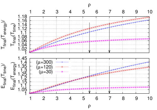
Figure 1: Time and energy ratios as a function of , with $C=R=10$ min, $D=1$ min, $\gamma=0$, $\omega=1/2$, and various values for $\mu$.

On Figures 1 and 2, we evaluate the impact of the ratio  (see Equation (2)) on the gain in energy and loss in time of AlgoE with respect to AlgoT. The general trend is that using AlgoE can lead to significant gains in energy at the price of a small increase in execution time.

We then study in Figure 3 the scalability of the approach on forthcoming platforms. We set the duration of the complete checkpoint and rollback ($C$ and $R$, respectively) to $1$ minute, independently of the number of processors, and we let the downtime $D$ equal to $0.1$ minutes. It is reasonable to consider that checkpoint storage time will not increase with the number of nodes in the future, but on the contrary will remain constant. Indeed, system designers are studying a couple of alternative approaches. One consists in featuring each computing node with local storage capability, ensuring through the hardware that this storage will remain available during a failure of the node. Another approach consists in using the memory of the other processors to store the checkpoint, pairing nodes as “buddies”, thus allowing to take advantage of the high bandwidth capability of the high speed network to design a scalable checkpoint storage mechanism [12, 13, 14, 15].

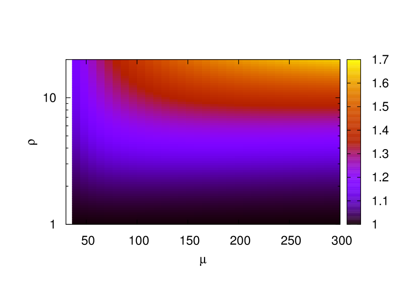
(a) Energy ratio of AlgoT over AlgoE

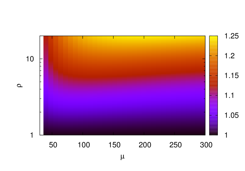
(b) Execution time ratio of AlgoE over AlgoT

Figure 2: Ratios of the different strategies with $C=R=10$ min, $D=1$ min, $\gamma=0$, $\omega=1/2$ as a function of $\mu$ and .

The MTBF for $10^{6}$ nodes is set to $2$ hours, and this value scales linearly with the number of components. Given these parameters, Figures 3(a) and 3(b) shows (i) the execution time ratio of AlgoE over AlgoT, and (ii) the energy consumption ratio of AlgoT over AlgoE, both as a function of the number of nodes. Figures 3(a) and 3(b) confirm the important gain in energy that can be achieved, namely up to $30\%$ for a time overhead of only $12\%$. When the number of nodes gets very high (up to $10^{8}$), then we observe that both energy and time ratios converge to $1$. Indeed, when $C$ becomes of the order of magnitude of the MTBF, then both periods $\mathcal{T}_{\text{Time}}^{\text{opt}}$ and $\mathcal{T}_{\text{Energy}}^{\text{opt}}$ become close to $C$ to account for the higher failure rate.

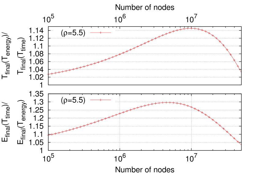
(a) Time and energy ratios, as a function of the number of nodes, when $\ratio=5.5$

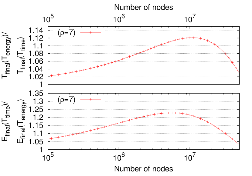
(b) Time and energy ratios, as a function of the number of nodes, when $\ratio=7$

Figure 3: Ratios of total energy and time for the two period strategies, as a function of the number of nodes, with $\mu=120$ min for $10^{6}$ nodes, $C=R=1$ min, $D=0.1$ min, $\gamma=0$, $\omega=1/2$.

5 Conclusion

In this short paper, we have provided a detailed analysis to compute the optimal checkpointing period, when the checkpointing activity can be partially overlapped with computations. We have considered two distinct objectives: either the goal is to minimize the total execution time, or it is to minimize the total energy consumption. Because of the different power consumption overheads due to computations and I/Os, we obtain different optimal periods.

We have instantiated the formulas with values derived from current and future Exascale platforms, and we have studied the impact of the power overhead due to I/O activity on the gains in time and energy. With current values, we can save more than $20\%$ of energy with an MTBF of 300 min, at the price of an increase of $10\%$ in the execution time. The maximum gains are expected for a platform with between $10^{6}$ and $10^{7}$ processors (up to $30\%$ energy savings).

Our analytical model is quite flexible and can easily be instantiated to investigate scenarios that involve a variety of resilience and power consumption parameters.

References

- [1] J. Dongarra, P. Beckman, P. Aerts, F. Cappello, T. Lippert, S. Matsuoka, P. Messina, T. Moore, R. Stevens, A. Trefethen, and M. Valero, “The international exascale software project: a call to cooperative action by the global high-performance community,” Int. Journal of High Performance Computing Applications, vol. 23, no. 4, pp. 309–322, 2009.
- [2] V. Sarkar et al., “Exascale software study: Software challenges in extreme scale systems,” 2009, white paper available at: http://users.ece.gatech.edu/mrichard/ExascaleComputingStudyReports/ECSS%20report%20101909.pdf.
- [3] J. W. Young, “A first order approximation to the optimum checkpoint interval,” Comm. of the ACM, vol. 17, no. 9, pp. 530–531, 1974.
- [4] J. T. Daly, “A higher order estimate of the optimum checkpoint interval for restart dumps,” FGCS, vol. 22, no. 3, pp. 303–312, 2004.
- [5] J. Shalf, S. Dosanjh, and J. Morrison, “Exascale computing technology challenges,” in VECPAR’10, the 9th Int. Conf. High Performance Computing for Computational Science, ser. LNCS 6449. Springer-Verlag, 2011, pp. 1–25.
- [6] E. Meneses, O. Sarood, and L. V. Kalé, “Assessing Energy Efficiency of Fault Tolerance Protocols for HPC Systems,” in Proceedings of the 2012 IEEE 24th International Symposium on Computer Architecture and High Performance Computing (SBAC-PAD 2012), New York, USA, October 2012.
- [7] K. M. Chandy and L. Lamport, “Distributed snapshots: Determining global states of distributed systems,” in Transactions on Computer Systems, vol. 3(1). ACM, February 1985, pp. 63–75.
- [8] G. Bosilca, A. Bouteiller, E. Brunet, F. Cappello, J. Dongarra, A. Guermouche, T. Hérault, Y. Robert, F. Vivien, and D. Zaidouni, “Unified model for assessing checkpointing protocols at extreme-scale,” Concurrency and Computation: Practice and Experience, October 2013, to be published. Also available as INRIA research report 7950 at graal.ens-lyon.fr/~yrobert.
- [9] K. Ferreira, J. Stearley, J. H. I. Laros, R. Oldfield, K. Pedretti, R. Brightwell, R. Riesen, P. G. Bridges, and D. Arnold, “Evaluating the Viability of Process Replication Reliability for Exascale Systems,” in Proc. of the ACM/IEEE SC Conf., 2011.
- [10] G. Zheng, X. Ni, and L. V. Kalé, “A scalable double in-memory checkpoint and restart scheme towards exascale,” in Dependable Systems and Networks Workshops (DSN-W), 2012.
- [11] F. Cappello, H. Casanova, and Y. Robert, “Preventive migration vs. preventive checkpointing for extreme scale supercomputers,” Parallel Processing Letters, vol. 21, no. 2, pp. 111–132, 2011.
- [12] G. Zheng, L. Shi, and L. V. Kalé, “FTC-Charm++: an in-memory checkpoint-based fault tolerant runtime for Charm++ and MPI,” in Proc. 2004 IEEE Int. Conf. Cluster Computing. IEEE Computer Society, 2004.
- [13] X. Ni, E. Meneses, and L. V. Kalé, “Hiding checkpoint overhead in HPC applications with a semi-blocking algorithm,” in Proc. 2012 IEEE Int. Conf. Cluster Computing. IEEE Computer Society, 2012.
- [14] J. Dongarra, T. Hérault, and Y. Robert, “Revisiting the double checkpointing algorithm,” in 15th Workshop on Advances in Parallel and Distributed Computational Models APDCM 2013. IEEE Computer Society Press, 2013.
- [15] R. Rajachandrasekar, A. Moody, K. Mohror, and D. K. D. Panda, “A 1 PB/s file system to checkpoint three million MPI tasks,” in Proceedings of the 22nd international symposium on High-performance parallel and distributed computing, ser. HPDC ’13. New York, NY, USA: ACM, 2013, pp. 143–154.