UWThPh-2013-28

Approximating chiral SU(3) amplitudes

G. Ecker¹, P. Masjuan² and H. Neufeld¹

¹⁾ University of Vienna, Faculty of Physics, Boltzmanngasse 5, A-1090 Wien, Austria

²⁾ Institut für Kernphysik, Johannes Gutenberg-Universität, D-55099 Mainz, Germany

We construct large-$N_{c}$ motivated approximate chiral $SU(3)$ amplitudes of next-to-next-to-leading order. The amplitudes are independent of the renormalization scale. Fitting lattice data with those amplitudes allows for the extraction of chiral coupling constants with the correct scale dependence. The differences between approximate and full amplitudes are required to be at most of the order of N³LO contributions numerically. Applying the approximate expressions to recent lattice data for meson decay constants, we determine several chiral couplings with good precision. In particular, we obtain a value for $F_{0}$, the meson decay constant in the chiral $SU(3)$ limit, that is more precise than all presently available determinations.

1 Introduction

Hadronic processes at low energies cannot be treated with perturbative QCD. The main protagonists in this field, lattice QCD and chiral perturbation theory (CHPT), have mutually benefited from a cooperation started several years ago. The emphasis of this cooperation has shifted in recent years. Although extrapolation to the physical quark (and hadron) masses and finite-volume corrections, both accessible in CHPT, are still useful for lattice simulations, improved computing facilities and lattice algorithms allow for simulations with ever smaller quark masses and larger volumes. On the other hand, the input of lattice QCD for CHPT has become more important over the years to determine the coupling constants of chiral Lagrangians, the so-called low-energy constants (LECs). This input is especially welcome for LECs modulating quark mass terms: unlike in phenomenological analyses, quark (and hadron) masses can be tuned on the lattice.

While this program has been very successful for chiral $SU(2)$, the situation is less satisfactory for $SU(3)$ [1]. In the latter case, the natural expansion parameter (in the meson sector) is $M_{K}^{2}/16\pi^{2}F_{\pi}^{2}\simeq 0.2$. To match the precision that lattice studies can attain nowadays, it is therefore mandatory to include NNLO contributions in CHPT. Although NNLO amplitudes are available for most quantities of interest for lattice simulations [2], there has been a certain reluctance in the lattice community to make full use of those amplitudes for two reasons mainly: for chiral $SU(3)$, NNLO amplitudes are usually quite involved and they are mostly available in numerical form only.

In this paper, we resume our proposal [3] for large-$N_{c}$ motivated approximations of NNLO amplitudes that contain one-loop functions only. Besides recapitulating the main features of those analytic approximations, the following issues will be discussed.

• We set up numerical criteria for the amplitudes to qualify as acceptable approximations. Those criteria can be checked by comparing with available numerical results making use of the full NNLO amplitudes for some given sets of meson masses.

• The proposed approximation includes all terms leading and next-to-leading order in large $N_{c}$. In addition, it contains all chiral logs, independently of the large-$N_{c}$ counting. In order to meet the numerical criteria just mentioned, it may sometimes be useful to go beyond the strict large-$N_{c}$ counting by including also products of one-loop functions occurring in two-loop diagrams.

• In addition to the ratio $F_{K}/F_{\pi}$ of meson decay constants investigated in Ref. [3], here we also study the pion decay constant $F_{\pi}$ itself. By confronting our approximation with lattice data, we demonstrate the possibilities to extract information on both NLO and NNLO LECs. While the NNLO LECs have the expected large uncertainties, the NLO LECs can be determined quite well. Our numerical fits of lattice data are not intended to compete with actual lattice results for obvious reasons. Instead, we hope to encourage lattice groups to use NNLO amplitudes that are much simpler than the full amplitudes and yet offer considerably more insight than, e.g., polynomial fits. These amplitudes can also be considered as relatively simple tools to study convergence issues of chiral $SU(3)$ with lattice data.

In Sec. 2 we review the structure and the salient features of the approximate form of NNLO amplitudes for chiral $SU(3)$ proposed in Ref. [3]. In addition to setting up a criterion for deciding whether the approximation is acceptable for a given observable, we also suggest a possible modification of the original version. Both approximations are applied to an analysis of lattice data for the ratio $F_{K}/F_{\pi}$ to extract NLO and NNLO LECs. We study in detail the dependence of the approximations on a scale parameter $M$ that mimics the neglected two-loop contributions. The extracted LECs are then used in Sec. 4 to analyse $F_{\pi}$ in chiral $SU(3)$. It turns out that $F_{\pi}$ is well suited for determining the leading-order LEC $F_{0}$, the meson decay constant in the chiral $SU(3)$ limit. We demonstrate why the NLO LEC $L_{4}$ is usually strongly anti-correlated with $F_{0}$ in phenomenological analyses. We also discuss the constraints on $F_{0}$ coming from a comparison with chiral $SU(2)$. Sec. 5 contains a few remarks on the kaon semileptonic vector form factor at $t=0$. In App. A we rederive the generating functional of Green functions at NNLO [4] in a form suitable for our analytic approximations. Explicit approximate expressions for $F_{K}/F_{\pi}$ and $F_{\pi}$, which are the basis for the analysis in previous sections, are presented in Apps. B and C, respectively.

2 Analytic approximations of NNLO amplitudes

CHPT can be formulated in terms of the generating functional of Green functions $Z[j]$ [5, 6]. The NNLO functional $Z_{6}$ of $O(p^{6})$ is a sum of various contributions shown in Fig. 1. In App. A, we derive an explicit representation of $Z_{6}$ based on the work of Ref. [4].

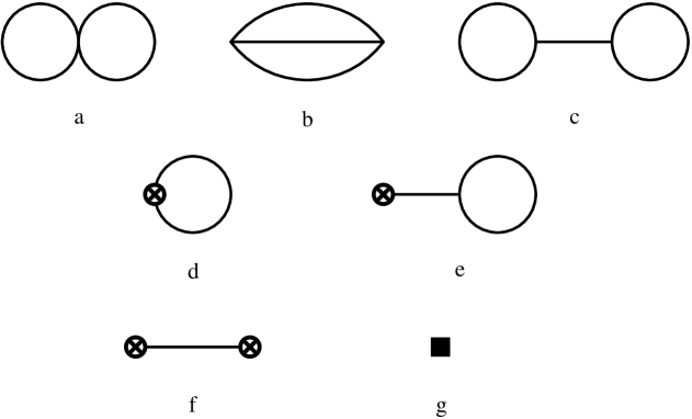
Figure 1: Skeleton diagrams for the generating functional $Z_{6}$ of $O(p^{6})$. Simple dots, crossed circles, black box denote vertices from LO, NLO, NNLO Lagrangians, respectively. Propagators and vertices carry the full tree structure associated with the lowest-order Lagrangian.

In Ref. [3], we proposed an analytic approximation for $Z_{6}$ of the following form:

$$Z_{6}^{I} = \int\!\!d^{4}x\left\{\left[C_{a}^{r}(\mu)+\displaystyle\frac{1}{4F_{0}^{2}}\left(4\,\Gamma_{a}^{(1)}\,L(\mu)-\Gamma_{a}^{(2)}\,L(\mu)^{2}+2\,\Gamma_{a}^{(L)}(\mu)L(\mu)\right)\right]O_{a}(x)\right.$$ (2.1)

$$+\left.\displaystyle\frac{1}{(4\pi)^{2}}\left[L_{i}^{r}(\mu)-\displaystyle\frac{\Gamma_{i}}{2}L(\mu)\right]H_{i}(x;M)\right\}$$

$$+ \int\!\!d^{4}x\,d^{4}y\left\{\left(L_{i}^{r}(\mu)-\displaystyle\frac{\Gamma_{i}}{2}L(\mu)\right)P_{i,\alpha}(x)\,G_{\alpha,\beta}(x,y)\left(L_{j}^{r}(\mu)-\displaystyle\frac{\Gamma_{j}}{2}L(\mu)\right)P_{j,\beta}(y)\right.$$

$$+\left.2\,\left(L_{i}^{r}(\mu)-\displaystyle\frac{\Gamma_{i}}{2}L(\mu)\right)P_{i,\alpha}(x)\,G_{\alpha,\beta}(x,y)\,F_{\beta}(y;M)\right\}~{}.$$

The monomials $O_{a}(x)~{}(a=1,\dots,94)$ define the chiral Lagrangian of $O(p^{6})$ [7] with associated renormalized LECs $C_{a}^{r}(\mu)$ and the $L_{i}^{r}(\mu)~{}(i=1,\dots,10)$ are renormalized LECs of $O(p^{4})$ with associated beta functions $\Gamma_{i}$ [6]. The coefficients $\Gamma_{a}^{(1)}$, $\Gamma_{a}^{(2)}$ and $\Gamma_{a}^{(L)}$ are listed in Ref. [4]. Repeated indices are to be summed over. $F_{0}$ is the meson decay constant in the chiral $SU(3)$ limit. The chiral log

$$L(\mu)=\displaystyle\frac{1}{(4\pi)^{2}}\ln{M^{2}/\mu^{2}}$$ (2.2)

involves an arbitrary scale $M$. This scale is introduced in the complete functional $Z_{6}$ in Eq. (A.21) to make the scale dependence explicit: only $C_{a}^{r}(\mu)$, $L_{i}^{r}(\mu)$ and $L(\mu)$ in (2.1) depend on the renormalization scale $\mu$. The various functionals in Eq. (2.1) are defined in App. A. The approximation consists in dropping in $Z_{6}$ the irreducible two-loop contributions represented by the functional $K(x;M)$ (diagrams a,b in Fig. 1) and the terms bilinear in $F_{\alpha}(x;M)$ (diagram c in Fig. 1), except for single and double logs.

The procedure how to actually calculate an amplitude corresponding to Eq. (2.1) was described in Ref.  [3]. In many cases, the relevant amplitudes can be extracted from available calculations of $O(p^{6})$ [2].

Approximation I defined by Eq. (2.1) has the following properties [3]:

• All chiral logs are included.

• The functional $Z_{6}^{I}$ is independent of the renormalization scale $\mu$. Unlike the double-log approximation[8], it therefore allows for the extraction of LECs with the correct scale dependence.

• In addition to single and double logs, the residual dependence on the scale $M$ is the only other vestige of the two-loop part.

• In dropping the genuine two-loop contributions, Approximation I respects the large-$N_{c}$ hierarchy of $O(p^{6})$ contributions:
                    $C_{a},L_{i}L_{j}\quad\longrightarrow\quad L_{i}\times$ loop $\quad\longrightarrow\quad$ two-loop contributions
  

• Only tree and one-loop amplitudes need to be calculated.

The question still remains to be answered how reliable this approximation is. We shall adopt the following criterion. For an $SU(3)$ quantity normalized to one at lowest order, successive terms in the chiral expansion usually show the following generic behaviour:

$O(p^{4})$	$O(p^{6})$	$O(p^{8})$
$\mathrel{\hbox to0.0pt{\lower 4.0pt\hbox{\hskip 1.0pt$\sim$}\hss}\raise 1.0pt\hbox{$<$}}0.3$	$\mathrel{\hbox to0.0pt{\lower 4.0pt\hbox{\hskip 1.0pt$\sim$}\hss}\raise 1.0pt\hbox{$<$}}0.3^{2}=0.09$	$\mathrel{\hbox to0.0pt{\lower 4.0pt\hbox{\hskip 1.0pt$\sim$}\hss}\raise 1.0pt\hbox{$<$}}0.3^{3}=0.027$

This suggests as a criterion for an acceptable NNLO approximation that the accuracy should not be worse than 3 $\%$, the typical size of contributions of $O(p^{8})$. As the following examples will show, the quality of the approximation depends on the scale $M$, which parametrizes the two-loop contributions not contained in (2.1). Although the acceptable range will depend on the quantity under consideration, experience with the double-log approximation [8] in chiral $SU(3)$ suggests that $M$ is of the order of $M_{K}$.

Approximation I is motivated by large $N_{c}$, but in some cases the accuracy may be improved by including in the approximate functional (2.1) also products of one-loop amplitudes (diagrams a,c in Fig. 1, subleading in $1/N_{c}$), which also have a simple analytic form. We call this extension Approximation II. In contrast to Approximation I, this extension is not uniquely defined because it depends on the representation of the matrix field $U$. In the standard representation used, e.g., also in Refs. [4, 9], it amounts to omitting (except for chiral logs) the sunset diagram b from the full functional $Z_{6}$ in Eq. (A.21).

3 $\mathbf{F_{K}/F_{\pi}}$ and the low-energy constant $\mathbf{L_{5}}$

The ratio of pseudoscalar decay constants $F_{K}/F_{\pi}$ appears well suited for our analytic approximations. The chiral expansion of $F_{K}/F_{\pi}-1$ is shown for physical meson masses in Table 1. The separately scale-dependent contributions of $O(p^{6})$ are given for the usual renormalization scale $\mu=770$ MeV. The entries for “numerical results” were provided by Bernard and Passemar [10].

	$O(p^{4})$		$O(p^{6})$
		2-loop	$L_{i}\times$ loop	tree
numerical results [9, 10]	0.14	0.002	0.051	0.008
Approximation I ($M=M_{K}$)		- 0.030
Approximation II ($M=M_{K}$)		- 0.011

Table 1: Chiral expansion of $F_{K}/F_{\pi}-1$. The separate contributions of $O(p^{6})$ are listed for $\mu=770$ MeV.

Figure 2: $M$-dependence of Approximations I, II for the two-loop contributions to $F_{K}/F_{\pi}$ at $\mu=770$ MeV. The blue bands denote the $\pm 3\%$ regions around the actual values provided by Bernard and Passemar [10]. The dashed black curves correspond to Approximation I, the dash-dotted red curves to Approximation II. The left panel describes the situation for physical meson masses, the right panel for masses $M_{\pi}=416$ MeV, $M_{K}=604$ MeV.

As shown in Table 1, Approximation I barely meets our criterion of acceptability put forward at the end of the last section, while Approximation II does much better. To investigate also the dependence on the scale $M$, we display in Fig. 2 the variation with $M$ for both versions I and II and for two sets of meson masses. As demonstrated in Fig. 2, there is little dependence on $M$ in the vicinity of $M=M_{K}$. Nevertheless, we will account for this variation in the final errors for the preferred Approximation II.

The explicit expression for Approximation II of $F_{K}/F_{\pi}$ is given in App. B where all masses are lowest-order masses of $O(p^{2})$. Since we work to $O(p^{6})$ the masses in $R_{4}$ must be expressed in terms of the lattice masses to $O(p^{4})$ [6]. The chiral limit value $F_{0}$ is expressed in terms of the experimental value $F_{\pi}=92.2$ MeV and physical meson masses, using again the $O(p^{4})$ relation. In $R_{6}$ and $R_{6}^{\rm ext}$, $F_{0}$ and the meson masses can be replaced by $F_{\pi}$ and lattice masses, respectively.

We now repeat the analysis of $F_{K}/F_{\pi}$ performed in Ref. [3] with Approximation II. We recall that at $O(p^{4})$ only the LEC $L_{5}$ enters. At $O(p^{6})$, two combinations of NNLO LECs appear: $C_{14}+C_{15}$ and $C_{15}+2C_{17}$. At this order, also some of the $L_{i}$ enter, but only the term with $L_{5}^{2}$ is leading in $1/N_{c}$. In the spirit of large $N_{c}$, we therefore extract as in Ref. [3] $L_{5}$, $C_{14}+C_{15}$ and $C_{15}+2C_{17}$ from a fit of the lattice data of the BMW Collaboration [11], using for the remaining $L_{i}$ (appearing only at $O(p^{6})$, subleading in $1/N_{c}$) the values of fit 10 of Ref. [12]. The results are displayed in Table 2.

	$F_{K}/F_{\pi}$	$10^{3}L_{5}^{r}$	$10^{3}(C_{14}^{r}+C_{15}^{r})$	$10^{3}(C_{15}^{r}+2C_{17}^{r})$
App. I ($M=M_{K}$)	$1.198(5)$	$0.76(8)$	$0.37(7)$	$1.29(14)$
App. II	$1.200(5)$	$0.75(8)$	$0.20(8)$	$0.71(22)$
BMW [11]	$1.192(7)_{\rm stat}(6)_{\rm syst}$

Table 2: Fit results for $F_{K}/F_{\pi}$ and LECs for Approximations I (statistical errors only) and II. The renormalization scale is $\mu=770$ MeV for all LECs. The LECs $C_{a}^{r}$ have dimension ${\rm GeV}^{-2}$.

The fitted values of $F_{K}/F_{\pi}$ agree with the detailed analysis of Ref. [11]. For both $F_{K}/F_{\pi}$ and $L_{5}$, there is practically no difference between the two approximations but the LECs of $O(p^{6})$ show a bigger spread. For Approximation II, we have added the uncertainty due to varying $M$ in the range $0.9\leq M/M_{K}\leq 1.1$ in quadrature to the statistical lattice errors. The effect of this variation is small, for $F_{K}/F_{\pi}$ and $L_{5}$ in fact negligible. Since $C_{15}$ is subleading in $1/N_{c}$ the fit determines essentially $C_{14}$ and $C_{17}$ [10]. Although the values depend of course on the input for the $L_{i}$, the results in Table 2 suggest that both $C_{14}^{r}$ and $C_{17}^{r}$ are positive and smaller than $10^{-3}~{}{\rm GeV}^{-2}$, always taken at $\mu=0.77$ GeV. We will use these fit results with Approximation II for $L_{5}^{r}$, $C_{14}^{r}$ and $C_{17}^{r}$ in the analysis of $F_{\pi}/F_{0}$ in the following section.

The fit also demonstrates very clearly that NNLO terms are essential. While the NNLO fit (Approximation II) is well behaved ($\chi^{2}$/dof = 1.2, statistical errors only), the NLO fit with the single parameter $L_{5}$ is unacceptable ($\chi^{2}$/dof = 4). Analysing present-day lattice data with NLO chiral $SU(3)$ expressions does not make sense.

4 $\mathbf{F_{\pi}}$ and the low-energy constants $\mathbf{F_{0},L_{4}}$

The meson decay constant in the chiral limit is a LEC of the lowest-order chiral Lagrangian. In the case of chiral $SU(2)$, $F=\lim_{m_{u},m_{d}\to 0}F_{\pi}$ is well known, mainly from a combined analysis of lattice data with $N_{f}=2$ active flavours by the FLAG Collaboration [1]:

$$F=(85.9\pm 0.6)~{}{\rm MeV}~{}.$$ (4.1)

The situation is quite different in the $SU(3)$ case. The lattice results for $F_{0}=\lim_{m_{u},m_{d},m_{s}\to 0}F_{\pi}$ cover a much wider range, from about 66 MeV to 84 MeV [1]. A similar range is covered in the phenomenological fits of Bijnens and Jemos [13].

The low-energy expansion in chiral $SU(3)$ is characterized by the ratio $p^{2}/(4\pi F_{0})^{2}$ where $p$ stands for a generic meson momentum or mass. $F_{0}$ thus sets the scale for the chiral expansion. In practice, $F_{0}$ is usually traded for $F_{\pi}$ at successive orders of the chiral expansion. Nevertheless, $F_{0}$ affects the “convergence” of the chiral expansion: a smaller $F_{0}$ tends to produce bigger fluctuations at higher orders.

Why has it been so difficult both for lattice and phenomenological studies to determine $F_{0}$? One clue is the apparent anti-correlation with the NLO LEC $L_{4}$ in the fits of Ref. [13]: the bigger $F_{0}$, the smaller $L_{4}^{r}(M_{\rho})$, and vice versa. The large-$N_{c}$ suppression of $L_{4}$ is not manifest in the fits with small $F_{0}$.

This anti-correlation can be understood to some extent from the structure of the chiral $SU(3)$ Lagrangian up to and including NLO:

$${\cal L}_{p^{2}}(2)+{\cal L}_{p^{4}}(10) = \displaystyle\frac{F_{0}^{2}}{4}\langle D_{\mu}UD^{\mu}U^{\dagger}+\chi U^{\dagger}+\chi^{\dagger}U\rangle+L_{4}\langle D_{\mu}UD^{\mu}U^{\dagger}\rangle\langle\chi U^{\dagger}+\chi^{\dagger}U\rangle+\dots$$ (4.2)

$$= \displaystyle\frac{1}{4}\langle D_{\mu}UD^{\mu}U^{\dagger}\rangle\left[F_{0}^{2}+8L_{4}\left(2\accentset{\circ}{M}^{2}_{K}+\accentset{\circ}{M}^{2}_{\pi}\right)\right]+\dots~{}$$

The unitary matrix field $U$ is parametrized by the meson fields, $\chi=2B_{0}{\cal M}_{q}$ ($B_{0}\sim$ quark condensate, ${\cal M}_{q}$ is the quark mass matrix), $\langle\dots\rangle$ stands for the $SU(3)$ flavour trace and $\accentset{\circ}{M}_{P}$ denotes the lowest-order meson masses. The dots refer to the remainder of the NLO Lagrangian in the first line and to terms of higher order in the meson fields in the second line. Therefore, a LO tree-level contribution is always accompanied by an $L_{4}$ contribution in the combination

$$F(\mu)^{2}:=F_{0}^{2}+8L_{4}^{r}(\mu)\left(2\accentset{\circ}{M}^{2}_{K}+\accentset{\circ}{M}^{2}_{\pi}\right)~{}.$$ (4.3)

Of course, there will in general be additional contributions involving $L_{4}$ at NLO, especially in higher-point functions (e.g., in meson meson scattering). Nevertheless, the observed anti-correlation between $F_{0}$ and $L_{4}$ is clearly related to the structure of the chiral Lagrangian. Note that $F^{2}_{\pi}/16M_{K}^{2}=2\times 10^{-3}$ is the typical size of a NLO LEC. Although of different chiral order, the two terms in $F(\mu)^{2}$ could a priori be of the same order of magnitude.

Independent information on $F_{0}$ comes from comparing the $SU(2)$ and $SU(3)$ expressions for $F_{\pi}$. To $O(p^{4})$ in chiral $SU(2)$, $F_{\pi}$ is given by [5]

$$F_{\pi}=F+F^{-1}\left[M_{\pi}^{2}\,l_{4}^{r}(\mu)+\overline{A}(M_{\pi},\mu)\right]$$ (4.4)

where $l_{4}$ is a NLO $SU(2)$ LEC and $\overline{A}(M_{\pi},\mu)$ is a one-loop function defined in Eq. (B.5). Expressing $l_{4}^{r}(\mu)$ in terms of $L_{4}^{r}(\mu)$, $L_{5}^{r}(\mu)$ and a kaon loop contribution [6] and equating Eq. (4.4) with the $SU(3)$ result for $F_{\pi}$, one arrives at the following relation:

$$F_{0} = F-F^{-1}\left\{\left(2M_{K}^{2}-M_{\pi}^{2}\right)\left(4L_{4}^{r}(\mu)+\displaystyle\frac{1}{64\pi^{2}}\ln{\displaystyle\frac{\mu^{2}}{M_{K}^{2}}}\right)+\displaystyle\frac{M_{\pi}^{2}}{64\pi^{2}}\right\}+O(p^{6})~{}.$$ (4.5)

To $O(p^{6})$, the relation between $F_{0}$ and $F$ was derived by Gasser et al. [14]. It depends on LECs of both NLO and NNLO. In Fig. 4, both $O(p^{4})$ and $O(p^{6})$ relations will be displayed. Of course, in order to plot $F_{0}$ as a function of $L_{4}$ to $O(p^{6})$, some assumptions about NLO and NNLO LECs are needed.

$SU(3)$ lattice data for $F_{\pi}$ seem well suited for a determination of $F_{0}$ and $L_{4}$ although the emphasis in most lattice studies has been to determine $F_{\pi}$ itself. As for $F_{K}/F_{\pi}$, the use of CHPT to NNLO, $O(p^{6})$ [9], is essential for a quantitative analysis.

In the following, we are going to apply Approximation I for the analysis of $F_{\pi}$. It turns out that, unlike for $F_{K}/F_{\pi}$, Approximation I agrees better with the numerical results of Ref. [10] than Approximation II. The explicit representation for $F_{\pi}$ is given in App. C. The lowest-order masses appearing in the terms of $O(p^{4})$ must again be expressed in terms of lattice masses. Unlike in the previous section, we leave $F_{0}$ in Eq. (C.1) untouched.

Again in contrast to the ratio $F_{K}/F_{\pi}$, the dependence on the mass parameter $M$ is more pronounced in this case, especially for larger meson masses (see Fig. 3). To satisfy the requirement that our approximation should stay within $\pm 3\%$ of the exact numerical results [10], we are going to vary $M$ in the range $0.97\leq M/M_{K}\leq 1.09$.

Figure 3: $M$-dependence of Approximation I for the two-loop contributions to $F_{\pi}$ at $\mu=770$ MeV (dashed black curves). The blue bands denote the $\pm 3\%$ regions around the actual values provided by Bernard and Passemar [10]. The left panel describes the situation for physical meson masses, the right panel for masses $M_{\pi}=416$ MeV, $M_{K}=604$ MeV.

In addition to $F_{0}$ and $L_{4}$, the only other LEC appearing to $O(p^{4})$ in Eq. (C.1) is $L_{5}$. On the basis of the analysis of $F_{K}/F_{\pi}$ in Sec. 3, we will use $L_{5}^{r}=(0.75\pm 0.10)\cdot 10^{-3}$. At $O(p^{6})$, the following NNLO LECs enter: $C_{14}$, $C_{15}$, $C_{16}$ and $C_{17}$, but only $C_{14}$ and $C_{17}$ are leading in $1/N_{c}$. In the spirit of large $N_{c}$, we therefore use the values for $C_{14}$ and $C_{17}$ obtained in the previous section, neglecting at the same time $C_{15}$ and $C_{16}$. However, we assign a 100 $\%$ uncertainty to both $C_{14}$ and $C_{17}$. Anticipating the dependence of the relation between $F_{0}$ and $F$ at $O(p^{6})$ on $C_{16}$ [14] in Fig. 4, we include for consistency the uncertainty due to varying $C^{r}_{16}(M_{\rho})$ between $\pm C^{r}_{14}(M_{\rho})$. At $O(p^{6})$, some more of the NLO LECs $L_{i}$ enter. For definiteness, we use again fit 10 of Ref. [12] for those LECs. However, any other set of values for the $L_{i}$ from Refs. [12, 13] consistent with large $N_{c}$, in particular with a small $L_{4}^{r}(M_{\rho})$, leads to very similar results.

We confront the expression (C.1) for $F_{\pi}$ with lattice data from the RBC/UKQCD Collaboration [15, 16]. In our main fit we only consider (five) unitary lattice points with $M_{\pi}<350$ MeV. In this case, $F_{\pi}$ for physical meson masses emerges as a fit result but the fitted value is lower than the experimental value. Another alternative is therefore to use in addition to the lattice points also the experimental value $F_{\pi}=(92.2\pm 0.3)$ MeV as input where we have doubled the error assigned by the Particle Data Group [17].

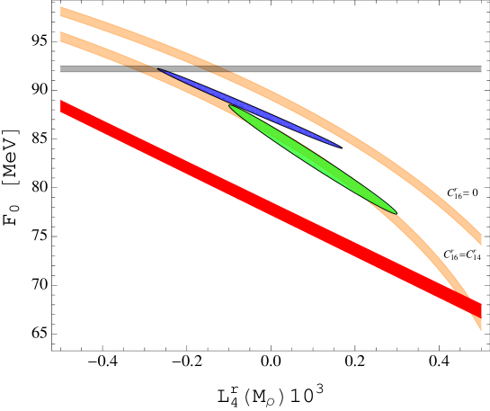
Figure 4: Fitted values of $F_{0}$, $L_{4}$ using RBC/UKQCD data [15, 16] with $M_{\pi}<350$ MeV, with (blue ellipse) and without (green ellipse) including $F_{\pi}^{\rm phys}$. The red band results from the comparison of $F_{\pi}$ between $SU(2)$ and $SU(3)$ as expressed by Eq. (4.5), taking $F=(85.9\pm 0.6)~{}{\rm MeV}$ [1]. The relation between $F_{0}$ and $F$ to $O(p^{6})$ [14] leads to the orange bands for two values of $C^{r}_{16}(M_{\rho})$. The horizontal grey band denotes $F_{\pi}=(92.2\pm 0.3)$ MeV.

The extracted values of $F_{0}$ and $L_{4}^{r}(M_{\rho})$ are shown in Fig. 4. For the case where $F_{\pi}^{\rm phys}$ is included (blue ellipse), the explicit fit results are:

$$F_{0} = (88.1\pm 4.1)~{}{\rm MeV}$$

$$10^{3}L_{4}^{r}(M_{\rho}) = -0.05\pm 0.22$$

$${\rm corr}(F_{0},L_{4}^{r}) = -0.996~{}.$$ (4.6)

The errors of $F_{0}$, $L_{4}$ are due to both lattice and theoretical uncertainties. First, there are statistical errors of the lattice values for $F_{\pi}$ and the meson masses and, in addition, the uncertainties of the inverse lattice spacings. The dominant errors are those of the lattice spacings and of $F_{\pi}$, whereas the errors of the lattice masses are practically negligible. We have neglected unknown correlations among the lattice data, thereby probably overestimating the combined errors.

In addition, we added the theoretical uncertainties related to $M$, $L_{5}$ and the $C_{a}$ in quadrature. Lattice and theoretical errors are of similar size. For instance, keeping only the lattice errors, the error of $F_{0}$ moves from $4.1$ down to $2.8$ MeV. The $\chi^{2}/$dof is 0.5 (statistical errors only), suggesting once more that we have at least not underestimated the errors.

The two ellipses are roughly compatible with each other. The green ellipse is lower because from the RBC/UKQCD data alone the fitted value of $F_{\pi}$ is smaller than the experimental value. The value for $L_{4}$ is consistent with large $N_{c}$ and with available lattice results [1]. The result for $F_{0}$ is more precise than existing phenomenological and lattice determinations. It is somewhat bigger than expected [18], roughly of the same size as the $SU(2)$ LEC $F$ in Eq. (4.1).

$F_{0}$ and $L_{4}$ in Eq. (4.6) are compatible with the comparison between $SU(2)$ and $SU(3)$ to $O(p^{6})$ [14], as indicated by the orange bands in Fig. 4. $C_{16}$ is the only NNLO LEC appearing in the relation between $F_{0}$ and $F$. As always in this paper, we have used fit 10 [12] for the NLO LECs. However, unlike for our fit results (4.6), the orange bands in Fig. 4 are rather sensitive to the precise values of the $L^{r}_{i}$. Therefore, although the consistency between the ellipses and the lower orange band is manifest, it can hardly be used as a determination of $C_{16}$.

Raising the range in pion masses to $M_{\pi}<425$ MeV, two more lattice points [15] can be added. Repeating the fit with the bigger sample moves the ellipses down, because with the original data set of RBC/UKQCD the fitted value of $F_{\pi}$ comes out too low [15].

The strong anti-correlation between $F_{0}$ and $L_{4}$ persists because the kaon masses in the RBC/UKQCD data are all close to the physical kaon mass. Simulations with smaller kaon masses would not only be welcome from the point of view of convergence of the chiral series [19], but they could also provide a better lever arm for reducing the anti-correlation and the fit errors of $F_{0}$ and $L_{4}$. This expectation is supported by the fact that the quantity $F(M_{\rho})$ defined in Eq. (4.3) can be determined much better than $F_{0}$.

5 Remarks on $\mathbf{f^{K\pi}_{+}(0)}$

The kaon semileptonic vector form factor at $t=0$ is a crucial quantity for a precision determination of the CKM matrix element $V_{us}$. Both approximations discussed here do not appear very promising in this case.

First of all, unlike for $F_{\pi}$ and $F_{K}/F_{\pi}$, the chiral expansion of $f^{K\pi}_{+}(0)$ shows a rather atypical behaviour. Due to the Ademollo-Gatto theorem [20], the $O(p^{4})$ contribution of $-0.0227$ [21] is very small. On the basis of recent lattice studies, which find $f^{K\pi}_{+}(0)=0.967$ with errors of less than $1\%$ [22, 23], all higher-order contributions in CHPT would have to sum up to about $-1\%$. On the other hand, the genuine two-loop contributions at the usual scale $\mu=770$ MeV are positive and slightly bigger than $1\%$ [24, 25, 10], suggesting that the remainder is about $-2\%$ to match the lattice value. In other words, the remainder would have to be as big as the NLO contribution, certainly not the typical behaviour for a chiral expansion.

In principle, Approximation I fulfills our criterion of Sec. 2 in differing from the full two-loop result [24, 25, 10] by less than $2\%$. However, especially in view of the accuracy of recent lattice studies claiming a precision of better than $1\%$ for $f^{K\pi}_{+}(0)$, the accuracy of Approximation I is simply not sufficient in this case. Approximation II does not improve the situation.

To sum up, lattice determinations of $f^{K\pi}_{+}(0)$ seem to be able to do without CHPT. Moreover, only the full NNLO expression may allow for a meaningful extraction of LECs if at all [10].

6 Conclusions

We summarize the main results of our work.

1. Lattice QCD has become a major source of information for the low-energy constants of CHPT. We have argued that the meson decay constants $F_{\pi}$, $F_{K}$ are especially suited for extracting chiral $SU(3)$ LECs of different chiral orders. The ratio $F_{K}/F_{\pi}$ allows for a precise and stable determination of the NLO LEC $L_{5}$. In addition, it gives access to some NNLO LECs although the accuracy is of course more limited in that case. Phenomenological analyses have had difficulties in determining the LEC $F_{0}$, the meson decay constant in the chiral $SU(3)$ limit. We have shown that lattice data for $F_{\pi}$ allow for the extraction of $F_{0}$ together with the NLO LEC $L_{4}$. The strong anti-correlation between $F_{0}$ and $L_{4}$ observed in phenomenological analyses can in principle be lifted by varying the lattice masses. From a fit to the RBC/UKQCD data for $F_{\pi}$, we have obtained a value for $F_{0}$ that is more precise than other presently available determinations.

2. Confronting present-day lattice data with chiral $SU(3)$ requires chiral amplitudes to NNLO in most cases. Chiral $SU(3)$ amplitudes are often rather unwieldy and mostly available in numerical form only. We have therefore proposed large-$N_{c}$ motivated approximate NNLO amplitudes that contain only one-loop functions. Unlike simpler approximations as the double-log approximation, our amplitudes are independent of the renormalization scale and can therefore be used to extract LECs with the correct scale dependence. However, approximations of NNLO amplitudes can only be successful if the differences to the full amplitudes are at most of the order of N³LO contributions. We have checked that this criterion can be fulfilled with our approximate amplitudes both for $F_{\pi}$ and $F_{K}/F_{\pi}$. Therefore, we expect our results for the different LECs to be as reliable as CHPT to NNLO, $O(p^{6})$, permits. Although our general criterion is also satisfied for the kaon semileptonic form factor at $t=0$, the approximate expression for $f^{K\pi}_{+}(0)$ is not precise enough compared to recent lattice data.

The main purpose of this work has been to encourage lattice groups to use NNLO amplitudes in chiral $SU(3)$ that are more user friendly than the full expressions and yet are reliable enough to provide more insight than NLO amplitudes with polynomial corrections.

Acknowledgements

We are grateful to Véronique Bernard, Claude Bernard, Gilberto Colangelo, Laurent Lellouch, Heiri Leutwyler, Emilie Passemar and Lothar Tiator for helpful comments and suggestions. We are indebted to Elvira Gámiz for helping us to understand lattice data. Special thanks are due to Hans Bijnens for suggesting several substantial improvements of the original manuscript and for making the full results of Ref. [9] accessible to us. P.M. acknowledges support from the Deutsche Forschungsgemeinschaft DFG through the Collaborative Research Center “The Low-Energy Frontier of the Standard Model” (SFB 1044).

Appendix A Generating functional of $\mathbf{O(p^{6})}$

In this appendix we rederive the generating functional of $O(p^{6})$ in the form used in Ref. [3]. It is a more explicit version of the derivation in Ref. [4].

The generating functional $Z_{6}$ is shown pictorially in Fig. 1. The various contributions to $Z_{6}$ are always understood as functionals of the classical field, the solution of the lowest-order field equations.

As discussed in Ref. [4], the sum of the reducible diagrams c, e, f leads to a finite and scale independent functional with the conventional choice of chiral Lagrangians. The contributions from diagrams a, b and d are divergent. The sum $Z_{6}^{\rm a+b+d}$ is still divergent, but the divergence takes the form of a local functional that is canceled by the divergent part of the tree-level functional $Z_{6}^{\rm g}$ in terms of the LECs $C_{a}$ of $O(p^{6})$.

We first consider the irreducible two-loop diagrams a, b. In d dimensions, the corresponding functional has the form

$$Z_{6}^{\rm a+b} = \int\!\!d^{d}x(c\mu)^{2(d-4)}\left\{\Lambda^{2}\sum_{a}\alpha_{a}O_{a}(x)+\displaystyle\frac{\Lambda}{(4\pi)^{2}}\left[\sum_{a}\left(\beta_{a}+\alpha_{a}\ln{M^{2}/\mu^{2}}\right)O_{a}(x)+D(x;M)\right]\right.$$ (A.1)

$$+\left.\displaystyle\frac{1}{(4\pi)^{4}}\left[E(x;M)+\ln^{2}{M^{2}/\mu^{2}}\sum_{a}\displaystyle\frac{\alpha_{a}}{2}O_{a}(x)+\ln{M^{2}/\mu^{2}}\left(\sum_{a}\beta_{a}O_{a}(x)+D(x;M)\right)\right]\right\}$$

with the divergence factor

$$\Lambda=\dfrac{1}{(4\pi)^{2}(d-4)}~{}.$$ (A.2)

The monomials $O_{a}(x)~{}(a=1,\dots,94)$ define the chiral $SU(3)$ Lagrangian of $O(p^{6})$ [7]. $D(x;M)$ and $E(x;M)$ are nonlocal functionals. The mass $M$ is introduced to make the dependence on the renormalization scale $\mu$ explicit. At this stage, the functional $Z_{6}^{\rm a+b}$ is independent of $M$. The scheme dependent constant $c$ is conventionally chosen as in Eq. (2.22) of Ref. [4]. Eq. (A.1) is equivalent to Eq. (2.39) in Ref. [4] but the renormalization group equations (2.40) [4] have already been taken into account. In other words, the scale independence of $Z_{6}^{\rm a+b}$ is made explicit implying

$$\mu\displaystyle\frac{\partial\alpha_{a}}{\partial\mu}=0~{},\qquad \qquad\mu\displaystyle\frac{\partial\beta_{a}}{\partial\mu}=0$$

$$\mu\displaystyle\frac{\partial D(x;M)}{\partial\mu}=0~{},\qquad \qquad\mu\displaystyle\frac{\partial E(x;M)}{\partial\mu}=0~{}.$$ (A.3)

The general structure of the irreducible one-loop functional d is

$$Z_{6}^{\rm d}=\int\!\!d^{d}x(c\mu)^{(d-4)}\sum_{i=1}^{10}L_{i}(d)Y_{i}(x,d)$$ (A.4)

where the LECs of $O(p^{4})$ are decomposed as

$$L_{i}(d)=(c\mu)^{d-4}\left[\Gamma_{i}\Lambda+L_{i}^{r}(\mu,d)\right]~{}.$$ (A.5)

Adopting the renormalization conventions of Ref. [4], the LECs $L_{i}^{r}(\mu,d)$ are not expanded around $d=4$. Scale independence of the $L_{i}(d)$ then implies

$$\mu\displaystyle\frac{\partial L_{i}^{r}(\mu,d)}{\partial\mu}=-\displaystyle\frac{\Gamma_{i}}{(4\pi)^{2}}-(d-4)L_{i}^{r}(\mu,d)~{}.$$ (A.6)

Because of the divergence in $L_{i}(d)$ one must keep track of terms of $O(d-4)$ in $Y_{i}(x,d)$. With hindsight, these functionals can be written as

$$Y_{i}(x,d) = \left(\Lambda+\displaystyle\frac{1}{2(4\pi)^{2}}\ln{M^{2}/\mu^{2}}\right)\sum_{a}\eta_{a}^{i}O_{a}(x)$$

$$+\displaystyle\frac{1}{(4\pi)^{2}}\left\{H_{i}(x,d;M)+(d-4)\left[\displaystyle\frac{1}{8}\ln^{2}{M^{2}/\mu^{2}}\sum_{a}\eta_{a}^{i}O_{a}(x)+\displaystyle\frac{1}{2}\ln{M^{2}/\mu^{2}}~{}H_{i}(x,d;M)\right]\right\}~{}.$$

The scale independence of $(c\mu)^{d-4}\,Y_{i}(x,d)$ implies that the coefficients $\eta_{a}^{i}$ are scale independent and that the functionals $H_{i}(x,d;M)$ satisfy the renormalization group equations

$$\mu\displaystyle\frac{\partial H_{i}(x,d)}{\partial\mu}=O[(d-4)^{2}]~{}.$$ (A.8)

Putting everything together, we obtain (using for convenience from now on the summation convention for both indices a, i)

$$Z_{6}^{\rm d} = \int\!\!d^{d}x(c\mu)^{2(d-4)}\left\{\Lambda^{2}\,\Gamma_{i}\eta_{a}^{i}O_{a}(x)\right.$$

$$+\displaystyle\frac{\Lambda}{(4\pi)^{2}}\left[(4\pi)^{2}L_{i}^{r}(\mu,d)\,\eta_{a}^{i}O_{a}(x)+\displaystyle\frac{1}{2}\ln{M^{2}/\mu^{2}}\,\Gamma_{i}\eta_{a}^{i}O_{a}(x)+\Gamma_{i}H_{i}(x,d;M)\right]$$

$$+\left.\displaystyle\frac{1}{(4\pi)^{4}}\left[\displaystyle\frac{1}{8}\ln^{2}{M^{2}/\mu^{2}}\,\Gamma_{i}\eta_{a}^{i}O_{a}(x)+\displaystyle\frac{1}{2}\ln{M^{2}/\mu^{2}}\,\Gamma_{i}H_{i}(x,4;M)\right.\right.$$

$$+\left.\left.\displaystyle\frac{1}{2}\ln{M^{2}/\mu^{2}}\,(4\pi)^{2}L_{i}^{r}(\mu,4)\eta_{a}^{i}O_{a}(x)+(4\pi)^{2}L_{i}^{r}(\mu,4)H_{i}(x,4;M)\right]+O(d-4)\right\}~{}.$$

Altogether, the irreducible contributions sum up to the functional

$$Z_{6}^{\rm a+b+d} = \int\!\!d^{d}x(c\mu)^{2(d-4)}\left\{\Lambda^{2}\left[\alpha_{a}+\Gamma_{i}\eta_{a}^{i}\right]O_{a}(x)\right.$$

$$+\displaystyle\frac{\Lambda}{(4\pi)^{2}}\left[\beta_{a}O_{a}(x)+\ln{M^{2}/\mu^{2}}\left(\alpha_{a}+\displaystyle\frac{1}{2}\Gamma_{i}\eta_{a}^{i}\right)O_{a}(x)\right.$$

$$+\left.D(x;M)+\Gamma_{i}H_{i}(x,d;M)+(4\pi)^{2}L_{i}^{r}(\mu,d)\,\eta_{a}^{i}O_{a}(x)\right]$$

$$+\displaystyle\frac{1}{(4\pi)^{4}}\left[E(x;M)+\ln^{2}{M^{2}/\mu^{2}}\,\displaystyle\frac{\alpha_{a}}{2}O_{a}(x)+\ln{M^{2}/\mu^{2}}\left(\beta_{a}O_{a}(x)+D(x;M)\right)\right.$$

$$+\displaystyle\frac{1}{8}\ln^{2}{M^{2}/\mu^{2}}\,\Gamma_{i}\eta_{a}^{i}O_{a}(x)+\displaystyle\frac{1}{2}\ln{M^{2}/\mu^{2}}\,\Gamma_{i}H_{i}(x,4;M)$$

$$+\left.\left.\displaystyle\frac{1}{2}\ln{M^{2}/\mu^{2}}\,(4\pi)^{2}L_{i}^{r}(\mu,4)\eta_{a}^{i}O_{a}(x)+(4\pi)^{2}L_{i}^{r}(\mu,4)H_{i}(x,4;M)\right]+O(d-4)\right\}\,.$$

The double-pole divergence functional is automatically local. In order to cancel the divergences with the local functional $Z_{6}^{\rm g}$, also the single-pole divergences in (A) must be local. Absence of the logarithmic terms implies the 94 Weinberg conditions [26]

$$\alpha_{a}=-\displaystyle\frac{1}{2}\Gamma_{i}\eta_{a}^{i}~{}.$$ (A.11)

Moreover, the non-local functional $D(x;M)$ must be canceled by $\Gamma_{i}H_{i}(x,4;M)$. More precisely, renormalization theory requires that

$$D(x;M)+\Gamma_{i}H_{i}(x,4;M)=\Delta\beta_{a}\,O_{a}(x)~{},$$ (A.12)

i.e., that the sum of the two terms is local. In Ref. [4] it was found that the cancellation is complete: $\Delta\beta_{a}=0$.

Using Eqs. (A.11) and (A.12) (with $\Delta\beta_{a}=0$), the irreducible functional is given by

$$Z_{6}^{\rm a+b+d} = \int\!\!d^{d}x(c\mu)^{2(d-4)}\left\{\displaystyle\frac{\Lambda^{2}}{2}\Gamma_{i}\eta_{a}^{i}O_{a}(x)+\displaystyle\frac{\Lambda}{(4\pi)^{2}}\left[\beta_{a}O_{a}(x)+(4\pi)^{2}L_{i}^{r}(\mu,d)\,\eta_{a}^{i}O_{a}(x)\right]\right.$$ (A.13)

$$+\displaystyle\frac{1}{(4\pi)^{4}}\left[-\displaystyle\frac{1}{8}\ln^{2}{M^{2}/\mu^{2}}\,\Gamma_{i}\eta_{a}^{i}O_{a}(x)+\displaystyle\frac{1}{2}\ln{M^{2}/\mu^{2}}\,(4\pi)^{2}L_{i}^{r}(\mu,4)\eta_{a}^{i}O_{a}(x)\right.$$

$$+\ln{M^{2}/\mu^{2}}\,\beta_{a}O_{a}(x)+H_{i}(x,4;M)\left((4\pi)^{2}L_{i}^{r}(\mu,4)-\displaystyle\frac{\Gamma_{i}}{2}\ln{M^{2}/\mu^{2}}\right)$$

$$+\left.\left.E(x;M)+\Gamma_{i}H_{i}^{\prime}(x,4;M)\right]+O(d-4)\right\}~{}.$$

The functional $H_{i}^{\prime}(x,4;M)$ is defined by the Taylor expansion

$$H_{i}(x,d;M)=H_{i}(x,4;M)+(d-4)H_{i}^{\prime}(x,4;M)+O[(d-4)^{2}]$$ (A.14)

and it is scale independent because of Eq. (A.8).

Now we can render the complete functional finite by adding the tree-level functional of $O(p^{6})$ (in the notation of Eq. (4.9) in Ref. [4]):

$$Z_{6}^{\rm g} = \int\!\!d^{d}x\,C_{a}(d)O_{a}(x)$$

$$= \int\!\!d^{d}x(c\mu)^{2(d-4)}\left[C_{a}^{r}(\mu,d)-\displaystyle\frac{\Gamma_{a}^{(2)}}{F^{2}}\Lambda^{2}-\displaystyle\frac{1}{F^{2}}\left(\Gamma_{a}^{(1)}+\Gamma_{a}^{(L)}(\mu,d)\right)\Lambda\right]O_{a}(x)~{}.$$

Comparing Eqs. (A.13) and (A), the divergences are canceled with

$$\Gamma_{a}^{(2)}=\displaystyle\frac{F^{2}}{2}\Gamma_{i}\eta_{a}^{i}~{},\qquad \Gamma_{a}^{(1)}=\displaystyle\frac{F^{2}}{(4\pi)^{2}}\beta_{a}~{},\qquad \Gamma_{a}^{(L)}(\mu,d)=F^{2}\,L_{i}^{r}(\mu,d)\,\eta_{a}^{i}~{}.$$ (A.16)

The coefficients $\Gamma_{a}^{(1)},\,\Gamma_{a}^{(2)},\,\Gamma_{a}^{(L)}(\mu,d)$ are listed in Table II of App. C in Ref. [4].

Summing up the diagrams a, b, d and g, the limit $d\to 4$ can now be taken to arrive at the final result

$$Z_{6}^{\rm a+b+d+g} = \int\!\!d^{4}x\left\{C_{a}^{r}(\mu)O_{a}(x)+\displaystyle\frac{1}{4F^{2}}\left(4\,\Gamma_{a}^{(1)}\,L(\mu)-\Gamma_{a}^{(2)}\,L^{2}(\mu)+2\,\Gamma_{a}^{(L)}(\mu)L(\mu)\right)O_{a}(x)\right.$$ (A.17)

$$+\left.\displaystyle\frac{1}{(4\pi)^{2}}\left[L_{i}^{r}(\mu)-\displaystyle\frac{\Gamma_{i}}{2}L(\mu)\right]H_{i}(x;M)+\displaystyle\frac{1}{(4\pi)^{4}}K(x;M)\right\}$$

with the chiral log $L(\mu)$ defined in Eq. (2.2) and with

$$C_{a}^{r}(\mu)=C_{a}^{r}(\mu,4)~{},\quad L_{i}^{r}(\mu)=L_{i}^{r}(\mu,4)~{},\quad\Gamma_{a}^{(L)}(\mu)=\Gamma_{a}^{(L)}(\mu,4)$$

$$\quad H_{i}(x;M)=H_{i}(x,4;M),\quad K(x;M)=E(x;M)+\Gamma_{i}H_{i}^{\prime}(x,4;M)~{}.$$ (A.18)

The scale dependence is contained in $C_{a}^{r}(\mu),\,L_{i}^{r}(\mu),\,L(\mu)$. The functionals $O_{a}(x)$, $H_{i}(x;M)$ and $K(x;M)$ are independent of $\mu$. Scale independence of the complete functional (A.17) can be checked with the help of the renormalization group equations (4.5) in Ref. [4]:

$$\mu\displaystyle\frac{dC_{a}^{r}(\mu)}{d\mu}=\displaystyle\frac{1}{(4\pi)^{2}F^{2}}\left[2\Gamma^{(1)}_{a}+\Gamma^{(L)}_{a}(\mu)\right]~{}.$$ (A.19)

As already mentioned, the sum of reducible diagrams c, e, f is finite and scale independent by itself. It can be written in the form

$$Z_{6}^{\rm c+e+f} = \int\!\!d^{4}x\,d^{4}y\left[\left(L_{i}^{r}(\mu)-\displaystyle\frac{\Gamma_{i}}{2}L(\mu)\right)P_{i,\alpha}(x)+F_{\alpha}(x;M)\right]G_{\alpha,\beta}(x,y)$$ (A.20)

$$\times\left[\left(L_{j}^{r}(\mu)-\displaystyle\frac{\Gamma_{j}}{2}L(\mu)\right)P_{j,\beta}(y)+F_{\beta}(y;M)\right]~{}.$$

The derivatives of the monomials $P_{i}(x)$ defining the chiral Lagrangian of $O(p^{4})$ with respect to the fields $\varphi_{\alpha}$ ($\alpha=1,\dots,8$) are denoted $P_{i,\alpha}(x)$. The $F_{\alpha}(x;M)$ are finite and scale independent one-loop functionals. The propagator $G_{\alpha,\beta}(x,y)$ is again a functional of the classical field. Although the functional (A.20) is nonlocal in general, it contributes in many cases of interest to wave function, mass and decay constant renormalization only.

The complete generating functional of $O(p^{6})$ is then given by the sum

$$Z_{6}=Z_{6}^{\rm a+b+d+g}+Z_{6}^{\rm c+e+f}~{}.$$ (A.21)

Once again, it is independent of both scales $\mu$ and $M$.

Appendix B Approximation II for $\mathbf{F_{K}/F_{\pi}}$

The original Approximation I for $F_{K}/F_{\pi}$ was given in the appendix of Ref. [3]. In Approximation II discussed in Sec. 3, there is an additional contribution of $O(p^{6})$ denoted $R_{6}^{\rm ext}$ below. The complete result for $F_{K}/F_{\pi}$ is

$$F_{K}/F_{\pi} = 1+R_{4}+R_{6}+R_{6}^{\rm ext}~{},$$ (B.1)

$$F_{0}^{2}\,R_{4} = 4\,(\accentset{\circ}{M}_{K}^{2}-\accentset{\circ}{M}_{\pi}^{2})\,L_{5}-5\,\overline{A}(\accentset{\circ}{M}_{\pi},\mu)/8+\overline{A}(\accentset{\circ}{M}_{K},\mu)/4+3\,\overline{A}(\accentset{\circ}{M}_{\eta},\mu)/8~{},$$ (B.2)

$$F_{0}^{4}\,R_{6} = 8\,F_{0}^{2}(\accentset{\circ}{M}_{K}^{2}-\accentset{\circ}{M}_{\pi}^{2})\left(2\,\accentset{\circ}{M}_{K}^{2}\,(C_{14}+C_{15})+\accentset{\circ}{M}_{\pi}^{2}\,(C_{15}+2\,C_{17})\right)$$ (B.3)

$$+ (\accentset{\circ}{M}_{K}^{2}-\accentset{\circ}{M}_{\pi}^{2})\,\left(-32\,(\accentset{\circ}{M}_{\pi}^{2}+2\,\accentset{\circ}{M}_{K}^{2})L_{4}\,L_{5}-8\,(3\,\accentset{\circ}{M}_{\pi}^{2}+\accentset{\circ}{M}_{K}^{2})L_{5}^{2}\right.$$

$$+\left.(25\,\accentset{\circ}{M}_{\pi}^{2}+17\,\accentset{\circ}{M}_{K}^{2})L^{2}/32\right)$$

$$+ \displaystyle\frac{(\accentset{\circ}{M}_{K}^{2}-\accentset{\circ}{M}_{\pi}^{2})}{(4\pi)^{2}}\left(-2\,(\accentset{\circ}{M}_{\pi}^{2}+\accentset{\circ}{M}_{K}^{2})L_{1}-(\accentset{\circ}{M}_{\pi}^{2}+\accentset{\circ}{M}_{K}^{2})L_{2}-(5\,\accentset{\circ}{M}_{\pi}^{2}+\accentset{\circ}{M}_{K}^{2})L_{3}/18\right.$$

$$+\left.6\,(\accentset{\circ}{M}_{\pi}^{2}+2\,\accentset{\circ}{M}_{K}^{2})L_{4}+(14\,\accentset{\circ}{M}_{\pi}^{2}+22\,\accentset{\circ}{M}_{K}^{2})L_{5}/3-12\,(\accentset{\circ}{M}_{\pi}^{2}+2\,\accentset{\circ}{M}_{K}^{2})L_{6}\right.$$

$$+\left.16\,(\accentset{\circ}{M}_{\pi}^{2}-\accentset{\circ}{M}_{K}^{2})L_{7}-4\,(\accentset{\circ}{M}_{\pi}^{2}+5\,\accentset{\circ}{M}_{K}^{2})L_{8}+(313\,\accentset{\circ}{M}_{\pi}^{2}+271\,\accentset{\circ}{M}_{K}^{2})L/288\right)$$

$$+ 5\,\overline{A}(\accentset{\circ}{M}_{\pi},\mu)^{2}/8-\overline{A}(\accentset{\circ}{M}_{K},\mu)^{2}/8+\overline{A}(\accentset{\circ}{M}_{\pi},\mu)\,\overline{A}(\accentset{\circ}{M}_{K},\mu)/16$$

$$- 3\,\overline{A}(\accentset{\circ}{M}_{\pi},\mu)\,\overline{A}(\accentset{\circ}{M}_{\eta},\mu)/8-3\,\overline{A}(\accentset{\circ}{M}_{K},\mu)\,\overline{A}(\accentset{\circ}{M}_{\eta},\mu)/16$$

$$+ \overline{A}(\accentset{\circ}{M}_{\pi},\mu)\left(4\,\accentset{\circ}{M}_{\pi}^{2}L_{1}+10\,\accentset{\circ}{M}_{\pi}^{2}L_{2}+13\,\accentset{\circ}{M}_{\pi}^{2}L_{3}/2+10\,(\accentset{\circ}{M}_{\pi}^{2}+2\,\accentset{\circ}{M}_{K}^{2})L_{4}\right.$$

$$+\left.(19\,\accentset{\circ}{M}_{\pi}^{2}-5\,\accentset{\circ}{M}_{K}^{2})L_{5}/2-10\,(\accentset{\circ}{M}_{\pi}^{2}+2\,\accentset{\circ}{M}_{K}^{2})L_{6}-10\,\accentset{\circ}{M}_{\pi}^{2}L_{8}\right.$$

$$-\left.(361\,\accentset{\circ}{M}_{\pi}^{2}+131\,\accentset{\circ}{M}_{K}^{2})L/288\right)$$

$$+ \overline{A}(\accentset{\circ}{M}_{K},\mu)\left(-4\,\accentset{\circ}{M}_{K}^{2}L_{1}-10\,\accentset{\circ}{M}_{K}^{2}L_{2}-5\,\accentset{\circ}{M}_{K}^{2}L_{3}-4\,(\accentset{\circ}{M}_{\pi}^{2}+2\,\accentset{\circ}{M}_{K}^{2})L_{4}\right.$$

$$-\left.(\accentset{\circ}{M}_{\pi}^{2}+\accentset{\circ}{M}_{K}^{2})L_{5}+4\,(\accentset{\circ}{M}_{\pi}^{2}+2\,\accentset{\circ}{M}_{K}^{2})L_{6}+4\,\accentset{\circ}{M}_{K}^{2}L_{8}+(59\,\accentset{\circ}{M}_{\pi}^{2}+115\,\accentset{\circ}{M}_{K}^{2})L/144\right)$$

$$+ \overline{A}(\accentset{\circ}{M}_{\eta},\mu)(\accentset{\circ}{M}_{K}^{2}-\accentset{\circ}{M}_{\pi}^{2})/\accentset{\circ}{M}_{\eta}^{2}\left(-9\,\accentset{\circ}{M}_{\pi}^{2}L_{7}-3\,\accentset{\circ}{M}_{\pi}^{2}L_{8}+5\,\accentset{\circ}{M}_{\pi}^{2}L/32\right)$$

$$+ \overline{A}(\accentset{\circ}{M}_{\eta},\mu)\left((\accentset{\circ}{M}_{\pi}^{2}/2-2\,\accentset{\circ}{M}_{K}^{2})L_{3}-6\,(\accentset{\circ}{M}_{\pi}^{2}+2\,\accentset{\circ}{M}_{K}^{2})L_{4}-(7\,\accentset{\circ}{M}_{\pi}^{2}+23\,\accentset{\circ}{M}_{K}^{2})L_{5}/6\right.$$

$$+\left.6\,(\accentset{\circ}{M}_{\pi}^{2}+2\,\accentset{\circ}{M}_{K}^{2})L_{6}+3\,(3\,\accentset{\circ}{M}_{\pi}^{2}\accentset{\circ}{M}_{K}^{2}/\accentset{\circ}{M}_{\eta}^{2}-7\,\accentset{\circ}{M}_{\pi}^{2}+4\,\accentset{\circ}{M}_{K}^{2})L_{7}\right.$$

$$+\left.3\,(\accentset{\circ}{M}_{\pi}^{2}\accentset{\circ}{M}_{K}^{2}/\accentset{\circ}{M}_{\eta}^{2}-3\,\accentset{\circ}{M}_{\pi}^{2}+4\,\accentset{\circ}{M}_{K}^{2})L_{8}\right.$$

$$\left.-(15\,\accentset{\circ}{M}_{\pi}^{2}\accentset{\circ}{M}_{K}^{2}/\accentset{\circ}{M}_{\eta}^{2}-44\,\accentset{\circ}{M}_{\pi}^{2}-19\,\accentset{\circ}{M}_{K}^{2})L/96\right)~{},$$

$$F_{0}^{4}\,R_{6}^{\rm ext} = -\displaystyle\frac{(\accentset{\circ}{M}_{K}^{2}-\accentset{\circ}{M}_{\pi}^{2})}{(4\pi)^{2}}\,(17\accentset{\circ}{M}_{K}^{2}+10\accentset{\circ}{M}_{\pi}^{2})\,L/48-(\accentset{\circ}{M}_{K}^{2}-\accentset{\circ}{M}_{\pi}^{2})\,(11\accentset{\circ}{M}_{K}^{2}+7\accentset{\circ}{M}_{\pi}^{2})\,L^{2}/96$$ (B.4)

$$+ \displaystyle\frac{(\accentset{\circ}{M}_{K}^{2}-\accentset{\circ}{M}_{\pi}^{2})}{(4\pi)^{2}}\,(10\accentset{\circ}{M}_{K}^{2}+17\accentset{\circ}{M}_{\pi}^{2})/4608+\displaystyle\frac{(\accentset{\circ}{M}_{K}^{2}-\accentset{\circ}{M}_{\pi}^{2})}{(4\pi)^{4}}\,(17\accentset{\circ}{M}_{K}^{2}+19\accentset{\circ}{M}_{\pi}^{2})/384$$

$$+ \overline{A}(\accentset{\circ}{M}_{\pi},\mu)\left\{-(35\accentset{\circ}{M}_{\pi}^{2}+49\accentset{\circ}{M}_{K}^{2})\,L/288+\displaystyle\frac{1}{(4\pi)^{2}}\,(8\accentset{\circ}{M}_{\pi}^{2}+\accentset{\circ}{M}_{K}^{2})/32\right\}$$

$$- \overline{A}(\accentset{\circ}{M}_{\pi},\mu)^{2}\,(19+20\accentset{\circ}{M}_{K}^{2}/\accentset{\circ}{M}_{\pi}^{2})/128+3\overline{A}(\accentset{\circ}{M}_{\pi},\mu)\overline{A}(\accentset{\circ}{M}_{K},\mu)/32$$

$$+ \overline{A}(\accentset{\circ}{M}_{\pi},\mu)\overline{A}(\accentset{\circ}{M}_{\eta},\mu)\,(7+36\accentset{\circ}{M}_{\pi}^{2}/\accentset{\circ}{M}_{\eta}^{2})/192$$

$$+ \overline{A}(\accentset{\circ}{M}_{K},\mu)\left\{(121\accentset{\circ}{M}_{\pi}^{2}-115\accentset{\circ}{M}_{K}^{2})\,L/144+\displaystyle\frac{1}{(4\pi)^{2}}\,(-4\accentset{\circ}{M}_{\pi}^{2}+7\accentset{\circ}{M}_{K}^{2})/16\right\}$$

$$+ \overline{A}(\accentset{\circ}{M}_{K},\mu)^{2}\,(3+10\accentset{\circ}{M}_{\pi}^{2}/\accentset{\circ}{M}_{K}^{2})/32-\overline{A}(\accentset{\circ}{M}_{K},\mu)\overline{A}(\accentset{\circ}{M}_{\eta},\mu)\,(71+12\accentset{\circ}{M}_{\pi}^{2}/\accentset{\circ}{M}_{\eta}^{2})/96$$

$$+ \overline{A}(\accentset{\circ}{M}_{\eta},\mu)\left\{(-12\accentset{\circ}{M}_{\pi}^{2}\accentset{\circ}{M}_{K}^{2}/\accentset{\circ}{M}_{\eta}^{2}-23\accentset{\circ}{M}_{\pi}^{2}+18\accentset{\circ}{M}_{\pi}^{4}/\accentset{\circ}{M}_{\eta}^{2}+41\accentset{\circ}{M}_{K}^{2})\,L/96\right.$$

$$\hskip 8.5359pt+\left.\displaystyle\frac{1}{(4\pi)^{2}}\,(4\accentset{\circ}{M}_{\pi}^{2}-19\accentset{\circ}{M}_{K}^{2})/32\right\}+\overline{A}(\accentset{\circ}{M}_{\eta},\mu)^{2}\,(56+\accentset{\circ}{M}_{\pi}^{2}/\accentset{\circ}{M}_{\eta}^{2})/128~{}.$$

We use $L_{i}=L_{i}^{r}(\mu)$, $C_{a}=C_{a}^{r}(\mu)$, $L=L(\mu)$ for a compact representation. The masses $\accentset{\circ}{M}_{\alpha}$ are the lowest-order meson masses of $O(p^{2})$. Since we work to $O(p^{6})$, substituting the lowest-order masses $\accentset{\circ}{M}_{\alpha}$ by the actual lattice masses generates an additional contribution of $O(p^{6})$ [6]. $F_{0}$ is the meson decay constant in the chiral $SU(3)$ limit and the chiral log $L$ is defined in Eq. (2.2). The loop function $\overline{A}(M_{\alpha},\mu)$ is defined as

$$\overline{A}(M_{\alpha},\mu)=\displaystyle\frac{M_{\alpha}^{2}}{(4\pi)^{2}}\ln{\displaystyle\frac{\mu^{2}}{M_{\alpha}^{2}}}~{}.$$ (B.5)

Appendix C Approximation I for $\mathbf{F_{\pi}}$

In the approximation defined by the functional (2.1), $F_{\pi}$ assumes the form

$$F_{\pi} = F_{0}$$ (C.1)

$$+ F_{0}^{-1}\left\{4\,(2\,\accentset{\circ}{M}_{K}^{2}+\accentset{\circ}{M}_{\pi}^{2})\,L_{4}+4\,\accentset{\circ}{M}_{\pi}^{2}\,L_{5}+\overline{A}(\accentset{\circ}{M}_{\pi},\mu)+\overline{A}(\accentset{\circ}{M}_{K},\mu)/2\right\}$$

$$+ F_{0}^{-1}\left\{8\,\accentset{\circ}{M}_{\pi}^{4}(C_{14}+C_{15}+3C_{16}+C_{17})+16\,\accentset{\circ}{M}_{\pi}^{2}\,\accentset{\circ}{M}_{K}^{2}(C_{15}-2C_{16})+32\,\accentset{\circ}{M}_{K}^{4}C_{16}\right\}$$

$$+ \displaystyle\frac{F_{0}^{-3}}{(4\pi)^{2}}\,(284\,\accentset{\circ}{M}_{\pi}^{2}\,\accentset{\circ}{M}_{K}^{2}+525\,\accentset{\circ}{M}_{\pi}^{4}+608\,\accentset{\circ}{M}_{K}^{4})\,L/288$$

$$+ F_{0}^{-3}\,(-34\,\accentset{\circ}{M}_{\pi}^{2}\,\accentset{\circ}{M}_{K}^{2}+185\,\accentset{\circ}{M}_{\pi}^{4}+164\,\accentset{\circ}{M}_{K}^{4})\,L^{2}/144$$

$$+ \displaystyle\frac{F_{0}^{-3}}{(4\pi)^{2}}\left\{-2\,\accentset{\circ}{M}_{\pi}^{4}\,L_{1}+(8\,\accentset{\circ}{M}_{\pi}^{2}\,\accentset{\circ}{M}_{K}^{2}-37\,\accentset{\circ}{M}_{\pi}^{4}-52\,\accentset{\circ}{M}_{K}^{4})\,L_{2}/9\right.$$

$$+(8\,\accentset{\circ}{M}_{\pi}^{2}\,\accentset{\circ}{M}_{K}^{2}-28\,\accentset{\circ}{M}_{\pi}^{4}-43\,\accentset{\circ}{M}_{K}^{4})\,L_{3}/27+4\,(5\,\accentset{\circ}{M}_{\pi}^{2}\,\accentset{\circ}{M}_{K}^{2}+2\,\accentset{\circ}{M}_{\pi}^{4}+2\,\accentset{\circ}{M}_{K}^{4})\,L_{4}$$

$$+\left.4\,(2\,\accentset{\circ}{M}_{\pi}^{4}+\accentset{\circ}{M}_{K}^{4})\,L_{5}-8\,(5\,\accentset{\circ}{M}_{\pi}^{2}\,\accentset{\circ}{M}_{K}^{2}+2\,\accentset{\circ}{M}_{\pi}^{4}+2\,\accentset{\circ}{M}_{K}^{4})\,L_{6}-8\,(2\,\accentset{\circ}{M}_{\pi}^{4}+\,\accentset{\circ}{M}_{K}^{4})\,L_{8}\right\}$$

$$+ F_{0}^{-3}\left\{-8\,(4\,\accentset{\circ}{M}_{\pi}^{2}\,\accentset{\circ}{M}_{K}^{2}+\accentset{\circ}{M}_{\pi}^{4}+4\,\accentset{\circ}{M}_{K}^{4})\,L_{4}^{2}-16\,(2\,\accentset{\circ}{M}_{\pi}^{2}\,\accentset{\circ}{M}_{K}^{2}+\accentset{\circ}{M}_{\pi}^{4})\,L_{4}L_{5}-8\,\accentset{\circ}{M}_{\pi}^{4}\,L_{5}^{2}\right\}$$

$$+ F_{0}^{-3}\overline{A}(\accentset{\circ}{M}_{\pi},\mu)\left\{-28\,\accentset{\circ}{M}_{\pi}^{2}\,L_{1}-16\,\accentset{\circ}{M}_{\pi}^{2}\,L_{2}-14\,\accentset{\circ}{M}_{\pi}^{2}\,L_{3}-24\,\accentset{\circ}{M}_{K}^{2}\,L_{4}\right.$$

$$-\left.6\,\accentset{\circ}{M}_{\pi}^{2}\,L_{5}+16\,(\accentset{\circ}{M}_{\pi}^{2}+2\,\accentset{\circ}{M}_{K}^{2})\,L_{6}+16\,\accentset{\circ}{M}_{\pi}^{2}\,L_{8}+\,(359\,\accentset{\circ}{M}_{\pi}^{2}+40\,\accentset{\circ}{M}_{K}^{2})\,L/144\right\}$$

$$+ F_{0}^{-3}\overline{A}(\accentset{\circ}{M}_{K},\mu)\left\{-32\,\accentset{\circ}{M}_{K}^{2}\,L_{1}-8\,\accentset{\circ}{M}_{K}^{2}\,L_{2}-10\,\accentset{\circ}{M}_{K}^{2}\,L_{3}+2\,(-3\,\accentset{\circ}{M}_{\pi}^{2}+2\,\accentset{\circ}{M}_{K}^{2})\,L_{4}\right.$$

$$+\left.2\,(\accentset{\circ}{M}_{\pi}^{2}-2\,\accentset{\circ}{M}_{K}^{2})\,L_{5}+8\,(\accentset{\circ}{M}_{\pi}^{2}+2\,\accentset{\circ}{M}_{K}^{2})\,L_{6}+8\,\accentset{\circ}{M}_{K}^{2}\,L_{8}+\,(-11\,\accentset{\circ}{M}_{\pi}^{2}+62\,\accentset{\circ}{M}_{K}^{2})\,L/36\right\}$$

$$+ F_{0}^{-3}\overline{A}(\accentset{\circ}{M}_{\eta},\mu)\left\{8\,(\accentset{\circ}{M}_{\pi}^{2}-4\,\accentset{\circ}{M}_{K}^{2})\,L_{1}/3+2\,(\accentset{\circ}{M}_{\pi}^{2}-4\,\accentset{\circ}{M}_{K}^{2})\,L_{2}/3+2\,(\accentset{\circ}{M}_{\pi}^{2}-4\,\accentset{\circ}{M}_{K}^{2})\,L_{3}/3\right.$$

$$+\left.4\,(-\accentset{\circ}{M}_{\pi}^{2}+4\,\accentset{\circ}{M}_{K}^{2})\,L_{4}/3+2\,\accentset{\circ}{M}_{\pi}^{2}\,L_{5}/3+\,(-11\,\accentset{\circ}{M}_{\pi}^{2}+20\,\accentset{\circ}{M}_{K}^{2})\,L/48\right\}~{}.$$

The notation is as in App. B.

References

• [1] S. Aoki et al., Review of lattice results concerning low energy particle physics, arXiv:1310.8555 [hep-lat].
• [2] J. Bijnens, Prog. Part. Nucl. Phys.  58 (2007) 521 [hep-ph/0604043].
• [3] G. Ecker, P. Masjuan and H. Neufeld, Phys. Lett. B 692 (2010) 184 [arXiv:1004.3422 [hep-ph]].
• [4] J. Bijnens, G. Colangelo and G. Ecker, Annals Phys.  280 (2000) 100 [hep-ph/9907333].
• [5] J. Gasser and H. Leutwyler, Annals Phys.  158 (1984) 142.
• [6] J. Gasser and H. Leutwyler, Nucl. Phys. B 250 (1985) 465.
• [7] J. Bijnens, G. Colangelo and G. Ecker, JHEP 9902 (1999) 020 [hep-ph/9902437].
• [8] J. Bijnens, G. Colangelo and G. Ecker, Phys. Lett. B 441 (1998) 437 [hep-ph/9808421].
• [9] G. Amorós, J. Bijnens and P. Talavera, Nucl. Phys. B 568 (2000) 319 [hep-ph/9907264].
• [10] V. Bernard and E. Passemar, JHEP 1004 (2010) 001 [arXiv:0912.3792 [hep-ph]] and private communication.
• [11] S. Dürr et al. [BMW Collaboration], Phys. Rev. D 81 (2010) 054507 [arXiv:1001.4692 [hep-lat]].
• [12] G. Amorós, J. Bijnens and P. Talavera, Nucl. Phys. B 602 (2001) 87 [hep-ph/0101127].
• [13] J. Bijnens and I. Jemos, Nucl. Phys. B 854 (2012) 631 [arXiv:1103.5945 [hep-ph]].
• [14] J. Gasser, C. Haefeli, M. A. Ivanov and M. Schmid, Phys. Lett. B 652 (2007) 21 [arXiv:0706.0955 [hep-ph]].
• [15] Y. Aoki et al. [RBC and UKQCD Collaborations], Phys. Rev. D 83 (2011) 074508 [arXiv:1011.0892 [hep-lat]].
• [16] R. Arthur et al. [RBC and UKQCD Collaborations], Phys. Rev. D 87 (2013) 094514 [arXiv:1208.4412 [hep-lat]].
• [17] J. Beringer et al. [Particle Data Group Collaboration], Phys. Rev. D 86 (2012) 010001.
• [18] S. Descotes-Genon, L. Girlanda and J. Stern, JHEP 0001 (2000) 041 [hep-ph/9910537].
• [19] A. Bazavov et al., Rev. Mod. Phys.  82 (2010) 1349 [arXiv:0903.3598 [hep-lat]].
• [20] M. Ademollo and R. Gatto, Phys. Rev. Lett.  13 (1964) 264.
• [21] J. Gasser and H. Leutwyler, Nucl. Phys. B 250 (1985) 517.
• [22] A. Bazavov et al. [Fermilab Lattice and MILC Collaborations], Phys. Rev. D 87 (2013) 073012 [arXiv:1212.4993 [hep-lat]].
• [23] P. A. Boyle et al. [RBC and UKQCD Collaborations], JHEP 1308 (2013) 132 [arXiv:1305.7217 [hep-lat]].
• [24] P. Post and K. Schilcher, Eur. Phys. J. C 25 (2002) 427 [hep-ph/0112352].
• [25] J. Bijnens and P. Talavera, Nucl. Phys. B 669 (2003) 341 [hep-ph/0303103].
• [26] S. Weinberg, Physica A 96 (1979) 327.