An analysis of HCN observations of the Circumnuclear Disk at the galactic centre

Abstract

The Circumnuclear Disk (CND) is a torus of dust and molecular gas rotating about the galactic centre and extending from approximately 1.6pc to 7pc from the central massive black hole, SgrA*. Large Velocity Gradient modelling of the intensities of the HCN 1-0, 3-2 and 4-3 transitions is used to infer hydrogen density and HCN optical depth. From HCN observations we find the molecular hydrogen density ranges from 0.1 to 2 $\times$ 10⁶ cm^-3, about an order of magnitude less than inferred previously. The 1-0 line is weakly inverted with line-centre optical depth approx $-$0.1, in stark contrast to earlier estimates of 4. The estimated mass of the ring is approximately 3 $-$ 4 $\times$ 10⁵M_⊙ consistent with estimates based on thermal dust emission. The tidal shear in the disk implies that star formation is not expected to occur without some significant triggering event.

1 Introduction

The Circumnuclear Disk (CND) is a ring of gas and dust located close to and around the Milky Way’s galactic centre. The CND was first discovered in IR continuum emission from dust at 30, 50 and 100$\mu$m using the Kuiper airborne observatory (Becklin et al., 1982). The CND appeared as two lobes that were symmetrically located to the NE and SW about SgrA^∗ showing as 30$\mu$m emission close to the galactic centre in a relatively dust-free central cavity. The symmetry and orientation of the lobes suggested a ringlike structure with a major axis approximately aligned with the galactic plane. Observations of CO, CS and HCN subsequently led to the discovery of the CND rotating about the galactic centre (Serabyn & Lacy, 1985; Serabyn et al., 1986; Guesten et al., 1987). The disk was found to have an inner radius of 1.5 to 1.7pc and extend to 5pc in HCN and $>$7pc in CO (Guesten et al., 1987); more recent observations have detected HCN out to 7pc and CO up to 9pc from the galactic centre. (Christopher et al., 2005; Oka et al., 2007; Oka et al., 2011).

The ring material orbits in the combined gravitational potential of the central stellar cluster and the approx 4$\times$10⁶ M_⊙ black hole SgrA^∗ with has a rotational velocity of $\sim$110 km s^-1 between 2 to 5pc from the galactic centre (Ghez et al., 2005; Genzel et al., 2010). Lower velocities are indicated by CII and CO(7-6) at radii $\geq$ 4pc and higher velocities, 130–140 km s^-1, are indicated by HCN in the North Eastern part of the ring at 2pc (Guesten et al., 1987). Marshall et al. (1995) fitted a 3D rotating ring model to HCN (4-3) and (3-2) data and inferred a flat velocity profile, while noting that Harris et al. (1985) showed a velocity fall off between 2 and 6 pc from the centre in the CO 7-6 line.

The disk is clumpy, with clump diameters varying from 0.14 to 0.43 pc and gas and dust rotating in a number of kinematically distinct streams about the galactic centre (Guesten et al., 1987; Jackson et al., 1993). The disk’s major axis is aligned to a position angle of $\sim$ 25^∘ and inclination of $\sim$ 70^∘ to the plane of the sky. (Serabyn et al., 1986; Jackson et al., 1993; Marshall et al., 1995). It was noted that the rotation was perturbed in several ways with a large local velocity dispersion throughout the disk. The position angle changes with radius and in inclination with azimuthal angle, i.e. the disk is warped. The perturbations together with the disk’s clumpiness indicate a non-equilibrium configuration with an age of only a few orbital periods (Guesten et al., 1987; Genzel, 1989), i.e. $\sim$10⁵ years.

The far infrared (FIR) continuum emission is well represented by thermal emission from dust at 20, 60 and 100 K. Observations by Mezger et al. (1989) showed that warm dust $\geq$60 K accounts for only $\sim$10% of the total mass in the CND and is located near the ionisation front of SgrA West. Etxaluze et al. (2011) found the spectral energy distribution for the FIR emission from dust in the CND was best represented by a continuum summing the contribution from dust emission at temperatures of 90, 44.5 and 23 K with the cold component accounting for $\sim$ 3.2$\times$10⁴ M_⊙ out of the estimated total mass of $\sim$ 5$\times$10⁴ M_⊙ in the central 2pc of the CND and is similar to the findings of Mezger et al. (1989). The remaining dust in the disk appears to be rather cold at $\sim$20 K and similar to dust temperatures in clouds located in the inner 100pc of the Galaxy (Pierce-Price et al., 2000).

Estimates of molecular hydrogen densities, n(H₂), for the clumps have progressively increased from 3$\times$10⁵ in the 1980’s (Genzel, 1989) to 10⁵ and 0.4 to 5$\times$10⁶ (Jackson et al., 1993; Marr et al., 1993) then 3-4$\times$10⁷ cm^-3 (Christopher et al., 2005). However (Genzel et al., 2010) has raised questions about the molecular density of the CND’s clumps and summarises the position by describing the two prevailing scenarios as

1. the original view of less dense (10⁶cm^-3) warm gas ($>$ 100 K) clumps which are tidally unstable with a transient lifetime of $\sim$10⁵ yr, or

2. the more recent idea of denser (10⁷-10⁸ cm^-3) cool gas (50-100 K) residing in stable clumps with long lifetimes $\sim$10⁷yr, that is long enough for the opportunity for star formation from clump condensation.

Modelling by Šubr et al. (2009) of a coherently rotating stellar ring within the CND shows that a CND mass of $\sim$ 10⁶ M_⊙ would destroy the stellar ring by gravitational torque within its estimated lifetime of 6 Myr, provided the inclination of the stellar ring varies by more than 5^∘ from 90^∘ with respect to the inclination of the CND. Infra-red emission from the dust in the CND has the characteristics of an optically thin medium and is further evidence for scenario one. For an optically thick medium (scenario two) clumps would appear as dark spots in an infra-red image (Mezger et al., 1996). To date there have been no recorded observations of such dark spots. The dense   10⁷ cm^-3 hydrogen scenario two, relies on observations of HCN 1-0 (Christopher et al., 2005) and HCN 4-3 (Montero-Castaño et al., 2009) which conclude that the average size of 0.25pc and hydrogen density $\sim$10⁸ cm^-3 of the clumps can provide stability against tidal forces and result in long lifetimes.

This paper uses a Large Velocity Gradient (LVG) model to analyse the results from papers based on observations of three HCN transitions, 1-0, 3-2 and 4-3, to support the lower $\sim$10⁶ cm^-3, hydrogen density scenario and is arranged as follows :-

• Section 2 establishes the properties and orientation of the disk and its relation to surrounding features based on publications of numerous authors.

• Section 3 describes how two groups of clumps observed in the HCN 1-0,3-2 and 4-3 transitions and the HCO⁺ 1-0 transition are selected for analysis.

• Section 4 describes the LVG model used to analyse the selected clumps.

• Section 5 reports the results of modelling the two groups of clumps.

• Section 6 presents an analysis of the results for both groups of clumps that shows an optically thin HCN 1-0 transition and a clump density of about 10⁶cm^-3 consistent with the first scenario described above.

• Section 7 discusses the flaw in the argument presented by Marr et al. (1993) that molecular gases with the same kinetic temperature and share the same physical space have equal excitation temperatures. This conjecture is then used to argue an optically thick (4) H¹²CN 1-0 transition based on the equality of the [H¹²CN]/[H¹³CN] abundance ratio to the ratio of their respective optical depths.

• Section 8 concludes that the CND is an optically thin, relatively low density gas ring which is likely to have a short lifespan due to disruption by tidal shear forces generated by the black hole and stellar material inside the inner radius of the ring.

2 CND’s Physical Properties and Related Objects

2.1 HCN(1-0) Clumps

Christopher et al. (2005) list twenty-six HCN (1-0) clumps, labelled A-Z, with their size, central velocity, width and integrated flux. The criteria for a clump’s inclusion was that it was a bright emission source which was isolated in position and velocity space. Their list is not exhaustive but is a good representative sample containing the majority of bright sources and a few lower emission sources. The sample was also restricted to clumps in the CND, except for clumps X and Y which are located in the linear filament which is a feature adjacent to the north-western side of the CND.

We use the HCN(1-0) clumps catalogued by Christopher et al. (2005) to determine the CND’s orientation in the sky by deprojecting their RA and Dec offsets from SgrA^∗ see A.2 to deprojected offsets with Eqn. A.2. The deprojected distances from SgrA^∗ are compared with those tabulated by Christopher et al. (2005) to confirm that our CND model agreed with Christopher et al. (2005). Figs. 1 (a) & (b) show the projected and deprojected views of the CND.

A constant disk rotational velocity is used to predict clump line of sight velocities for comparison with observed velocities to determine which clumps lie within the rotating disk.

The predicted line of sight (los) velocities for the observed clumps are based on a constant rotational velocity (110kms^-1) for the disk and the clumps being located in the mid plane. This model has been adopted by a number of authors including Marshall et al. (1995) and Guesten et al. (1987). In Harris et al. (1985) a decline in rotational velocity by a factor of 1.4 to 2 is assumed between a disk radius of 2 to 6pc, which is consistent with a “Keplerian” (R${}^{-\frac{1}{2}}$) decline. Here we adopt the flat velocity model on the basis that the majority of clumps are within 2pc of SgrA^∗ where the rotational velocity is considered constant and that the differences in los velocity produced by a declining rotational velocity would be negligible in any case due to the small variation in distances from SgrA^∗. Velocities along the disk’s radii and normal to the disk’s plane are assumed to be zero. Fig 2 shows the comparison of predicted with observed los velocities.

Christopher et al. (2005) list the PA of the CND’s projected major axis as 25^∘ and the tilt of the disk’s axis of rotation to the plane of the sky as varying between 50^∘ and 75^∘. We found that a PA of 25^∘ and tilt angle of 60^∘ produced calculated distances that agreed closely with the deprojected clump distances of Christopher et al. (2005) and so were adopted for this paper.

2.2 Water, Methanol and OH Masers

This subsection collates the positions of water (22 GHz) and methanol (44 GHz) masers in and around the CND observed using the Green Bank telescope (Yusef-Zadeh et al., 2008) and OH (1720 MHz) masers from papers by Karlsson et al. (2003); Yusef-Zadeh et al. (1999) based on VLA observations from 1986 to 2005 together with new observations by (Sjouwerman & Pihlström, 2008). The maser positions are based on co-ordinates from Sjouwerman & Pihlström (2008) and Yusef-Zadeh et al. (2008) and are shown in Fig. 1.

The methanol masers identified by Yusef-Zadeh et al. (2008) near clumps F, G and V are marked by green squares on Figs. 1 and 2. Both the projected and deprojected plots confirm the masers are in the vicinity of their respective clumps and their observed los velocities are within 10km s^-1 of their respective clumps. The masers near clumps F and G are part of a group of eight methanol masers that are on the eastern side of the CND, while clump V is close to the inner western edge of the CND and is a site of shocked H₂ emission. A red shifted wing of HCN emission from clump V in the direction of the methanol maser could be the signature of a classic one sided outflow as occurs in star forming regions (Mehringer & Menten, 1997). Yusef-Zadeh et al. (2008) propose that the Class I Methanol masers close to the three HCN clumps are evidence of protostars about 10⁴ years after gravitational collapse. Water masers (red crosses) were found close to clumps B-Z, D, E, F, O and W.

Sjouwerman & Pihlström (2008) identified OH masers near clumps B and N (cyan diamonds in Figs. 1(a) and (b) and 2). The two masers in the NW lobe have highly positive los velocities of +132km s^-1 which closely match the observed los velocity of +139kms^-1 for clump B. The masers near clump N have highly negative los velocities, –141 and –132km s^-1, compared with –64km s^-1 for clump N so appear unrelated to this clump while associated with the two masers in the NW lobe. Two other OH masers with los velocities of –104 and –117km s^-1 lie about a parsec outside clump O which has a los velocity of –108 km s^-1 and could be in the same rotating stream. We agree with Sjouwerman & Pihlström (2008) that the high velocities together with their symmetry of positive and negative values indicate that these masers are rotating in the CND structure and that the source of excitation is collisions of CND clumps and is not related to the supernova shell of SgrA East. The clump of OH masers SE of the CND are an indication of interaction between the expanding supernova shell and the +50km s^-1 molecular gas cloud.

2.3 HCN Clump and Maser Positions and Line of Sight Velocities

Fig. 2 shows predicted los velocity curves based on combinations of PA (clockwise from East) 60^∘ and 70^∘ and inclination angles of the disk’s axis of rotation, 60^∘ and 75^∘ to produce an envelope of curves that constrain the range of predicted los velocity values. The clump positions and observed los velocities are superimposed for comparison with the curves and an assessment made as to the likelihood of particular clumps being located in the disk.

The right hand plot of Fig. 1 indicates that only five clumps (F, G, X, Y and Z) lie outside a distance of 2pc from SgrA^∗ and eight clumps (A, J, P, K, S, U, V and W) lie within 1.6pc from SgrA^∗. Six of the clumps, (A, C, D, E, F and Z), are located in the NE section of the ring and nine clumps, (J, K, L, M, N, O, P, Q and R) are in the SW section. This indicates that most of the detected HCN clumps are located in the inner section of the CND (i.e. within 2pc of SgrA^∗).

Fig. 2 shows that the los velocities of eight clumps (B, H, S, T, U, V, X and Y) have discrepancies with model predictions, in excess of 35km s^-1. All these clumps, except U and V, lie between $\sim$ 1.6 and 3.5pc from SgrA^∗. Five clumps (H, S, T, U and V) are located within a deprojected distance of $\sim$ 1.6pc of SgrA^∗ and may be influenced by the movement of ionised gas in the western arm of the mini-spiral which has positive los velocities at these positions see Zhao et al. (2009) in contrast to the observed mainly negative velocities of these clumps by Christopher et al. (2005). Clumps X and Y are located in the linear filament that is located adjacent to the NW section of the CND. Clump B is located in the Northern Lobe close to the ring’s northern gap. The Northern Arm of the mini spiral is in the vicinity about 0.2pc to the west and 0.3pc to the South. Elements N1 and N2 of this feature have observed los velocities of +78 and +100 km s^-1 respectively, see Table 3 of Zhao et al. (2009), compared to the observed +139 km s^-1 for clump B. Assuming clump B and the two methanol masers are part of the CND requires that they be located in a CND streamer circulating at a much higher rotational velocity ($\sim$ 150 km s^-1) than the average 110 km s^-1. clumps F and G are two outlier clumps at deprojected distances more than 3pc east of the galactic centre and some 2pc inside the NE group of methanol masers reported by Sjouwerman & Pihlström (2008) as marking the shock front of the SgrA East supernova remnant (SNR) shell.

Following the above considerations clumps D,I,M,O,P,W and Z were then selected for analysis using the LVG model.

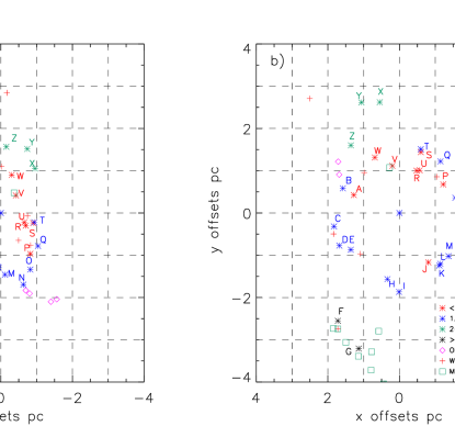
Figure 1: a) is the sky view of CND HCN(1-0) clumps (A to Z), water, methanol and OH masers positions relative to the origin SgrA^∗. X and Y axes oriented in direction of increasing RA and Dec (J2000).
b) is the deprojected view of HCN(1-0) clumps and masers and lie in the disk’s plane. Masers are only plotted where the deprojected distances from SgrA^∗ are less than 4pc and their observed los velocities are compatible with CND los velocities.

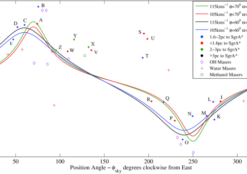
Figure 2: Plots of predicted line of sight velocities generated by varying the PA of the disk’s major axis , $\phi$, and its inclination $\alpha$. As listed in the figure’s legend, rotational velocities of 105 and 115 km s^-1 were adopted as the upper and lower limits bracketing 110 km s^-1 (see Table 7) . Increasing PA shifts the curve horizontally to the left. Increasing the tilt angle increases the peak value of the los velocity. The observed los velocities of HCN(1-0)clumps (A to Z) by (Christopher et al., 2005), water, methanol and OH masers are also plotted.

3 Selection of HCN Clumps for Analysis

LVG analysis is complicated by the lack of data for multi transitions of a trace molecule from a single source. Data for sources that is available has different spatial resolutions since it has been observed with different telescopes at different wavelengths. The analysis relies on modelling emission from three transition levels to produce reliable HCN column densities, hydrogen densities and opacities for the clumps. A literature review led to a choice of two groups of clumps that had been observed in multiple transitions of HCN and that were physically and kinematically related.

The first group of five clumps were collated and labelled A to E by Marr et al. (1993) who observed clumps in H¹³CN 1-0 and HCO⁺ 1-0 and H¹²CN 1-0 (Guesten et al., 1987) channel maps were convolved with a 12$\times$12 Gaussian beam before extracting spectra to allow direct comparison with HCN 3-2 (Jackson et al., 1993) spectra. All the data was produced from unresolved images but had a consistent set of related intensities, spatial and kinematic properties which were modelled by Marr et al. (1993). Our modelling is in effect a re-evaluation of the earlier analysis.

Marr et al. (1993) indicate the rms uncertainties for H¹²CN, H¹³CN and HCO⁺ brightness temperatures are 0.2K which represents an uncertainty for peak brightness temperatures ranging from 4 to 20%. The peak brightness temperatures for HCN 3-2 sourced from Jackson et al. (1993) have a 30% uncertainty.

The dilution factors for clumps A to E were calculated using their corresponding Christopher et al. (2005) clump sizes divided by the 12$\times$12 beam of the telescope used for the HCN 3-2 Jackson et al. (1993) observations. Clump D is not apparent in the 3-2 observations so the average Christopher et al. (2005) clump size of 0.25pc was used to calculate its dilution factor. The dilution factors for the clumps were used to convert the observed peak brightness temperatures in Table 1 of Marr et al. (1993) to resolved temperatures in Table 1.

Table 1: Properties of 1st Clump Group

Clump		Tracer	Resolved	Central	Line Width	Dilution	Maximum Brightness
Labels	Labels		Diameter	Velocity	dV	Factor	Temperature Tb
							Observed	Resolved
			pc	kms-1	kms-1		K	K
A	D	H12CN	0.17	102	50	0.093	3.6	39
		HCO+					3.4	37
		H13CN					0.8	9
		HCN 3-2					4.4	47
B	W	H12CN	0.27	65	60	0.234	4.8	21
		HCO+					3.4	14.5
		H13CN					1.3	5.6
C	Z	H12CN	0.24	55	60	0.185	2.9	16
		HCO+					3.0	16
		H13CN					1.3	7
		HCN 3-2					2.5	13.5
D	na	H12CN	0.25	85	75	0.200	3.0	15
		HCO+					$\leq$1.0	5
		H13CN					0.7	3.5
		HCN 3-2					2.1	10.5
E	O	H12CN	0.33	-96	88	0.349	4.4	12.6
		HCO+					2.2	6.3
		H13CN					0.7	2.0
		HCN 3-2					5.0	14.3

We selected the second group of seven clumps, labelled D, I, M, O, P, W and Z by Christopher et al. (2005) by comparing locations and their central velocities listed in three separate papers that described observations in three HCN transitions and the HCO⁺(1-0) transition (Christopher et al., 2005; Montero-Castaño et al., 2009; Jackson et al., 1993).

The velocity integrated HCN and HCO⁺ fluxes from Christopher et al. (2005) have an estimated uncertainty of 10%, HCN 4-3 integrated intensities from (Montero-Castaño et al., 2009) have an estimated uncertainty of 0.4K based on the 0.5Jy cut off for the integrated map, equating to about 10% for the peak brightness temperatures. The HCN 3-2 data is the same as used for the first group of clumps. For each transition we estimate a further 5% uncertainty is due to the extraction of peak brightness temperatures from the published spectra.

Four of the seven objects, i.e. clumps D, M, W and Z, have the strongest velocity space correlation and are undoubtedly clumps observed in multiple HCN transitions. Clumps I and O have anomalous central velocities in the 3-2 transition. These observations have been included on the basis that the spectra are unresolved, which can leave greater room for discrepancies and were based on visual inspection of the Jackson et al. (1993) figures. Clump P has a lower central velocity in the HCN(4-3) transition, but has been included on the basis that it was one of the clumps matched by Montero-Castaño et al. (2009) with the HCN(1-0) observations by Christopher et al. (2005). Fig. 7 in Montero-Castaño et al. (2009) shows the (1-0) and (4-3) spectra with double peaks and absorption occurs between the peaks in the (1-0) spectrum which can explain the discrepancies (see Table 2). The larger peak intensity value was used where twin peaks occurred together with the published FWHM spectral widths. All clumps were selected to provide a representative sample through the ring.

It should be noted that central velocities were only quantified by Christopher et al. (2005) in Table 2 of their paper for the (1-0) transition. Central velocities for the (3-2) and (4-3) transitions were estimated from the spectra in the relevant papers. Line widths were listed for the (1-0) and (4-3) transitions but had to be estimated for the (3-2) transition. The (3-2) transition spectral widths are large, due in some measure to the larger telescope beam size (12${}^{{}^{\prime\prime}}$).

Table 2: Properties of 2nd Clump Group

HCN clump		Central Velocity			FWHM			Position rel to SgrA∗
		km s-1			km s-1			$\Delta$X	$\Delta$Y
(1-0)	(4-3)	(1-0)	(3-2)	(4-3)	(1-0)	(3-2)d	(4-3)	pc	pc
D	A	101	100	110	45.5	80.0	38.5	1.09	1.32
I	AA	-18	-50	-25	15.0	80.0	49.5	0.83	-0.38
M	U	-64	-50	-50	19.0	75.0	47.0	-0.21	-1.49
O	Q	-108	-70	-90	36.5	90.0	51.0	-0.81	-1.41
P	N	-73	-75	-40	28.2	75.0	97.0	-0.81	-0.86
W	F	56	45	50	27.9	45.0	40.0	-0.33	0.88
Z	E	58	50	40	39.6	50.0	55.0	-0.10	1.54

Table 2 and Fig. 3 show nine clumps with the observations in three HCN transitions located in reasonable proximity of one another together with the offsets from SgrA^∗ in parsecs for the transition observations. Seven of these nine clumps (D, I, M, O, P, W and Z) have their different transition observations within 7 arcseconds and generally within 2.6 arcsecs of their mean location and the emission can be regarded as arising from the same clump especially given that the uncertainty of the positions of the HCN(3-2) clumps are $\pm 0.25$pc or 6.5 arcsecs due to the telescope’s beam size. Clumps H and L have the (1-0) and (4-3) transitions in close proximity but the (3-2) transition is too distant to be from the same clump. For convenience the clumps chosen for analysis are referred to by the labels given in Christopher et al. (2005).

Four clumps (A, B, C and E) from the first group are in common with clumps (D, W, Z and O) of the second group, allowing a comparison between the results. Our results and conclusions are based on observations of the second group of clumps which are largely resolved.

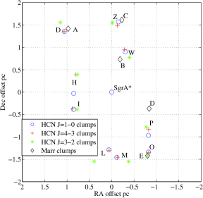
Figure 3: The figure shows positions of the two HCN clump groups selected for LVG modelling. Locations of the first group are marked with black diamonds and have black labels used for Marr et al. (1993) clumps. The location of the second clump group transitions are marked with their respective symbols as shown in the legend and have blue labels used for Christopher et al. (2005) clumps. Offsets from SgrA^∗ are in parsecs based on the J2000 epoch.

4 LVG Modelling

In this section, we use a Large Velocity Gradient model to simultaneously fit HCN and HCO⁺ peak line intensities in order to infer hydrogen number densities, optical depths and the column densities of HCN and HCO⁺ in the CND clumps. Data for the two HCN clump groups selected from Section 3 are analysed. We adopted an ortho to para hydrogen ratio of 3:1 as well as a [He]/[H] ratio of 0.1.

Molecular data for HCN (Green & Thaddeus, 1974) and HCO⁺ (Flower, 1999) was sourced from the Leiden Atomic and Molecular Database (LAMDA). This data included excitation level information, Einstein A coefficients and collision rates for a range of kinetic temperatures and formed part of the input to the LVG code used to analyse the observations. We do not use the HCN database with hyperfine lines in the 1-0 transition as the high degree of overlap of the hyperfine spectra combined with the large velocity width of the observations produce no significant difference from the data set using the single 1-0 transition.

Electron collisions with HCN were not included in our analysis because the estimated low electron fraction of $\leqslant$ 10^-7, corresponding to a hydrogen molecular density of 10⁶cm^-3, would contribute only a small percentage of the total intensity. Given the high column density of the cloud, the ionisation fraction is not expected to exceed 10^-7 whereas significant effects would require the fraction to be $\sim$10^-5. Figures 8a & b from Sternberg & Dalgarno (1995) support this assumption of low ionisation fraction for galactic centre clouds which have an Av of $\sim$27. The cosmic ray ionisation rate would need to be in excess of $5\times 10^{-13}$ s^-1 H^-1 in order to raise the electron abundance to the point that electron collisions are competitive. This is unlikely but may be achievable in the close vicinity of a supernova shock wave, and the circumnuclear ring may be disturbed by the expansion of the Sgr A East supernova remnant (Yusef-Zadeh et al., 2001; Lee et al., 2008).

We checked our LVG code with the RADEX code which uses the same molecular database for less than a 0.5% difference in results, which shows a strong agreement between the two models, given there are presumably differences in radiation fields and allowances for dust emission.

150 K was chosen as the fiducial value for the gas temperature for modelling as this was midway between 250 K, chosen by Marr et al. (1993) and 50 K, used by Christopher et al. (2005). We look at the effect of varying the kinetic temperature in Sections 5.1 and 5.2.

Christopher et al. (2005) quoted dust temperatures varying from 20 to 80 K and adopted 50 K and an Av extinction of 30 in their calculations. Genzel (1989) quoted dust temperatures between 50 and 90 K. Mezger et al. (1989) indicates that cold dust (20 K) within the CND accounts for $\sim$ 90% of the 1.3mm dust emission Wade et al. (1987) found a uniform extinction of $\sim$ 27 towards the central 0${}^{{}^{\prime}}$.5 of the galactic centre. We adopt a dust temperature of 75K and A_V $=$ 26.9 , which is calculated by extrapolating an observed intensity of 2$\times$10¹¹ Jy at 100 $\mu$m Becklin et al. (1982) to the equivalent intensity at 1.3 mm and calculating its associated optical depth which is converted using data provided by Draine & Lee (1984). We found the model proved insensitive to variation of these parameters because the emission frequencies of the molecular tracers are on the low frequency tail of the dust’s IR emission spectrum.

Intensities for the first group of clumps are expressed as resolved peak brightness temperatures obtained by applying dilution factors, which are based on on the FWHM clump diameters listed in Table 2 of Christopher et al. (2005), to the observed radiation temperatures, T_R = I_νc²/2k $\nu^{2}$, listed in Table 1 of Marr et al. (1993). See Table 1 for details.

Peak brightness temperatures for the second group were derived by applying the Rayleigh Jeans formula to integrated intensities from Christopher et al. (2005) for the 1-0 and Montero-Castaño et al. (2009) for the 4-3 transition. Peak brightness temperatures for the 3-2 transition were estimated from spectra in Jackson et al. (1993) and corrected with a dilution factor of 0.2, based on an average FWHM clump size of $6^{{}^{\prime\prime}}.45$ and a telescope beam size of 12${}^{{}^{\prime\prime}}$ $\times$ 12${}^{{}^{\prime\prime}}$.

Each molecule was modelled by starting with local thermal equilibrium (LTE) conditions by choosing a sufficiently high hydrogen number density (10¹² cm^-3), then for each increasing value (dex 0.1) of HCN column density from 10¹² to 10¹⁸ cm^-2 the hydrogen number density was decreased in steps of (dex 0.1) to 10³ cm^-3. The model intensities were plotted as contours on a log-log plot of HCN column density per unit line width at FWHM as abscissa, Ncol/dV, ( cm^-2/(km s^-1)) and hydrogen number density as ordinate, n(H) (cm^-3) . The hydrogen number density and the HCN 1-0 column density per unit line width were inferred from the average of the intersection points of the brightness contours of the four molecular tracers plotted for each clump. The tracers for Group 1 were H¹²CN, H¹³CN , HCO⁺ and HCN 3-2 while HCN 1-0, HCN 3-2, HCN 4-3 and HCO⁺ 1-0 were used for Group 2.

5 Results

5.1 Group 1 Clumps

Table 3 summarises the results from modelling the Group 1 clumps based on observations of H¹²CN 1-0 by Guesten et al. (1987), H¹³CN 1-0 and HCO⁺ 1-0 byMarr et al. (1993) and HCN 3-2 by Jackson et al. (1993). The hydrogen densities varied from 0.5 to 0.9$\times 10^{6}$ cm^-3 and HCN column per unit line width varied from 0.3 to 1.3$\times 10^{14}$ cm^-2kms^-1. Corresponding densities were also recorded for the intersection of the H¹²CN and H¹³CN intensity contours which produced lower hydrogen densities (0.2 to 0.4$\times 10^{6}$ cm^-3) and higher HCN column per line densities (0.3 to 1.8$\times 10^{14}$ cm^-2kms^-1). Table 4 lists the derived parameters for clump A, at the intersection of the H¹²CN and H¹³CN intensity contours for both 150 and 250K gas temperature. The sensitivity to gas temperature shows excitation temperatures at 250 K increased for H¹²CN (190%),HCO⁺ (30%)and HCN 3-2 (105%) but decreased for H¹³CN (24%), while optical depths decreased for all tracers H¹²CN (80%), H¹³CN (17%), HCO⁺ (31%) and HCN 3-2 (180%).

The effect of varying the [¹²C/¹³C] ratio, Z_C, is shown in Fig. 4 where the brightness contour for H¹³CN shifts to the left with decreasing Z_C values. At Z_C = 7 the H¹³CN brightness temperature contour passes through the average of the intersection points and indicates that this is a more representative Z_C value for conditions in the CND than the range of 11 to 28 adapted by Marr et al. (1993).

Table 4 lists the model parameters for clump A, at the intersection of the H¹²CN and H¹³CN brightness contours. Fig. 4 Panel(a): for a gas temperature of T = 150 K shows this point occurs at a lower hydrogen density, higher HCN column density per line width and larger optical depths than the average values obtained for the average intersection point of the HCN transitions, listed in Table 3. Similar values are evident for a gas temperature of 250 K. At these points the molecular hydrogen number density n(H2) is typically 0.4 to 0.25$\times$ 10⁶cm^-3, which about a half to a fifth of the densities for the average of intersection point values obtained above and the density of 10⁶cm^-3 inferred by Marr et al. (1993).

The optical depths at the average point of intersection of individual trace molecules produced optically thin conditions for the 1-0 transitions of H¹²CN, H¹³CN and HCO⁺ and optically thick conditions for the 3-2 transition of HCN. Further the 1-0 transitions of H¹²CN (-0.3 to -0.9) and HCO⁺ (-0.3 to -1.1) were weakly inverted, the optical depth of the 1-0 transition of H¹³CN (-0.3) for Clump A is also weakly inverted.

Panel (c) of Fig. 4 for Clump A shows contours of H¹²CN opacity calculated using H¹²CN and H¹³CN peak brightness temperatures from Molex substituted into Eqn 3 and produces optical depths ranging from 1.0 to 2.0 for a [C¹²]/[C¹³] ratio Z_C = 11, which is the minimum ratio value considered by Marr et al. (1993). They proposed that a consistent model for CND clumps of $\approx 0.1$pc diameter and [HCN]/[H₂] ratio $\approx 0.8\times 10^{-8}$ required assuming values for HCN 1-0 optical depth of 4, a gas temperature of 250 K and a molecular hydrogen density of $\approx$2.6 $\times$ 10⁶ cm^-3. Eqn 3 For clump A, produces a H¹²CN optical depth of 3.4 (150K)and 3.0 (250K) (see Table 4) compared with their value for optical thickness of 4.

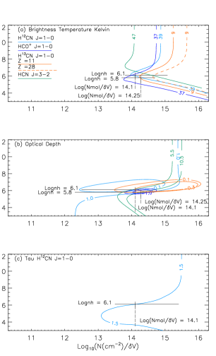
Figure 4: LVG results for Clump A of the first group. The lesser abundant HCO⁺ and H¹³CN, were modelled over a lower range of column densities and plotting consistency with H¹²CN plots maintained by multiplying their column densities per line width by the appropriate abundance ratio to convert them to equivalent H¹²CN column densities which were then divided by their relevant line width.
Panel (a) shows brightness temperature contours for H¹²CN, H¹³CN, HCO⁺ all (1-0) and HCN(3-2). H¹³CN with Z_C = 7 (chain dotted) and Z_C = 28 (dashed) and HCO⁺ with Z${}_{O^{+}}$ = 0.4 (dashed) contours are also plotted. The average intersection point of the species is logn_h = 6.25, log(N_mol/dV) = 14.15 with the intersection of the H¹²/H¹³ contours at log(n_h) = 5.9, logN_Mol/dV) = 14.25. Panel (b) shows optical depth contours for the tracers. One abundance for both H¹³CN and HCO⁺ are plotted as indicated for clarity. H¹²CN, H¹³CN and HCO⁺ are optically thin with inverted transition populations, and HCN(3-2) is optically thick with $\tau$ $\sim$ 1.3. Panel (c) shows the optical depth contours of H¹²CN calculated using brightness temperatures for H¹²CN and H¹³CN from Molex and a [¹²C]/[¹³C] abundance ratio, Z = 11. $\tau^{12}$ $\sim$ 1 at the average intersection point and $\sim$ 2.0 for the closest point of approach of the H¹²CN & H¹³CN brightness contours.

Table 3: Insert Table 3 generated from landscape tables 3 4.tex

Table 4: Insert Table 4 generated from landscape tables 3 4.tex

5.2 Group 2 Clumps

The results for these seven clumps, labelled D, I, M, N, O, P, W and Z after Christopher et al. (2005), were obtained by averaging the values of intersection points of pairs of species and are summarised in Table 5. The molecular hydrogen densities range from n(H$\small{2}$) 0.8 (clump I) to 1.6 (clump M) $\times 10^{6}$cm^-3 for a gas temperature of 150 K; these are less than a quarter to a half of the values for the optically thin scenario of Christopher et al. (2005) for the HCN(1-0) transition. Modelling clumps D and M with a gas temperature of 50 K produces a density, n(H$\small{2}$), of 4.0$\times 10^{6}$cm^-3 (see Table 5).

Table 5 summarises the results for optical depth for the seven clumps where the HCN(1-0) and HCO⁺(1-0) transitions indicate the presence of stimulated emission with negative excitation temperatures and opacities ranging from $-$0.5 to $-$0.25 for 150 K and about 0 for 50 K. The HCN(3-2) opacities range from 1.1 to 2.0 and for HCN(4-3) from 1.0 to 2.6.

The HCN column and molecular hydrogen number densities were obtained from averaging the values of the intersection points of the HCN(1-0) brightness contour with each of the other contours. For example in Fig. 6 for clump W the intersection of HCN(1-0), HCN(4-3) and HCO⁺(1-0) was the lower point at logN${\mathrm{col}}$/$\delta$V = 13.2 and logn_h = 6.1, with the intersection of HCN(1-0) and (3-2) the upper point at log(N_mol/dV) = 13.4 and logn_H = 6.6. The result is an average Column density/$\delta$V of 2 $\times$ 10¹³ cm^-2 and hydrogen density of 0.9 $\times$ 10⁶ cm^-3. It should be noted that the lower limit curve of 12.6 K for the (3-2) transition provides a tighter intersection envelope and slightly lower values for both HCN column and hydrogen number densities.

6 Analysis

In the first group of five clumps, Marr et al. (1993) used a statistical equilibrium excitation model for HCN with values for gas temperature ranging from 150 to 450 K, a dust temperature of 75 K, optical depths from 1 to 12 and [HCN]/[H₂] ratios between 6$\times$ 10^-9 and 3$\times$10^-6. The [¹²C]/[¹³C] ratio (Z_C) was assumed to vary between 10 and 40 while noting that previous estimates varied from 11 (in SgrB2 (Mangum et al., 1988)) to 28 ( in the galactic centre (Wannier, 1989)).

Fig. 4 Panel (a) shows brightness contours for clump A with alternative abundance ratios Z_C $\equiv$ [H¹²CN]/[H¹³CN] = 7 and 28 and Z_O $\equiv$ [HCO⁺]/[HCN] = 0.4 as dashed contours. The alternative ratios of Z_C = 28 and Z${}_{O^{+}}$ = 0.4 do not provide a consistent intersection with the H¹²CN contour. The contours for Z_C = 7 and Z${}_{O^{+}}$ = 0.4 do intersect the H¹²CN contour but at a lower hydrogen density value than for Z_C = 11 and Z${}_{O^{+}}$ = 0.74 which led to the adoption of Z = 11_C and Z${}_{O^{+}}$ = 0.74 for the other clump plots. It should also be noted that the intersection area for all tracers is not representative of the intersection points of the H¹²CN and H¹³CN brightness contours, which occur at higher column density per line width (NCol$\delta$V) values ranging from 0.3 to 1.8$\times 10^{14}$ cm^-2kms^-1 and lower Hydrogen density values of 0.13 to 0.4$\times$10⁶cm^-3.

The effect of changing the Z_C abundance ratio is shown in Fig. 4 Panel(a) where the relevant brightness contours shift to the left as the ratio decreases. This is especially noticeable for the [C¹²]/[C¹³] = 7 curve where the contour falls within the intersection points of the other three species. Similarly, a reduction in the brightness temperature shifts the contour to the left.

The second group of seven HCN clumps provided a good representative sample of CND conditions as they are spread throughout the ring. Clump D is in the North East, clump I is in the East, clump M is in the South, clumps O & P are in the South West and clumps W & Z are in the North (see Fig. 3).

The accuracy of the HCN(3-2) peak brightness temperatures is stated by Jackson et al. (1993) to be $\pm 30\%$ due to the relatively large beam size of about 12”, compared to the average clump size of 6.5”, this also contributed to the large FWHM line widths for this transition compared to the other transitions of HCN and HCO⁺ for this group of clumps (see column 7 of Table 2). The effect of the uncertainty can be seen in the plot of peak brightness temperatures for clump W in Fig. 6, where the contour for the lower peak brightness temperature of 14.7K more closely approaches the average intersection point for the other transitions than does the average HCN(3-2) peak brightness temperature contour of 21K.

Fig. 5 for clump D panel (a) shows contours for three values of the $[\mathrm{HCO^{+}}]/[\mathrm{HCN}]$ abundance ratios, Z${}_{O^{+}}$ = 0.4, 0.74 and 1.2, these variations in the [HCO⁺]/[HCN] emission and absorption ratios are attributable to greater abundances of HCO⁺ in lower density regions both within the CND and along the line of sight (Christopher et al., 2005). Lowering the abundance ratio reduces the column density per line width value. Again in modelling the second group of HCN clumps, the mean HCO⁺ abundance value of 0.74 was used in all plots, in contrast to the value of 0.4 used by Christopher et al. (2005) for regions in the CND with relatively high HCN emission and low HCO⁺ emission.

The molecular hydrogen number density for the seven HCN clumps varies from 1 to 2 $\times 10^{6}$cm^-3, which is an order of magnitude lower than the value n(H₂) of 10⁷cm^-3 reported by Christopher et al. (2005) for HCN(1-0) optically thick gas with ${\tau}$ = 4. Clumps D and M were also modelled using a gas temperature of 50 K, which produced molecular hydrogen densities for both of 4$\times 10^{6}$ cm^-3, which agreed closely with the Christopher et al. (2005) values for optically thin conditions. The brightness temperature value of the HCN(3-2) transition contours in clumps D and O was varied to account for the different dilution factor when using the clump sizes listed in Table 2 of Christopher et al. (2005) instead of the average 0.25 pc size adopted for calculating the 0.2 dilution factor which was felt appropriate for representing the size of all seven clumps. Fig. 5 shows that the HCN(3-2) brightness contour shifts to the left as the brightness temperature decreases, so that it forms a tighter intersection area with the other HCN transitions, this results in slightly lower molecular hydrogen number and HCN column per line width densities than the densities in Table 5.

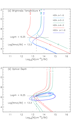
Figure 5: A sample of output for clump D of the second group with gas temperature of 150 K. Panel (a) shows peak brightness temperature contours for HCN (1-0), (3-2), (4-3) and HCO⁺ (1-0). The arithmetic average of the species intersection points is log(n_H) = 6.25, log(NMol/dV) = 13.3. Panel (b) shows the optical depth contours for the HCN(1-0) and HCO⁺(1-0) tracers are optically thin with inverted populations, while the HCN (3-2) and (4-3) transitions are optically thick.

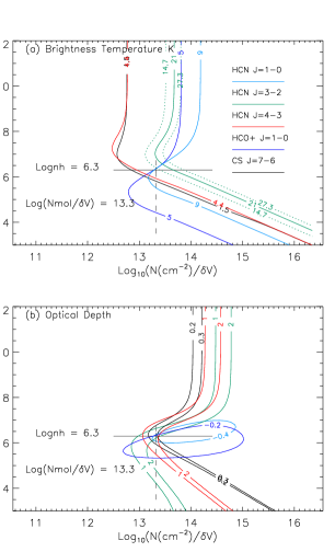
Figure 6: As for Fig. 5 but for clump W. The $\pm 30\%$ uncertainty in (3-2) peak brightness temperatures is shown with the dashed contours in panel(a). CS(7-6) has also been plotted and is consistent for the same physical conditions as HCN(4-3). Panel(b) shows the CS(7-6) is optically thin in contrast with the HCN(4-3) which is optically thick.

Table 5: Insert Table 5 generated by landscape tables 5.tex

7 Discussion

Our LVG modelling shows that molecular hydrogen densities are about 10⁶cm^-3 and optical depths for the HCN(1-0) transition are $\ll$ 1. These results are in marked contrast to the conclusions of Marr et al. (1993) who argue convincingly that an optical depth of 4 in HCN 1-0 leads to higher hydrogen number densities.

Given the errors in flux obtained from the source papers are some 10 to 30% which combined with the systematic errors arising from the calibration of the use of different telescopes ensures that the derived densities could vary by up to a factor of two, so that n(H₂) could range from 0.5 to 1.5 $\times$ 10⁶cm^-3.

As a check on the derived physical conditions the CS(7-6) Montero-Castaño et al. (2009) was modelled for Clump F,which corresponds to Clump W for HCN(1-0). The CS( 7-6) emission defines the same physical conditions as the HCN(4-3) for this clump while the CS(7-6) opacity is thin (0.2) in contrast to an optically thick (2) for HCN(4-3) (see Fig 6).

Marr et al. (1993) argued that if both H¹²CN and H¹³CN occupy the same space, their emissions would have similar beam filling factors and background emissions. Then given equal excitation temperatures for the two species and optical depths that preclude enhanced H¹²CN relative to H¹³CN emission then the ratios of both intensities and opacities would be equal to the ¹²C/¹³C abundance ratio, Z_C.

$$\frac{T_{13}}{T_{12}}=\frac{(1-\mathrm{exp}(-\tau_{13}))}{(1-\mathrm{exp}(-\tau_{12}))}=\frac{\tau_{13}}{\tau_{12}}\quad for\quad\tau_{13}/\tau_{12}\ll 1\\$$ (1)

where the brightness temperature, T =$\lambda^{\!2}$ I_ν/2k, I_ν is the line’s peak intensity and the subscripts 12 and 13 refer to H¹²CN and H¹³CN respectively. In the limit of small opacities for both species Eqn 1 becomes,

$$\frac{T_{12}}{T_{13}}=\frac{[\mathrm{H^{12}CN}]}{[\mathrm{H^{13}CN}]}=Z_{C}\,.$$ (2)

They then argue that the observed H¹³CN emission is optically thin and so the H¹²CN emission is optically thick with the H¹²CN opacity, $\tau$(12), calculated as follows,

$$\large{\tau}\normalsize(12)=-Z\ln\left[1-T(13)/T(12)\right]\,,$$ (3)

This argument hinges on the the assumption that the excitation temperatures of H¹²CN and H¹³CN are similar. However, excitation temperature is very sensitive to the relative populations of the upper and lower states for weakly inverted transitions. The ratio of population levels is given by

$$\frac{n_{2}}{n_{1}}=\frac{g_{2}}{g_{1}}\exp\left(-\frac{h\nu}{\mathrm{kT}_{ex}}\right)\,,\\$$ (4)

then

$$\frac{\mathrm{d}\ln(T_{ex})}{\mathrm{d}\ln(n_{2}/n_{1})} = \frac{kT_{ex}}{h\nu}=\frac{T_{ex}}{4.25\,\mathrm{K}}\,$$ (5)

for the HCN(1-0) transition. When the absolute value of T_ex is large, as it may be for weakly or nearly inverted transitions, small changes in the populations of the upper and lower states can lead to large differences of excitation temperatures.

Table 3 shows excitation temperatures for H¹²CN(1-0) varying between $-$11 and $-$27.6 K for the (1-0) transition and from 5.23 to 19.6 K for H¹³CN. Thus small changes in n₂/n₁ lead to large changes in T_ex. By way of example Fig. 7 shows the H¹²CN and H¹³CN excitation temperatures for (logN_HCN(1-0) = 14.7) depend on hydrogen density. The H¹²CN and H¹³CN excitation temperatures are clearly disparate when the lines are weakly or nearly inverted.

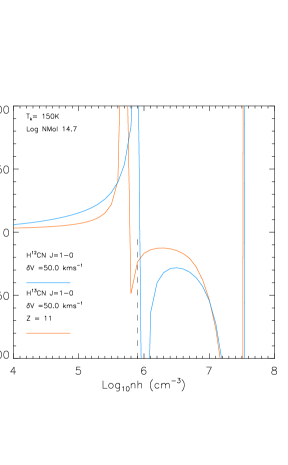
Figure 7: shows the dependence of excitation temperature for the (1-0) transitions of H¹²CN & H¹³CN (1-0) on Hydrogen number density at a column density of 10^14.7. The vertical dashed line at 10^5.9 corresponds to the inferred density for clump A.

Marr et al. (1993) also argued that because HCN and HCO⁺ have similar energy level structures and trace the same gas in the CND the ratio of their abundances is equal to the ratio of their opacities times the ratio of their Einstein A coefficients.

$$\frac{[\mathrm{HCO}^{+}]}{[\mathrm{H^{12}CN}]}=\frac{[\tau\mathrm{HCO}^{+})]}{[\tau\mathrm{H^{12}CN}]}\times\frac{\mathrm{A}_{21}(\mathrm{H^{12}CN})}{\mathrm{A}_{21}(\mathrm{HCO}^{+})}=0.44\times\frac{[\tau\mathrm{HCO}^{+}]}{[\tau\mathrm{H^{12}CN}]}\,.$$ (6)

Using Eqn 6 and the optical depth values from our model for $\tau$ HCO⁺ and $\tau$H¹²CN in Table 4, the [HCO⁺]/[HCN] ratio ranges between 0.4-0.6.

Marr et al. (1993) summarised their results as [HCO⁺]/[H¹²CN] ratio varying between 0.06-0.1, with a [C¹²]/[C¹³] value of Z_C = 30. These [HCO⁺]/[H¹²CN] values were significantly lower than the rates determined from higher resolution observations as between 0.4 and 1.1 (Christopher et al., 2005). Our model used values [HCO⁺]/[H¹²CN] = 0.74 and [H¹²CN]/[H¹³CN] = 11 and produced more consistent intersection points for the peak brightness temperature contour plots of the respective molecules than the abundance values adopted in papers by Marr et al. (1993) and Christopher et al. (2005).

Our modelling produced molecular hydrogen densities from 0.13 and 0.63 $\times 10^{6}$cm^-3 for the first clump group and 1.0 and 2.0 $\times 10^{6}$cm^-3 for the second group at a gas temperature of T = 150 K. Modelling cooler gas, T = 50 K, produced higher densities of 4 $\times 10^{6}$cm^-3, which is consistent with cooler gas being denser but not as dense as proposed by Christopher et al. (2005) who used three scenarios for predicting hydrogen density viz optically thin, virial and optically thick ($\tau$ = 4) without LVG modelling. Our results agree with the optically thin scenario which implies that the clumps are tidally unstable.

Table 6 presents values for the [HCN]/[H₂] ratio based on hydrogen densities and HCN (1-0) column densities per unit line width obtained from our LVG modelling. The HCN densities were calculated by multiplying the HCN column densities per unit line by the appropriate FWHM line width,(dV), and then dividing the resultant HCN column density by the clump size. The [HCN]/[H₂] abundance for the first group was 4.1 $\times 10^{-9}$ and for the second group abundances ranged from 0.2 and 1.2 $\times 10^{-9}$ which is comparable with 10^-9 used by Christopher et al. (2005). Clumps A and E of the first group are the same as clumps D and O of the second group with the higher abundance ratio for the first group resulting from the smaller unresolved clump size 0.1pc compared to the resolved clump sizes of 0.43 and 0.33pc for the second clump group.

Table 6: [HCN]/[H${}_{2}]$ Abundance Ratios from Modelled Clumps

Clump	Kinetic	FWHM	HCN	Line	HCN	HCN	Hydrogen	[HCN]/[H2]
Group	Temp	Diameter	Column Density per	Width	Column	Density	Density	Abundance
ID			line width	dV	Density		n(H2)	Ratio
Pairs	(K)	(pc)	($\times 10^{13}$cm-2/kms-1)	kms-1	($\times 10^{14}$cm-2)	($\times 10^{-4}$cm-3)	($\times$106cm-3)	($\times 10^{-9}$)
First 1
A	150	0.10 2	1.0	50	5.0	16.20	0.397	4.1
E	150	0.10 2	1.0	80	8.0	2.6	0.629	4.1
Second 3
D	150	0.43	2.0	45.5	9.08	6.83	1.26	0.5
D	50	0.43	2.5	45.5	11.40	8.6	3.96	0.2
O	150	0.33	3.2	36.5	8.80	11.3	1.26	0.9
[1] Marr et al. (1993) labels
[2] average clump diameter from Marr et al. (1993)
[3] Christopher et al. (2005) labels

More detailed results can be found in Smith (2012).

8 Conclusions

Our paper selected two groups of clumps observed in multiple transitions of HCN and the(1-0) transition of HCO⁺ that coincided spatially and kinematically. The first group had been selected by Marr et al. (1993) and our analysis is based on our remodelling of their observations. We selected the second group from three separate sources HCN 1-0 and HCO⁺ 1-0 from Christopher et al. (2005), HCN 3-2 from Jackson et al. (1993) and HCN 4-3 from Montero-Castaño et al. (2009).

Data from twenty-six HCN (1-0) clumps listed in Christopher et al. (2005) provided the information for calculating the true (deprojected) clump offsets from SgrA^∗. Eighteen of the twenty-six clumps fit within the accepted range of disk parameters, while seven clumps have velocities that are significantly different from the model disk. The deprojection clearly shows the circular structure of the CND with an inner cavity of radius $\sim$ 1.6 pc. The HCN(1-0) clump line of sight velocities demonstrates the warped nature of the disk’s rotating streams and that the rotational velocity of some streams vary significantly from the accepted 110 km s^-1.

We found that n(H₂) was $\sim$ 10⁶ cm^-3 and $\tau\sim-0.1$ in HCN 1-0 consistent with dust emission and limits based on Genzel et al. (2010). This contradicts the high densities and optical depth $\tau\sim$4 inferred by Christopher et al. (2005) and Montero-Castaño et al. (2009). We show that $\tau\sim$4 is based on the assumption that T_ex for H¹²CN 1-0 and H¹³CN 1-0 is the same and show that this is not the case for the conditions in the CND, where the lines are weakly inverted.

A wider CND survey of the H¹³CN(1-0) transition might clarify the optically thick/thin question and hence the hydrogen density value. An analysis of the NH₃ (1-1), (2-2), (3-3) and (6-6) transitions (Herrnstein & Ho, 2002) would also be useful to check hydrogen densities, particularly as the (6-6) transition traces denser and hotter regions more effectively than HCN. Such a study should be done in the future to reinforce the results of this study.

A possible test of maser effects of negative optical depths in the (1-0) transitions of HCN and HCO⁺ would be to search for a bright (T${}_{b}\sim$ 1000 K) source of continuum emission (such as a quasar or radio galaxy) aligned with one of the disk’s clumps. A comparison of off HCN line frequency, on line frequency of clump observations would then detect an increase of 30 to 60% in the background intensity caused from amplification by HCN(1-0) emission or up to 30% by HCO⁺(1-0) emission as it passes through the clump.

Our results clearly favour the warm, low density scenario with a CND mass of 3 to 4 $\times$ 10⁵ M_⊙ and tidal forces pulling the clumps apart.

Acknowledgements

We thank Maria Montero-Castaño for generously providing the co-ordinates for the HCN(4-3) clumps and Farhad Yusef-Zadeh for providing the co-ordinates of the methanol and water masers detected in the CND.

Appendix A Disk Parameters

A.1 Orientation

The direction of the disk’s major axis is usually specified by its PA East of North, which in this study equates to the complementary angle of $\phi$, and its inclination to the plane of the sky, $\alpha$, as illustrated in Fig. 8. The disk’s axes are designated as x_D with the positive to the left of centre, y_D positive to the top of the figure and z_D positive away form an observer observer’s view along the axis of rotation. Common values of the parameters are given in Table 7.

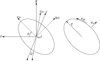
Figure 8: Illustrates the CND’s defining parameters, the left diagram shows the plane of the sky xy with the z axis as the line of sight. x_D, y_D define the disk’s plane with z_D the axis of rotation, $\alpha$ is the angle between z and z_D; $\phi$ is the angle of the disk’s major axis measured clockwise from East in the plane of the sky xy and is the complement of the PA (which is measured East of North). The right hand diagram shows the disk’s physical dimensions: r₀ is the mean radius of the ring; v_ϕ is the rotational velocity; v_r is los velocity, $\Delta$r is radial thickness with FWHM thickness $=r_{0}\sqrt{\mathrm{log4}}=1.18r_{0}$. The thickness perpendicular to the plane of the ring and is assumed to be zero. Typical values for these parameters are listed in Table 7. This figure and Table 7 are based on Fig. 9 and Tables 1 & 2 of Marshall et al. (1995).

Table 7: CND’s Defining Parameters.

	$\alpha$	$\phi$	vϕ	vr	r0	vdisp
	(deg)	(deg)	(km s-1)	(km s-1)	(km s-1)
Previous Estimates1	60-70	60-65	100-110	$<20$	40-50	10-70
Larger Ring2	70		110	52	96	10
HCN3-2 3	59	64	76	-12	38	47
HCN4-3 3	60	65	72	-13	44	40
HCN3-2 4	70$\pm 5$	$\sim 65$	110$\pm 5$	$<19$	39-52
[1] based on Harris et al. (1985); Guesten et al. (1987); Sutton et al. (1990); Jackson et al. (1993)
[2] HI absorption,Liszt et al. (1985)
[3] Marshall et al. (1995)
[4] Jackson et al. (1993)

A.2 Co-ordinate Transformation

Astronomical figures use a 3D axes convention where the x is positive in the easterly direction, the y axis is positive in the northerly direction and the line of sight (z) axis, is positive in the direction away from the observer. The disk co-ordinates have the subscript,D, to distinguish them from the sky co-ordinates.

Rotation matrices can be used to transform plane of sky to plane of disk co-ordinates where co-ordinates in this paper are expressed as offsets from SgrA*. The process is performed in two rotations, the first about the the line of sight (oz) so that the new axes, x${}^{{}^{\prime}}$ and y${}^{{}^{\prime}}$ are at an angle $\phi$ to the xy axes and align with the major and minor axes of the projected disk and the second about the ox${}^{{}^{\prime}}$ axis by an angle $\alpha$ to align a viewer’s line of sight with the disk’s axis of rotation to produce a projection of the disk with true or deprojected dimensions and clump offsets, x_D and y_D from SgrA^∗.

The first transformation is given by

$$\left(\begin{array}[]{c}x^{\prime}\\ y^{\prime}\\ z^{\prime}\end{array}\right)=\left(\begin{array}[]{ccc}\cos\phi&\sin\phi&0\\ -\sin\phi&\cos\phi&0\\ 0&0&1\end{array}\right)\left(\begin{array}[]{c}x\\ y\\ z\end{array}\right)\,.$$ (7)

This second transformation is given by

$$\left(\begin{array}[]{c}x_{D}\\ y_{D}\\ z_{D}\end{array}\right)=\left(\begin{array}[]{ccc}1&0&0\\ 0&\cos\alpha&-\sin\alpha\\ 0&\sin\alpha&\cos\alpha\end{array}\right)\left(\begin{array}[]{c}x^{\prime}\\ y^{\prime}\\ z^{\prime}\end{array}\right)\,.$$ (8)

The transformation from sky to disk co-ordinates is then derived by substituting the matrices from Eqn. 7 into Eqn. 8 to produce

$$\left(\begin{array}[]{c}x_{D}\\ y_{D}\\ z_{D}\end{array}\right)=\left(\begin{array}[]{ccc}\cos\phi\sin\phi&\sin\phi&0\\ -\sin\phi\cos\alpha&\cos\phi\cos\alpha&-\sin\alpha\\ -\sin\phi\sin\alpha&\cos\phi\sin\alpha&\cos\alpha\end{array}\right)\left(\begin{array}[]{c}x\\ y\\ z\end{array}\right)\,.\\$$ (9)

The inverse transformation of Eqn 9 is

$$\left(\begin{array}[]{c}x\\ y\\ z\end{array}\right)=\left(\begin{array}[]{ccc}\cos\phi&-\sin\phi\cos\alpha&-\sin\phi\sin\alpha\\ \sin\phi&\cos\phi\cos\alpha&\cos\phi\sin\alpha\\ 0&-\sin\alpha&\cos\alpha\end{array}\right)\left(\begin{array}[]{c}x_{D}\\ y_{D}\\ z_{D}\end{array}\right)\,,\\$$ (10)

where x_D and y_D, x and y offset are offsets from SgrA^∗ and z_D is the disk’s z co-ordinate which is aligned with its axis of rotation.

A.3 Line of Sight Velocity

A clump’s line of sight velocity along the line of sight velocity is caused by the change in position of the clump in the disk’s plane generating a change in the distance along the line of sight in the sky. The position of a clump in the disk is specified by its x_D and y_D co-ordinates. Evaluation of x_D is straightforward as it is only dependent on the projected x and y co-ordinates. The y_D co-ordinate is dependent on x, y and z co-ordinate values (see Eqn. 10). The projected z co-ordinate along the line of sight is not directly observable, but can be expressed as a function of the projected x and y co-ordinate values and y_D calculated by assuming z_D is zero as there is no independent information available for this quantity and it seems reasonable to adopt this assumption.

The ”line of sight“ velocity from the flat rotation model is then obtained from the following expression:

$$v_{z}=\frac{\mathrm{d}z}{\mathrm{d}t}=\mathrm{v}_{\phi}\cos\phi_{D}\sin\alpha\,.$$ (11)

References

- Becklin et al. (1982) Becklin E. E., Gatley I., Werner M. W., 1982, ApJ, 258, 135
- Christopher et al. (2005) Christopher M. H., Scoville N. Z., Stolovy S. R., Yun M. S., 2005, ApJ, 622, 346
- Draine & Lee (1984) Draine B. T., Lee H. M., 1984, ApJ, 285, 89
- Etxaluze et al. (2011) Etxaluze M., Smith H. A., Tolls V., Stark A. A., Gonzalez-Alfonso E., 2011, ArXiv e-prints 1108.0313
- Flower (1999) Flower D. R., 1999, MNRAS, 305, 651
- Genzel (1989) Genzel R., 1989, in M. Morris ed., The Center of the Galaxy Vol. 136 of IAU Symposium, The Circumnuclear Disk (review). pp 393–405
- Genzel et al. (2010) Genzel R., Eisenhauer F., Gillessen S., 2010, Reviews of Modern Physics, 82, 3121
- Ghez et al. (2005) Ghez A. M., Salim S., Hornstein S. D., Tanner A., Lu J. R., Morris M., Becklin E. E., Duchêne G., 2005, ApJ, 620, 744
- Green & Thaddeus (1974) Green S., Thaddeus P., 1974, ApJ, 191, 653
- Guesten et al. (1987) Guesten R., Genzel R., Wright M. C. H., Jaffe D. T., Stutzki J., Harris A. I., 1987, ApJ, 318, 124
- Harris et al. (1985) Harris A. I., Jaffe D. T., Silber M., Genzel R., 1985, ApJL, 294, L93
- Herrnstein & Ho (2002) Herrnstein R. M., Ho P. T. P., 2002, ApJL, 579, L83
- Jackson et al. (1993) Jackson J. M., Geis N., Genzel R., Harris A. I., Madden S., Poglitsch A., Stacey G. J., Townes C. H., 1993, ApJ, 402, 173
- Karlsson et al. (2003) Karlsson R., Sjouwerman L. O., Sandqvist A., Whiteoak J. B., 2003, A&A, 403, 1011
- Lee et al. (2008) Lee S., Pak S., Choi M., Davis C. J., Geballe T. R., Herrnstein R. M., Ho P. T. P., Minh Y. C., Lee S., 2008, ApJ, 674, 247
- Liszt et al. (1985) Liszt H. S., Burton W. B., van der Hulst J. M., 1985, A&A, 142, 237
- Mangum et al. (1988) Mangum J. G., Rood R. T., Wadiak E. J., Wilson T. L., 1988, ApJ, 334, 182
- Marr et al. (1993) Marr J. M., Wright M. C. H., Backer D. C., 1993, ApJ, 411, 667
- Marshall et al. (1995) Marshall J., Lasenby A. N., Harris A. I., 1995, MNRAS, 277, 594
- Mehringer & Menten (1997) Mehringer D. M., Menten K. M., 1997, ApJ, 474, 346
- Mezger et al. (1996) Mezger P. G., Duschl W. J., Zylka R., 1996, A&ARv, 7, 289
- Mezger et al. (1989) Mezger P. G., Zylka R., Salter C. J., Wink J. E., Chini R., Kreysa E., Tuffs R., 1989, A&A, 209, 337
- Montero-Castaño et al. (2009) Montero-Castaño M., Herrnstein R. M., Ho P. T. P., 2009, ApJ, 695, 1477
- Oka et al. (2011) Oka T., Nagai M., Kamegai K., Tanaka K., 2011, ApJ, 732, 120,1
- Oka et al. (2007) Oka T., Nagai M., Kamegai K., Tanaka K., Kuboi N., 2007, Publications of the ASJ, 59, 15
- Pierce-Price et al. (2000) Pierce-Price D., Richer J. S., Greaves J. S., Holland W. S., Jenness T., Lasenby A. N., White G. J., Matthews H. E., Ward-Thompson D., Dent W. R. F., Zylka R., Mezger P., Hasegawa T., Oka T., Omont A., Gilmore G., 2000, ApJL, 545, L121
- Serabyn et al. (1986) Serabyn E., Guesten R., Walmsley J. E., Wink J. E., Zylka R., 1986, A&A, 169, 85
- Serabyn & Lacy (1985) Serabyn E., Lacy J. H., 1985, ApJ, 293, 445