SMaSH: A Benchmarking Toolkit for Human Genome Variant Calling

Abstract

1 Motivation:

Computational methods are essential to extract actionable information from raw sequencing data, and to thus fulfill the promise of next-generation sequencing technology. Unfortunately, computational tools developed to call variants from human sequencing data disagree on many of their predictions, and current methods to evaluate accuracy and computational performance are ad-hoc and incomplete. Agreement on benchmarking variant calling methods would stimulate development of genomic processing tools and facilitate communication among researchers.

2 Results:

We propose SMaSH, a benchmarking methodology for evaluating human genome variant calling algorithms. We generate synthetic datasets, organize and interpret a wide range of existing benchmarking data for real genomes, and propose a set of accuracy and computational performance metrics for evaluating variant calling methods on this benchmarking data. Moreover, we illustrate the utility of SMaSH to evaluate the performance of some leading single nucleotide polymorphism (SNP), indel, and structural variant calling algorithms.

3 Availability:

We provide free and open access online to the SMaSH toolkit, along with detailed documentation, at smash.cs.berkeley.edu.

4 Contact:

ameet@cs.berkeley.edu, pattrsn@cs.berkeley.edu

5 Introduction

Next-generation sequencing is revolutionizing biological and clinical research. Long hampered by the difficulty and expense of obtaining genomic data, life scientists now face the opposite problem: faster, cheaper technologies are beginning to generate massive amounts of new sequencing data that are overwhelming our technological capacity to conduct genomic analyses (Mardis, 2010). Computational processing will soon become the bottleneck in genome sequencing research, and as a result, computational biologists are actively developing new tools to more efficiently and accurately process human genomes and call variants, e.g., SAMTools (Li et al., 2009), GATK (DePristo et al., 2011), Platypus (Rimmer et al., 2012), BreakDancer (Chen et al., 2009), Pindel (Ye et al., 2009), Dindel (Albers et al., 2011), and so on.

Unfortunately, SNP callers disagree as much as 20% of the time (Lyon et al., 2012) and there is even less consensus in the outputs of structural variant algorithms (Alkan et al., 2011). Moreover, reproducibility, interpretability, and ease of setup and use of existing software are pressing issues currently hindering clinical adoption (Nekrutenko and Taylor, 2012). Indeed, reliable benchmarks are required in order to measure accuracy, computational performance, and software robustness, and thereby improve them.

In an ideal world, benchmarking data to evaluate variant calling algorithms would consist of several fully sequenced, perfectly-known human genomes. However, ideal validation data do not exist in practice. Technical limitations, such as the difficulty in accurately sequencing low-complexity regions, along with budget constraints, such as the cost to generate high-coverage Sanger reads, limit the quality and scope of validation data. Nonetheless, significant resources have already been devoted to generate subsets of benchmarking data that are substantial enough to drive algorithmic innovation. Alas, the existing data are not curated, thus making it extremely difficult to access, interpret, and ultimately use for benchmarking purposes.

Due to the lack of curated ground truth data, current benchmarking efforts with sequenced human genomes are lacking. The majority of benchmarking today relies on either simulated data or a limited set of validation data associated with real-world datasets. Simulated data are valuable but do not tell the full story, as variant calling is often substantially easier using synthetic reads generated via simple generative models. Sampled data, as mentioned above, are not well curated, resulting in benchmarking efforts (such as the Genome in a Bottle Consortium (GBC) (Zook and Salit, 2011) and the Comparison and Analytic Testing resource (GCAT) (Comparison and Testing, 2013)) that rely on a single dataset with a limited quantity of validation data.

Rigorously evaluating predictions against a validation dataset presents several additional challenges. Consensus-based evaluation approaches, employed in various benchmarking efforts, e.g., Consortium (2010); Kedes and Campany (2011); DePristo et al. (2011); Comparison and Testing (2013), may be misleading. Indeed, different methods may in fact make similar errors, a fact which remains hidden without ground truth data. In cases where ‘noisy’ ground truth data are used, e.g., calls based on Sanger-sequencing with some known error rate or using SNP chips with known error rates, accuracy metrics should account for the effect of this noise on predictive accuracy. Additionally, given the inherent ambiguity in the VCF format used to represent variants, evaluation can be quite sensitive to the (potentially inconsistent) representations of predicted and ground truth variants. Moreover, due to the growing need to efficiently process raw sequencing data, computational performance is an increasingly important yet to date largely overlooked factor in benchmarking. There currently exist no benchmarking methodologies that – in a consistent and principled fashion – account for noise in validation data, ambiguity in variant representation, or computational efficiency of variant calling methods.

Without any standard datasets and evaluation methodologies, research groups inevitably perform ad-hoc benchmarking studies, working with different datasets and accuracy metrics, and performing studies on a variety of computational infrastructures. Competition-based exercises, e.g., Kedes and Campany (2011); Earl et al. (2011), are a popular route for benchmarking that aim to address some of these inconsistencies, but they are ephemeral by design and often suffer from the same data and evaluation pitfalls described above.

In short, the lack of consistency in datasets, computational frameworks, and evaluation metrics across the field prevents simple comparisons across methodologies, and in this work we make a first attempt at addressing these issues. We propose SMaSH, a standard methodology for benchmarking variant calling algorithms based on a suite of Synthetic, Mouse, and Sampled Human data. SMaSH leverages a rich set of validation resources, in part bootstrapped from the patchwork of existing data. We provide free and open access to SMaSH, which consists of:

• A set of 5 full-genomes with associated deep coverage short-read datasets (real and synthetic);

• 3 contaminated variants of these datasets that mimic real-world use cases (DePristo, 2013) and test the robustness of variant callers in terms of accuracy and required computational resources;

• Ground truth validation data for each genome along with detailed error profiles;

• Accuracy metrics that account for the uncertainty in validation data;

• Methodology to resolve the ambiguity in variant representations, resulting in stable measurements of accuracy; and

• Performance metrics to measure computational efficiency (and implicitly measure software robustness) that leverage the Amazon Web Services cloud computing environment.

SMaSH is designed to facilitate progress in algorithm development by making it easier for researchers to evaluate their systems against each other.

Ideal	Synthetic	Mouse	Sampled Human

Figure 1: An ‘ideal’ benchmarking dataset satisfies three properties: it contains real reads ($\mathbf{R}$), it includes comprehensive validation of the underlying genome ($\mathbf{C}$), and its underlying genome is human ($\mathbf{H}$). SMaSH contains three types of benchmarking datasets, each of which satisfies two of the three desirable properties of an ideal dataset, so as to cover all three properties.

6 Methods

6.1 Benchmarking Datasets

In this section, we describe the benchmarking datasets contained within SMaSH. A ‘benchmarking dataset’ consists of three components. The first two components are the inputs to the variant calling algorithm to be benchmarked, namely short reads generated from next-generation sequencing technology and a reference genome (used for alignment and variant representation). The third component is the validation data (represented via the standard VCF format) that are used to evaluate the quality of an algorithm’s predictions.

The left panel of Figure 1 illustrates the three desired properties of a benchmarking dataset. Ideally, we would like to evaluate variant calling performance on a human genome (H), have access to comprehensive validation (C) of the underlying sequenced genome, and call variants using real reads (R), that is, reads generated by an actual sequencing machine and not a simulator. To the best of our knowledge, no existing dataset satisfies all three properties. Instead, SMaSH consists of three types of benchmarking datasets that satisfy two of these three properties, as depicted in the three panels on the right of Figure 1. Additionally, for each type of dataset, we also include a contaminated version in which the short reads are contaminated with reads from a separate genome, mimicking the impurities that can be introduced in practice while preparing a sample and/or using a contaminated sequencing machine, and thus testing the robustness of variant callers in this challenging and realistic setting. Table 1 summarizes our validation data, and we next provide details about these datasets.

Table 1: Summary of SMaSH’s validation datasets.

Type	Genome	Validation Error	Sequencer	Length (bp)	Insert Size (bp)	Coverage
Synthetic	Venter	none	simNGS	101	400	30x
	Contam. Venter
Mouse	B6 strain	$0.2\%$ (SNP/Indel), $0.3\%$ (SV)	GAIIx	101	-34	58.6x
	Contam. B6 strain
Human	NA12878	$0.04\%$ (SNP), $1\%$ (SV)	HiSeq2000	101	300	50x
	Contam. NA12878		HiSeq2000	101	300	50x
	NA18507		HiSeq2500	100	300	44x
	NA19240		GAIIx	101	296	49x

6.1.1 Synthetic Datasets

We derive our synthetic datasets from J. Craig Venter’s genome (HuRef). We create a diploid sample genome by applying the HuRef variants provided by Levy et al. (2007) to the hg19 reference genome. We simulate Illumina reads from the sample genome using simNGS (Massingham, 2012) with its default settings. Our second dataset uses the same validation data as the first, along with a version of Venter’s short-read data contaminated by similar short-read data derived from an approximation of James Watson’s genome.

Validation Error Profile:

Any errors in HuRef will be carried through to our synthetic genome, and it is likely that errors in HuRef are sequence-context specific. Nonetheless, since the sample genome and the reads are synthetically generated, the VCF files contain noiseless ground truth data.

6.1.2 Mouse Datasets

The mouse datasets leverage existing mouse genomic data associated with the canonical mouse reference as well as from the Mouse Genomes Project (MGP) (Yalcin et al., 2011). From this data, we create benchmarking datasets with real reads and with comprehensive validation, using the canonical homozygous mouse reference as our sample genome (Church et al., 2009). Our first dataset consists of paired-end reads from the B6 mouse strain (Gnerre et al., 2011), a VCF derived from differences between the mouse reference (based on the B6 mouse strain), and a ‘fake’ reference we created using an alternative mouse strain (the DBA mouse strain). Figure 2 illustrates the process by which we create this dataset, and further details are provided in Supplementary Material B.2. Our second dataset uses the same validation data as the first, along with a version of the B6 short reads contaminated by short reads corresponding to a human genome (NA12878). We use these human reads because, to the best of our knowledge, they are the only publicly available reads generated by the same sequencing methodology as the mouse reads (Gnerre et al., 2011).

Validation Error Profile:

There are two main sources of error in this dataset, namely errors in the mouse reference genome itself and genetic differences between the mouse reference genome and the individual from which short reads were produced. Based on calculations detailed in Supplementary Material B.2, we upper bound the error rates for SNPs and indels at $0.2\%$ and the error rate for SVs at $0.3\%$. Finally, it is worth noting that there are systematic differences between mouse and human genomes. Mouse segmental duplication is more intrachromosomal, and human intrachromosomal duplication is more high-identity (Church et al., 2009). As a result, variant calling performance may vary between the mouse and human datasets.

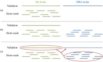
Figure 2: Schematic illustrating process by which SMaSH’s first ‘Mouse’ dataset is generated. (a) Our ideal set up in which the B6 strain (with comprehensive validation and corresponding short reads) serves as the sample and the DBA strain serves as the reference. (b) Publicly available data (note that the B6 validation data are the canonical mouse reference). (c) Construction of an approximate DBA validation set (the ‘fake’ reference) by leveraging a rough set of variants for the DBA strain called relative to the canonical reference.

6.1.3 Sampled Human Datasets

Our real human genomes consist of three well-studied human genomes, including a European female (NA12878), a Nigerian male (NA18507), and a Nigerian female (NA19240). Our validation data consist of subsets of validated SNP and SV information. SMaSH also includes high-coverage Illumina reads for each of these datasets.

We derive our validated SNPs from the intersection of calls from two SNP chips from HapMap2: Perlegen and Illumina BeadArray (Frazer et al., 2007). We chose these chips due to the substantial intersection of their call sites, and because their calls could be readily disambiguated, unlike the two chip technologies used in HapMap3 (HapMap Consortium, 2010). The intersection of their results in NA12878, yields 132K calls, of which 55K are non-reference. Our SV validation data is 169 insertions and deletions called from alignment of finished fosmid sequence (Kidd et al., 2010a, b).

Finally, we include a contaminated version of our NA12878 dataset, in which the NA12878 short reads are contaminated by short reads corresponding to this individual’s husband (NA12877), generated by the same sequencing methodology by Illumina’s Platinum Genomes project.

Validation Error Profile:

The error in our validated SNP data is due to errors in the underlying SNP chip technologies used to generate the data. Moreover, there are various sources of error for our validated SVs, associated with generating and processing the fosmid sequences. As detailed in Supplementary Material B.3, we upper bound the error rate for SNPs at $0.04\%$, and the error rate for SVs at $1.0\%$.

6.2 Evaluation Metrics

We now discuss our set of evaluation metrics of variant calling algorithms against the benchmarking datasets described in Section 6.1. We propose the use of both accuracy and computational performance metrics. Moreover, although SMaSH focuses on reference-based variant calling methods, it does not include alignment-specific metrics, as alignment is an intermediate step (albeit an important one) in the process of variant calling. We believe that improvements in alignment should be measured as a function of their impact on variant calling, both in terms of accuracy and computational performance.

Accuracy: We report two standard metrics from information retrieval. The first metric, recall, measures the ‘probability of calling a validated variant,’ while the second metric, precision, measures the ‘probability that a called variant is correct.’ For SNPs and indels (50bp or less) we measure alternate alleles and exact breakpoints, thus checking zygosity but ignoring phasing. For structural variants, we ignore zygosity, and evaluate left breakpoint and length, both approximately and exactly. In the former case, we use an error tolerance of 100bp, which is within a read-length of the true event and thus sufficiently close to allow for alternative methods, such as targeted assembly, to reconstruct the event. We also present the exact evaluation to highlight variations in accuracy. In some situations, such as our human SNP or SV validation data, the validation data have positive labels but little or no negative labels, and in these situations only recall (and not precision) is reported. Additionally, our computation of recall does not explicitly take into account the impact of sampling in the context of SMaSH’s sampled human benchmarking datasets.

Computational Performance: We use two chief metrics to measure computational performance, namely hours per genome and dollars per genome, and we benchmark performance on Amazon Web Services (AWS). AWS’s cloud infrastructure allows for reproducible benchmarking and ensures robust implementations of variant calling algorithms. When using SMaSH, researchers can benchmark algorithms on AWS using their preferred compute instances, such as single core, multicore, GPU or distributed cluster, and AWS’s pricing mechanism naturally dictates the tradeoff between cost and time. We additionally report more fine-grained performance metrics to help researchers optimize their AWS configuration, including clock time, CPU time, the maximum number of threads used, the maximum disk space required, and the maximum and average amount of memory used during the run of the algorithm.

6.2.1 Accounting for noisy validation data

The performance of an algorithm can only be quantified up to the level of noise in the validation data itself. Since we are working with noisy validation data, it is crucial to capture this uncertainty when reporting results. To do so, we assume that we have an estimate for the number $E$ of validation errors. In settings where we only have positive labels, this estimate captures the number of positive labels that are incorrectly genotyped (either a positive label where there should be none, or a validated variant that is correctly located but incorrectly genotyped). In settings where we have access to both positive and negative labels, this estimate measures either omissions or errors of the type described above.

To quantify these errors, we first note that each called variant can be described via two sets of labels: positive or negative depending solely on the caller, and true or false depending also on the validation dataset. We can compute true positives (TP), false positives (FP) and false negatives (FN) from these two sets of labels. Proposition 1 presents bounds on recall and precision given $E$ and in terms of TP, FP and FN. These bounds hold generally for SNPs, indels and SVs evaluation, and for various evaluation metrics, e.g., metrics considering zygosity, insertion sequence, etc. (see Section D in the Supplementary Material for further details and proof).

Proposition 1.

Let $\mathrm{present}=\mathrm{TP}+\mathrm{FN}$ be the number of positive labels, and let $P=\mathrm{TP}+\mathrm{FP}$ be the number of positive calls. In the case of only positive validated labels,

$$\frac{\mathrm{TP}-E}{\mathrm{present}}\leq\mathrm{recall}\leq\begin{cases}\frac{\mathrm{TP}+E}{\mathrm{present}}&\mbox{if }E\leq\mathrm{FN}\\ \frac{\mathrm{TP}}{\mathrm{present}-E}&\mbox{otherwise.}\end{cases}$$

In the case of both positive and negative labels, the same recall bounds apply, and the following precision bounds hold:

$$\frac{\mathrm{TP}-E}{P}\leq\mathrm{precision}\leq\frac{\mathrm{TP}+E}{P}\,.$$ (1)

Proposition 1 states that recall and precision have worst-case additive errors of the form $E/\mathrm{present}$ and $E/P$, respectively. We use these bounds when reporting results in Section 7.

6.2.2 Ambiguity Resolution

SMaSH incorporates three steps in the evaluation process in order to minimize the impact of VCF ambiguity. The first two steps, cleaning and left normalization, are (standard) VCF preprocessing steps that we perform independently on both the ground truth VCF and the predicted VCF. The cleaning step removes ambiguity associated with case discrepancies, and also filters out extraneous VCF entries, i.e., homozygous reference calls and calls where the reference and alternate allele match. Left normalization involves left shifting all variants as far as possible and is the VCF standard, though this convention is not followed by all variant calling algorithms. Left normalization removes certain types of ambiguity associated with indels and SVs, such as by unambiguously representing the deletion ‘GCGCGC $\rightarrow$ GCGC’ as a deletion event associated with the two leftmost ‘GC’ bases.

Our final step is a novel ambiguity resolution algorithm, Rescue, which involves a second pass over the VCF files during evaluation. After initially strictly comparing the calls between the predicted and the true VCFs, we aim to ‘rescue’ variants marked as incorrect (both false positives and false negatives) due to VCF ambiguity. For each such call, we create two short sequences by expanding the full sequence in some short window around the call in the true and predicted VCF, respectively. We then rescue the call if the two sequences are equivalent. Rescued calls are thus by definition correct, and notably, Rescue can only improve the quality of the reported precision and recall figures. Nonetheless, the number of calls that Rescue is able to rescue is dependent on the window size, as discussed in Section 7.1.

See Section E in the Supplementary Material for further algorithmic details, including discussions about edge cases such as overlapping alleles and combinations of alleles that cancel out.

Table 2: Effect of the window size parameter in the Rescue algorithm on indel precision and recall for mpileup and GATK on the Venter genome. Error bounds are excluded since there is no uncertainty in the Venter validation data.

	mpileup				GATK
	Insertions		Deletions		Insertions		Deletions
Window	Prec	Rec	Prec	Rec	Prec	Rec	Prec	Rec
25	85.8%	70.9%	91.2%	75.2%	90.3%	87.8%	91.9%	90.6%
50	85.8%	70.9%	91.3%	75.2%	90.6%	88.1%	92.3%	90.9%
100	85.8%	70.9%	91.3%	75.2%	90.6%	88.1%	92.3%	90.9%
150	85.7%	70.9%	91.3%	75.2%	90.5%	88.1%	92.2%	90.8%

6.3 Usage

All the materials necessary to run SMaSH are available at our website, smash.cs.berkeley.edu. All relevant files are available for download, including BWA-aligned BAM files containing the raw reads, ground truth VCF files and reference files. All scripts used to calculate results are available in a public repository at github.com/amplab/smash, including evaluation, rescue, VCF normalization and contamination scripts. All data included in SMaSH are derived from publicly available sources and thus can be freely redistributed.

We provide detailed instructions for running SMaSH on AWS. For a researcher wishing to benchmark a new aligner, we describe how to download the short reads, run the aligner on AWS, execute some or all of the variant callers evaluated in Section 7 and run the SMaSH evaluation scripts to get performance and accuracy metrics. In contrast, for a researcher with a new variant caller, we describe how to download our aligned BAM files, run the caller on AWS and evaluate the overall performance and accuracy.

Finally, we plan to update SMaSH as new validated datasets become available. We also invite users to submit performance and accuracy results associated with new aligner and variant caller pipelines to our results page.

Table 3: Effect of ambiguity resolution on benchmarking GATK and mpileup on indels using the mouse dataset. The results illustrate the impact of each successive step of resolution, namely, cleaning, left normalization and rescuing.

	mpileup				GATK
	Insertions		Deletions		Insertions		Deletions
Strategy	Pre	Rec	Pre	Rec	Pre	Rec	Pre	Rec
Cleaning	81.1 $\pm$ 3.5	12.2 $\pm$ 0.5	75.2 $\pm$ 3.3	12.6 $\pm$ 0.6	73.1 $\pm$ 0.4	86.4 $\pm$ 0.5	68.9 $\pm$ 0.4	91.2 $\pm$ 0.6
Normalization	76.6 $\pm$ 0.5	66.5 $\pm$ 0.4	76.6 $\pm$ 0.5	74.9 $\pm$ 0.5	85.7 $\pm$ 0.4	84.0 $\pm$ 0.4	80.5 $\pm$ 0.4	89.9 $\pm$ 0.5
Rescue	87.8 $\pm$ 0.5	76.6 $\pm$ 0.4	79.0 $\pm$ 0.4	85.9 $\pm$ 0.5	92.0 $\pm$ 0.5	86.2 $\pm$ 0.4	85.5 $\pm$ 0.4	91.8 $\pm$ 0.5

Table 4: Benchmarking results for SNPs.

dataset	mpileup				GATK
	Hours	Cost	Pre	Rec	Hours	Cost	Pre	Rec
Venter	$2h$	$\$5$	$98.7\%\pm 0.0$	$97.0\%\pm 0.0$	$57h$	$\$142$	$99.3\%\pm 0.0$	$91.7\%\pm 0.0$
contam. Venter	$3h$	$\$8$	$91.3\%\pm 0.0$	$96.7\%\pm 0.0$	$75h$	$\$188$	$98.7\%\pm 0.0$	$91.8\%\pm 0.0$
NA12878	$5h$	$\$13$	-	$98.8\%\pm 0.0$	$86h$	$\$215$	-	$98.8\%\pm 0.0$
contam. NA12878	$5h$	$\$13$	-	$98.8\%\pm 0.0$	$110h$	$\$275$	-	$98.8\%\pm 0.0$
NA18507	$4h$	$\$10$	-	$99.0\%\pm 0.0$	$154h$	$\$385$	-	$99.0\%\pm 0.0$
NA19240	$4h$	$\$10$	-	$98.7\%\pm 0.0$	$167h$	$\$418$	-	$99.0\%\pm 0.0$
mouse	$6h$	$\$15$	$98.4\%\pm 0.2$	$87.3\%\pm 0.2$	$107h$	$\$268$	$97.8\%\pm 0.2$	$94.9\%\pm 0.2$
contam. mouse	$5h$	$\$13$	$98.3\%\pm 0.2$	$86.7\%\pm 0.2$	$96h$	$\$240$	$97.9\%\pm 0.2$	$94.6\%\pm 0.2$

Table 5: Benchmarking results for small deletions (excluding Pindel results).

dataset	mpileup				GATK
	Hours	Cost	Pre	Rec	Hours	Cost	Pre	Rec
Venter	$2h$	$\$5$	$91.3\%\pm 0.0$	$75.2\%\pm 0.0$	$57h$	$\$142$	$92.3\%\pm 0.0$	$90.9\%\pm 0.0$
contam. Venter	$3h$	$\$8$	$91.7\%\pm 0.0$	$71.7\%\pm 0.0$	$75h$	$\$188$	$92.4\%\pm 0.0$	$90.5\%\pm 0.0$
mouse	$6h$	$\$15$	$79.0\%\pm 0.4$	$85.9\%\pm 0.4$	$107h$	$\$268$	$81.5\%\pm 0.4$	$95.8\%\pm 0.4$
contam. mouse	$5h$	$\$13$	$80.4\%\pm 0.4$	$84.9\%\pm 0.4$	$96h$	$\$240$	$82.8\%\pm 0.4$	$95.6\%\pm 0.4$

Table 6: Benchmarking results for long deletion (approximate evaluation with breakpoint tolerance of 100bp).

dataset	Pindel				BreakDancer
	Hours	Cost	Pre	Rec	Hours	Cost	Pre	Rec
Venter	$80h$	$\$200$	$14.2\%\pm 0.0$	$43.3\%\pm 0.0$	$2h$	$\$5$	$6.9\%\pm 0.0$	$4.9\%\pm 0.0$
contam. Venter	$>400h$	$>\$1000$	-	-	$1h$	$\$2$	$0.0\%\pm 0.0$	$0.0\%\pm 0.0$
NA12878	$81h$	$\$203$	-	$78.3\%\pm 2.9$	$3h$	$\$7$	-	$95.7\%\pm 2.9$
contam. NA12878	$>400h$	$>\$1000$	-	-	$>400h$	$>\$1000$	-	-
NA18507	$168h$	$\$420$	-	$60.0\%\pm 3.0$	$3h$	$\$7$	-	$60.0\%\pm 3.0$
NA19240	$221h$	$\$552$	-	$70.7\%\pm 2.8$	$29h$	$\$73$	-	$77.6\%\pm 2.8$
mouse	$>400h$	$>\$1000$	-	-	$4h$	$\$10$	$18.1\%\pm 1.3$	$11.6\%\pm 0.8$
contam. mouse	$345h$	$\$862$	$6.6\%\pm 4.8$	$53.4\%\pm 0.8$	$3h$	$\$7$	$18.7\%\pm 16.0$	$1.0\%\pm 0.8$

Table 7: Benchmarking results for long deletions (exact evaluation).

dataset	Pindel				Breakdancer
	Hours	Cost	Pre	Rec	Hours	Cost	Pre	Rec
Venter	$80h$	$\$200$	$0.0\%\pm 0.0$	$40.6\%\pm 0.0$	$2h$	$\$5$	$0.0\%\pm 0.0$	$0.2\%\pm 0.0$
contaminated Venter	$>400h$	$>\$1000$	-	-	$1h$	$\$2$	$0.0\%\pm 0.0$	$0.0\%\pm 0.0$
NA12878	$81h$	$\$203$	-	$78.3\%\pm 2.9$	$3h$	$\$7$	-	$0.0\%\pm 2.9$
contaminated NA12878	$>400h$	$>\$1000$	-	-	$>400h$	$>\$1000$	-	-
NA18507	$168h$	$\$420$	-	$60.0\%\pm 3.0$	$3h$	$\$7$	-	$0.0\%\pm 3.0$
NA19240	$221h$	$\$552$	-	$70.7\%\pm 2.8$	$29h$	$\$73$	-	$5.2\%\pm 2.8$
mouse	$>400h$	$>\$1000$	-	-	$4h$	$\$10$	$0.0\%\pm 1.3$	$0.1\%\pm 0.8$
contaminated mouse	$345h$	$\$862$	$0.0\%\pm 4.8$	$52.3\%\pm 0.8$	$3h$	$\$7$	$0.0\%\pm 16.0$	$0.0\%\pm 0.8$

Table 8: Computational performance statistics for the Venter dataset.

caller	Clock Time	Cost	CPU Time	Max Threads	Max disk	Max memory	Avg. memory
mpileup	$2h$	$\$5$	$28h$	$24$	$0.9$ GB	$59.1$ GB	$58.8$ GB
GATK	$57h$	$\$142$	$179h$	$16$	$530$ GB	$59.1$ GB	$53.4$ GB
Pindel	$80h$	$\$200$	$80h$	$1$	$3.4$ GB	$59.1$ GB	$58.7$ GB
BreakDancer	$2h$	$\$5$	$2h$	$1$	$0.02$ GB	$59.1$ GB	$58.7$ GB

7 Results

In this section, we first evaluate the impact of our ambiguity resolution algorithms. We next illustrate the utility of SMaSH by evaluating the performance of some leading SNP, indel, and structural variant calling algorithms. The goal of these experiments is to highlight SMaSH’s functionality, and to simplify the discussion, we use the default settings for all variant calling algorithms and the same machine instance in all of our EC2 experiments. We note that improved accuracy and computational performance results may indeed be possible via parameter tuning and optimizing to minimize EC2 instance footprints.

In all reported results, evaluation is reported as described in Section 6.2. See Section G in the Supplementary Material for further implementation details.

7.1 Ambiguity Resolution

We first examine the precision and recall rates for mpileup and GATK as a function of this user-specified window parameter, as Table 2 illustrates. We see that precision and recall are quite robust to various window sizes. Nonetheless, for small windows ($\leq 25$bp), comparatively fewer true positives are rescued, likely due to the omission of variants associated with an ambiguously represented event. Meanwhile, large windows ($\geq 150$bp) also lead to fewer rescues, likely due to nearby false positives unrelated to the ambiguously represented event entering the window. We observe that a $50-100$bp window balances these two tradeoffs, and we use a $50$bp window in all subsequent experiments for computational reasons.

Next, Table 3 shows the impact of each of the three ambiguity resolution steps. The results show that all three steps significantly impact the precision and recall of both GATK (DePristo et al., 2011) and mpileup (Li et al., 2009) on calling indels for the mouse dataset. Our ambiguity resolution has a similar impact on indel detection for the Venter dataset, and also has a significant (though less drastic) impact on SNP detection for both datasets (see Section E in the Supplementary Material for further results).

7.2 SNP Calling

We benchmark the performance of GATK and mpileup to call SNPs, and Table 4 summarizes the results. The results show that GATK is more computationally expensive, but does not strictly outperform mpileup on the uncontaminated datasets. Moreover, the effect of contamination on precision is fairly visible on Venter, where mpileup’s accuracy clearly degrades while GATK appears robust to the contamination. The difference in performance on the mouse and contaminated mouse dataset is less pronounced, since, as noted in Section F (Supplementary Material), the aligner was able to filter the contaminated reads before they were processed by mpileup or GATK.

7.3 Indel Calling

We evaluate the performance of mpileup, GATK and Pindel on the detection of indels, in particular insertions or deletions 50bp or less, with detailed results presented in Table 5, Table S6, and Table S7. These results demonstrate that GATK and Pindel outperform mpileup in terms of accuracy, but are more expensive computationally. In fact, Pindel highlights the importance of SMaSH’s computational performance metrics, as it failed to complete within our predetermined time limit of 400 hours (i.e., a $\$1000$ AWS budget) on both the contaminated Venter and mouse datasets, and we thus did not obtain results for these experiments. On both contaminated Venter and contaminated mouse, mpileup and GATK gained slightly in precision and worsened in recall as compared to their uncontaminated counterparts. This difference seems to result from the fact that both algorithms predicted fewer indels overall on the contaminated sets than they did SNPs; for example, mpileup called 2.5% fewer indel deletions on mouse and only 0.5% fewer SNPs. Consistent with the SNP results, however, mpileup was less robust to contamination than GATK.

7.4 Structural Variant Calling

We benchmark Pindel and BreakDancerMax on insertions and deletions greater than 50bp in length, reporting approximate breakpoint results in Table 6 and Table S8 (Supplementary Material). We first note that we do not report results for the several experiments that ran longer than our 400 hour budget, namely BreakDancer on contaminated NA12878 and Pindel on mouse, contaminated Venter and contaminated NA12878. On the experiments that did complete, we observe that (perhaps unsurprisingly) SV accuracy is much lower than SNP and indel accuracies, and in particular both Pindel and BreakDancer have fairly low accuracy on long insertions. Indeed, for NA12827, BreakDancer misses all insertions even though it accurately identifies more than half of the deletions. Moreover, we observe that BreakDancer’s recall is much higher for the sampled human datasets than for Venter and mouse. This discrepancy can be explained by the fact that, unlike the sampled NA12878 validation data, the comprehensive Venter and mouse datasets contain many short structural deletions, and BreakDancer is not designed for shorter variants.

We observe drastically different results when evaluating the exact breakpoint of accuracy of these methods (see Table 7 and Table S9). Indeed, both algorithms suffer significant decreases in accuracy under this more stringent evaluation metric. The precision for both algorithms on all applicable datasets approaches zero, and BreakDancer makes almost no exactly accurate calls for insertions or deletions. Pindel, however, does identify some long insertions and deletions by exact breakpoint, thus yielding a minimal degree of recall.

Finally, we note that neither caller handles the contaminated datasets particularly well, though with somewhat different modes of failure. Pindel suffered computationally when dealing with the contaminated datasets, failing to complete on the contaminated Venter and the contaminated NA12878 datasets, and required 375 hours to process the contaminated mouse dataset. Although BreakDancer did not complete on the contaminated NA12878 dataset, it in fact executed very quickly on both the contaminated Venter and contaminated mouse datasets. However, its accuracy suffered greatly relative to its accuracy on the analogous non-contaminated datasets, as it found almost no variants in either case.

7.5 Computational Performance

Although the cost of running a given caller on Amazon’s AWS platform provides a convenient single metric for comparison, we also provide more fine-grained computational performance metrics to highlight differences between the callers and to help researchers optimize their choice of computational platforms. In Table 8 we present the performance metrics for all four callers on the Venter dataset (see Table S10 in Supplementary Material for statistics on other datasets). All four callers use virtually all 60.5GB of memory available to them on Amazon’s cc2.8xlarge instance; mpileup, Pindel, and BreakDancer do so consistently through their runs, but GATK’s memory usage fluctuates as shown by its lower average memory usage, most likely because only portions of the GATK pipeline are multi-threaded. GATK also requires a large amount of disk space, while mpileup and Pindel use only modest amounts; since BreakDancer’s output is in a more compact format than VCF, it requires almost none. We also note that since Pindel became memory-bound on our chosen instance type, we ran it single-threaded; we thus ran BreakDancer on a single thread for consistency.

8 Discussion

Hundreds of variant calling algorithms have been proposed, and the majority of these algorithms have been benchmarked in some form (see detailed discussion in Section A in the Supplementary Material). To the best of our knowledge, none of these existing benchmarking methodologies account for noise in validation data, ambiguity in variant representation, or computational efficiency of variant calling methods in a consistent and principled fashion. Given the rapid growth of next-generation sequencing data, the need for a robust and standardized methodology has never been greater.

The IT industry serves as an illuminating case-study in the context of benchmarking. Similar to next-generation sequencing technology, the IT industry has benefited greatly from the additional hardware resources provided by Moore’s Law. However, the industry’s rapid progress also hinged on the agreement on proper metrics to measure performance as well as consensus regarding the best benchmarks to run to fairly evaluate competing systems (Patterson, 2012). Prior to this industry-wide agreement, each company invented its own metrics and ran its own set of benchmarking evaluations, making the results incomparable and customers suspicious of them. Even worse, engineers at competing companies were unable to determine the usefulness of their competitors’ innovations, and so the competition to improve performance occurred only within companies rather than between them. Once the IT industry agreed on a fair playing field, progress accelerated as engineers could see which ideas worked well (and which did not), and new techniques were developed to build upon promising approaches.

Similarly, we believe that SMaSH could help accelerate progress in the field of genomic variant calling. We have compiled a rich collection of datasets and developed a principled set of evaluation metrics that together allows for quantitative evaluation of variant calling algorithms in terms of accuracy, computational efficiency and robustness/ease-of-use (via ability to run on AWS). Moreover, although SMaSH currently focuses on benchmarking variant calling algorithms for normal human genomes, we believe that the motivating ideas behind SMaSH, along with the tools developed as part of SMaSH, will be useful in devising analogous variant calling benchmarking toolkits for human cancer genomes and for the genomes of other organisms.

Finally, we view SMaSH as a work in progress, as the contents of SMaSH reflect (and are limited by) existing technologies. SMaSH currently has limited ground truth data for human genomes, and the validation data across datasets are enriched in ‘easier’ non-repetitive regions due to underlying sequencing and chip biases. Like any benchmarking suite, SMaSH must evolve over time in order to stay relevant. As new sources of validation data become available, e.g., the NA12878 knowledge base (DePristo and Carneiro, 2013) or curated variants from Illumina platinum genome trios (Illumina, 2013), these datasets should be incorporated into SMaSH. Existing datasets should also be updated to keep them fresh and prevent algorithms from ‘overfitting’ to stale benchmarks, and benchmarking datasets should be deprecated as new data sources obviate their utility.

Appendix A Extended Survey of Related Work

Many variant calling algorithms have been proposed, and the majority of these algorithms have been benchmarked in some form. To the best of our knowledge, none of these existing benchmarking methodologies account for noise in validation data, ambiguity in variant representation, or computational efficiency of variant calling methods in a consistent and principled fashion. Although it is not practical to list all of these past works, in this section we highlight some notable studies that illustrate the current state of benchmarking.

The 1000Genomes Project 1kGenomes10 calls SNPs, indels, and structural variants (SVs) using a rich variety of computational approaches and reports the consensus variant calls of these approaches. The project also invests significant resources to estimate false positive rates by generating an ad-hoc collection of validation data using orthogonal technologies. In contrast to SMaSH, this approach is aimed at validating variants called by specific algorithms, and moreover, the validation efforts of this project vary significantly across algorithm and problem type (e.g., SNPs called from exome sequencing are validated using a different methodology than SVs called from high-coverage full genome sequencing).

The Archon Genomics X PRIZE validation protocol Kedes11 proposes a consensus approach to evaluate variant callers, utilizing a variety of technologies including next-generation sequencing, microarrays, and Sanger sequencing. The developers of the CloudBreak SV caller Whelan13 benchmark their algorithm against a synthetic genome constructed from the Venter genome Levy07, similar to one of SMaSH’s simulated datasets. They also benchmark their calls against the union of SVs called from three earlier studies on a real human, without quantifying the inherent uncertainty in these calls or reconciling differences amongst them. David13 also proposes the simulation of a fake reference, though in the context of parameter selection for their algorithm for Alu detection.

The Genome in a Bottle Consortium (GBC) Zook11 has similar goals as SMaSH, though they have taken a different approach, as they evaluate end-to-end pipelines starting from DNA, target accuracy metrics, and perform evaluations against one specific genome. The Genome Comparison and Analytic Testing resource (GCAT) GCAT in part leverages the validation set from GBC, and performs evaluation of both alignment and variant calling methods using consensus-based and crowdsourced evaluation.

DePristo11 evaluate GATK SNP calling by measuring concordance with HapMap3 Consortium10 and 1000Genomes 1kGenomes10, and by measuring known/new and Ti/Tv ratios. HapMap SNPs Consortium10, Frazer07, Consortium05 are subjected to extensive quality assurance, mainly by measuring consensus across different technologies (SNP chips, PCR sequencing for the ENCODE project, and SNPs from fosmid end sequencing Kidd08), along with a battery of quality control filters largely specific to the technologies involved.

Additional studies have proposed benchmarking techniques for related, yet distinct, problems. The authors of FRCbam Vezzi12 propose methods to assess overall de novo assembly quality and correctness, thus addressing a different problem than the variant calling benchmarking problem that we tackle. The authors of MuTect Cibulskis13, a tool for detecting somatic SNPs in tumor cells, eschew simulated data in favor of benchmarking using downsampling (randomly discarding reads from previous validated datasets to obtain desired coverage) and ’virtual tumors’ (sequencing the same sample twice to test false positive rate, and artificially adding SNPs to real reads to test false negative rate). These techniques are interesting, though they are more applicable to the tumor-normal SNP problem than that of detecting germline mutations (in particular, for germline indels and SVs, downsampling is seldom necessary and artificially altering reads to create SV signatures would be more challenging than doing so for SNPs).

Various studies have also publicly released experimentally validated variant calls for a variety of genomes. These studies provide potentially rich sources of data that could be useful for benchmarking, but the error rates of these variants cannot be easily quantified, and in the case of indels and SVs, most breakpoints are not called to nucleotide resolution. Hence we chose to not incorporate these datasets in the initial version of SMaSH. Just a few examples of such validation data can be found in the following references: SNPs: HapMap3 Consortium10, Mccarroll08; indels: Mills11_insdel; SVs: Mccarroll08, Mills11_CNV, Mills11_insdel; SNPs/indels/SVs: Kidd08, 1000Genomes 1kGenomes10.

Appendix B Data Preparation

B.1 Synthetic Datasets

We derive our synthetic datasets from J. Craig Venter’s genome (HuRef). We did not use the HuRef sequence directly due to the difficulty of computing a most parsimonious VCF “diff” between two full-genome assemblies; optimal alignment algorithms do not scale well enough, and approximate alignment algorithms would not be suitable for benchmarking. Instead, we create the sample genome by applying the HuRef variants provided by Levy07 after ‘lifting over’ Hinrichs06 from hg18 to hg19. This genome features 0.8 million indels and structural insertions and deletions, and 90 inversions. Since all variants in this set come from Levy07, this set lacks much of HuRef’s structural variation Pang10.

We generate reads from the sample genome using simNGS with its default settings. After invoking simNGS, each simulated read is annotated with its associated location in the reference, as well as its location of origin in the sample genome.

To contaminate the Venter reads (Section B.4), we introduced simulate reads from an approximation of James Watson’s genome. We used the variants of dbSNP population 12269, found in Watson, with additional random SNPs sprinkled in, with heterozygous/homozygous ratio 1.2 Levy07 and Ti/Tv ratio 2.1, yielding a 90/10 known/new ratio. We also introduced random structural insertions and deletions of length 1000, yielding 20 megabases of structurally variant sequence Pang10.

B.2 Mouse Datasets

The mouse datasets leverage existing mouse genomic data associated with the canonical mouse reference as well as from the Mouse Genomes Project (MGP). Our first dataset is constructed as follows:

1. Use the canonical homozygous mouse reference as a sample, not as a reference. The canonical mouse reference Church09 (known as ‘mm10’) is derived from the homozygous mouse strain C57BL/6J (abbreviated ‘B6’). In SMaSH, we use mm10 as an extremely well-sequenced sample.

2. Leverage existing short-read data for the B6 strain Gnerre11. Compared with the synthetic and human reads, the mouse reads have a relatively high error rate, as discussed in more detail in Section F, but given their high coverage they are still useful for evaluation of variant calling algorithms. There are ten libraries of paired-end Illumina reads, all from a B6 female. In this paper we consider only the highest-coverage library: 101bp overlapping ends with 58.6x coverage and mean fragment size of 168.

3. Create a reference by applying variation from the Mouse Genomes Project (SNPs, indels, SVs). We leverage a rough set of variants for the DBA mouse strain that are called relative to the mm10 reference. In particular, we use variation from the Mouse Genomes Project consisting of 28K structural variants (SVs), consisting of insertions, deletions, and inversions; 0.9 million indels; and 5.6 million SNPs. After ‘lifting over’ these variants from mm9 to mm10, we create a ‘fake reference’ in which DBA variants are injected into the mm10 reference, and also generate a VCF file storing mm10 variants relative to this ‘fake reference.’

Moreover, our second mouse dataset is a contaminated version of this initial dataset, created from the mouse reads as well as corresponding human reads. The human reads, for NA12878, were generated by the same sequencing methodology Gnerre11, with fragment size mean and standard deviation 155 and 26, versus 168 and 32 for the mouse. See Section B.4 in the Supplementary Material for further details.

Detailed Validation Error Profile:

The first potential source of error is the mm10 assembly itself. On the whole it is “of high fidelity and completeness, and its quality is comparable to, or perhaps better than, that of the reference human genome assembly” Church09. Church09 and Quinlan10 discuss how the mouse reference is imperfect in the $5\%$ of the genome that consists of segmental duplication. However, our validation data (DBA variation extracted from MGP) contain no variants in these highly repetitive regions, and thus only precision (see Section 6.2 for discussion of evaluation metrics) could potentially be affected by these duplications.

Another possible source of error is that the individual from which reads were taken may be slightly genetically different from the individual from which mm10 was constructed, despite both belonging to the inbred strain B6 Watkins08. We provide back-of-the-envelope upper bounds for the number of SNP, indel, and SV differences, by bounding both the number of intervening generations and the mutation rate per generation. To bound the former, note that both mice came from the Jaxson laboratory, whose B6 stock at time of writing Jackson is 235 generations from strain origin. Since the strain is maintained by sibling mating, and the two mice are far more recent than strain origin, then conservatively speaking, there have been fewer than 470 opportunities for generational mutation to strike. The SNP mutation rate is about $10^{-8}$ per generation Egan07. To estimate mutation rates for indels and SVs, we use the approximation of Cartwright09 that for every 100 SNPs, there are at most 16 indels or structural insertions or deletions, whose lengths follow a zeta distribution with parameter roughly $1.7$. Multiplying the resulting mutation rates, the generational gap, and the size of mm10 yields upper bounds of 13k SNPs, 2k indels, and 93 structural insertions and deletions (corresponding to $0.2\%$ error rates for SNPs and indels, and a $0.3\%$ error rate for SVs), affecting the reads in our mouse dataset but not present in the validation data.

B.3 Sampled Human Datasets

Detailed Validation Error Profile:

For our validated SNPs, we have indirect evidence of the error rates of each of the two chip technologies. Perlegen has a 0.51% rate of discrepancy against other HapMap2 calls (Supplementary text 2 of Frazer07). Furthermore, Oliphant02 claim that for SNP chips such as BeadArray, “genotyping should have accuracy above $99\%$”. Therefore, even with a conservative assumption of $2\%$ error rates, and assuming that the errors from the two chips are independent (reasonable since the two chips employ different strategies), our validated SNP data would have error rate $0.04\%$.

Moreover, since the SVs we parsed were called from finished fosmid sequence, understanding the potential sources of error requires understanding the intricate, partially manual process that generated these calls Kidd08, Kidd10insights. A fosmid is a $\sim$40kb fragment of DNA. The Human Genome Structural Variation Project Waterston07 provides libraries of end-sequenced fosmids for 22 individuals. The fosmid ends, each corresponding to a Sanger read, were mapped to the human reference genome. Based on this mapping, each fosmid was classified as concordant or discordant, the latter meaning potentially harboring a SV, for instance due to the ends being close together, far apart, or in opposing orientation. Imprecise SVs were called from clusters of discordant fosmids. Selected discordant fosmids contributing to imprecise SV calls were fully Sanger sequenced, and some of these fully sequenced fosmids were analyzed for SV breakpoints. There are four possible sources of error in the final, precise SV calls:

1. Calling imprecise SVs. Three measures were taken to ensure reliability of these imprecise calls Kidd08. First, discordant fosmids had to pass a series of stringent mapping criteria. Second, fosmids in a cluster had to show the same type of discordancy. Third, putative SV sites were orthogonally validated, e.g., with complete restriction enzyme digests, microarrays, or trio testing.

2. End mapping of a discordant fosmid that is fully sequenced. Given the existence of multiple discordant fosmid ends supporting a particular imprecise SV, an incorrect mapping would require multiple SVs having nearly identical flanking sequences. However, this is unlikely given that the vast majority of SVs have at least 20kb flanking sequences (and the shortest flanking sequence was 8kb). Additionally, an incorrect mapping would likely cause the breakpoint calling step to fail, which Kidd10insights indeed reports to occur, mainly in repetitive regions.

3. Full sequencing of the discordant fosmid. The full sequencing was performed according to the protocols of the Human Genome Project, with error rate pessimistically 1 in 10kb IHGSC2004.

4. Breakpoint calling from the full sequence. Breakpoints were called via human-guided inspection refined by optimal alignment Kidd10insights. The main issue here is alignment ambiguity [Jeff Kidd, personal communication], but this is not a concern to us, as we present SVs in in their full, “ambiguous” form, e.g., TAGCATTAG $\rightarrow$ TAG.

We conclude that despite the complexity of their generation, the SV calls we use are highly reliable. Though we have not performed a full probabilistic analysis, an error rate of $1\%$ seems conservative.

B.4 Contaminated Datasets

One common source of noise in short-read datasets are reads from a separate genome, as might result from impurities introduced in sample preparation or improperly sterilized sequencing machines. In order to benchmark algorithms against this type of data, we created contaminated sets of short reads through a script that walks the target and contaminate set of reads and outputs the contaminate read at a specified likelihood and the target read otherwise. The contaminate reads should have length and insert size as close as possible to the original reads; ideally they should be from the same sequencer, both to simulate real-world contaminated data and to prevent the aligner from filtering out obviously unmatching reads. We chose $10\%$ as the likelihood of contamination for all three of our contaminated datasets. The script used to create these datasets is available to download.

Appendix C Recall and Precision

We now discuss in more detail our motivation for focusing on recall and precision in the context of variant calling validation. Consider the problem of evaluating a variant caller against a ground truth validation set including known variants and known locations lacking variation. In this setting, each called variant is positive or negative (depending solely on the caller) and true or false (depending also on the validation dataset), so we can naively measure performance via four metrics – true positives (TP), false positives (FP), true negatives (TN) and false negatives (FN). However, it would be preferable to use a more succinct set of metrics by distinguishing the behavior of the variant calling algorithm from intrinsic properties of the validation dataset.

To find a convenient parametrization of this four dimensional space, first note that the total numbers of variant presences ($\mathrm{present}=\mathrm{TP}+\mathrm{FN}$) and absences ($\mathrm{absent}=\mathrm{FP}+\mathrm{TN}$) are intrinsic to the dataset, i.e., independent of the caller. Proposition  2 uses these definitions and provides a convenient reparametrization.

Proposition 2.

No information is lost in the coordinate change

$$\{\mathrm{TP},\mathrm{TN},\mathrm{FP},\mathrm{FN}\}\to\{\mathrm{present},\mathrm{absent},\mathrm{recall},\mathrm{precision}\}\,.$$

Proof.

The inverse transformation is readily verified to be

$$\mathrm{TP} =\mathrm{recall}\cdot\mathrm{present}$$

$$\mathrm{FN} =(1-\mathrm{recall})\cdot\mathrm{present}$$

$$\mathrm{FP} =\mathrm{recall}\cdot\mathrm{present}\cdot\left(\frac{1}{\mathrm{precision}}-1\right)$$

$$\mathrm{TN} =\mathrm{absent}-\mathrm{FP}\qed\,.$$

Indeed, $\mathrm{present}$ and $\mathrm{absent}$ are intrinsic to the dataset, that is, independent of the caller, and the space of caller behaviors on a particular dataset can be expressed via the very widespread notions of recall and precision.

Appendix D Noisy Validation Data Bounds

In this section we present details of our analysis of noisy validation data. We wish to derive bounds that will hold regardless of whether we are considering SNPs, indels, or SVs, whether we are considering zygosity, considering insertion sequence in addition to insertion length, etc. To abstract away these details, we assume that there is some set of possible variants, at most one of which is actually present at each site in the reference genome. Then there are three kinds of validation error, at most one of which may occur at a given site: a validated variant where no variant actually exists, a validated variant at the site of a different actual variant, and for a comprehensive dataset, the lack of a validated variant at a site harboring an actual variant.

D.1 Simplified Binary Validation Error Setting

Considering all three types of validation errors presents a fairly complex combinatorial problem. In order to provide intuition for this problem, we first consider the binary case, i.e., we assume that the set of possible variants at each site has size 1. This scenario is not directly applicable to variant calling as it rules out the second kind of validation error described above, but involves fairly straightforward arguments, and provides intuition for subsequent results. We present bounds on recall and precision for this setting in Proposition 3.

Proposition 3.

In the binary setting, the following bounds hold for recall and precision.

Case 1: Positive Validation Only:

$$\frac{\mathrm{TP}-E}{V-E}\leq\mathrm{recall}\leq\frac{\mathrm{TP}}{V-E}\,.$$

Case 2: Positive and Negative Validation:

$$\frac{\mathrm{TP}-E}{P}\leq\mathrm{precision}\leq\frac{\mathrm{TP}+E}{P}$$ (2)

$$\mathrm{recall}\leq\begin{cases}\frac{\mathrm{TP}}{V-E}&\mbox{if }\mathrm{FN}\leq\mathrm{TP}+E\\ \frac{\mathrm{TP}+E}{V+E}&\mbox{otherwise,}\end{cases}$$

$$\mathrm{recall}\geq\begin{cases}\frac{\mathrm{TP}}{V+E}&\mbox{if }\mathrm{FN}\leq\mathrm{TP}-E\\ \frac{\mathrm{TP}-E}{V-E}&\mbox{otherwise.}\end{cases}$$

Note that if $\mathrm{FN}\leq\mathrm{TP}-E$, the recall bounds simplify to

$$\frac{\mathrm{TP}}{V+E}\leq\mathrm{recall}\leq\frac{\mathrm{TP}}{V-E}$$

Proof.

In the case of only positive validated labels, each validation error either goes $\mathrm{TP}\to\mathrm{FP}$ or $\mathrm{FN}\to\mathrm{TN}$, yielding the claimed bounds.

For positive and negative validation data, there are four kinds of validation error: $\mathrm{TP}\leftrightarrow\mathrm{FP}$ and $\mathrm{FN}\leftrightarrow\mathrm{TN}$. The bound on precision is immediate. For recall, first consider finding the upper bound. The two kinds of validation error to consider here are $\mathrm{FP}\to\mathrm{TP}$ and $\mathrm{FN}\to\mathrm{TN}$. Let $a$ be the number of validation errors of the first kind, and $b$ of the second. Then

$$\mathrm{recall}\leq\frac{\mathrm{TP}+a}{\mathrm{TP}+a+\mathrm{FN}-b}$$

Eliminating the extraneous variable $b=E-a$, the derivative of this bound with respect to $a$ vanishes if and only if $\mathrm{FN}=\mathrm{TP}+E$. Therefore, the bound is maximized at either $a=0$ or $a=E$, corresponding to the two cases

$$\mathrm{recall}\leq\begin{cases}\frac{\mathrm{TP}}{V-E}&\mbox{if }\mathrm{FN}\leq\mathrm{TP}+E\\ \frac{\mathrm{TP}+E}{V+E}&\mbox{otherwise.}\end{cases}$$

Computing the lower bound for recall is completely analogous, with $-E$ playing the role of $E$. ∎

D.2 Proof of Proposition 1

Proposition 1 considers the realistic non-binary setting. The resulting bounds look similar to those of Proposition 3, but require more involved analysis as we deal with all three types of validation errors. The complication of the non-binary case is the notion of site. Each site harbors at most one true variant, at most one call, and many true negatives, which we ignore because they are invisible to the metrics of recall and precision. There are five kinds of sites:

• hits $\mathrm{TP}$ where the algorithm calls correctly;

• miscalls $M$, harboring $\mathrm{FP}$ and $\mathrm{FN}$, where there is a true variant but the algorithm calls a different variant;

• wrong silences $S$, harboring $\mathrm{FN}$, where the algorithm fails to make a call when it should;

• false alarms $L$, harboring $\mathrm{FP}$, where the algorithm calls but there is no true variant;

• typical sites $G$, with no call and no true variant.

Note that sites harboring true variants fall under $\mathrm{TP}$, $M$, or $S$; sites lacking true variants fall under $L$ or $G$, and are only relevant in the case of positive and negative validation data.

There are three kinds of validation error:

• A validated variant where no variant actually exists. This can effect $\mathrm{TP}\to L$, transferring $\mathrm{TP}\to\mathrm{FP}$; or $M\to L$ or $S\to G$, decreasing $\mathrm{FN}$.

• A validated variant at the site of a different actual variant. This transfers $\mathrm{TP}\leftrightarrow M$, trading between $\mathrm{TP}$ and the combination of $\mathrm{FP}$ and $\mathrm{FN}$.

• For positive and negative validation data, the lack of a validated variant at a site harboring an actual variant. This is merely the opposite of the first kind of validation error, either transferring $\mathrm{FP}\to\mathrm{TP}$ or increasing $\mathrm{FN}$.

We see immediately that error bounds for precision are the same as the binary case, as the only possible perturbations are $\mathrm{TP}\leftrightarrow\mathrm{FP}$; one direction also increases $\mathrm{FN}$ but this is not relevant to precision.

Next consider the best-case upper bound of recall. There are three ways validation error could increase recall:

• $M\to\mathrm{TP}$;

• $M\to L$ or $S\to G$;

• in the positive and negative validation case, $L\to\mathrm{TP}$.

Letting $a$, $b$, and $c$ be the number of validation errors of those three sorts, respectively, we have

$$\mathrm{recall}\leq\frac{\mathrm{TP}+a+c}{V-b+c}$$

In the best case, $c=0$, so the upper bound will be the same for the positive and negative case as the positive-label case. Since in the best case $a+b=E$, the upper bound is

$$\mathrm{recall}\leq\frac{\mathrm{TP}+a}{V-E+a}$$

with $0\leq a\leq E$. Since the derivative with respect to $a$ vanishes if and only if $E=\mathrm{FN}$, the maximum occurs at $a=E$ or $a=0$, corresponding to the two claimed cases of the upper bound.

Computing the worst-case lower bound of recall is similar, but shakes out a bit differently. There are three ways validation error could decrease recall:

• $\mathrm{TP}\to M$;

• $\mathrm{TP}\to L$;

• in the positive and negative case, $L\to M$ or $G\to S$.

Letting $a$, $b$, and $c$ be the number of validation errors of those three sorts, respectively, we have

$$\frac{\mathrm{TP}-a-b}{V+c-b}\leq\mathrm{recall}$$

In the worst case, $b=0$, and we obtain the desired lower bound in the case of only positive labels, where $c=0$. In the case of positive and negative validation data, in the worst case $a+c=E$, yielding

$$\frac{\mathrm{TP}-a}{V+E-a}\leq\mathrm{recall},$$

which gives us the desired lower bound.

Algorithm 1 SMaSH’s Ambiguity Resolution Algorithm

  Input: Reference ($ref$), True VCF ($vcfTr$), Predicted VCF ($vcfPr$), Rescue window ($win$)

  Output: Recall ($recall$), Precision ($prec$)

  $vcfPr$ = CleanAndLeftNormalize($vcfPr$)

  $vcfTr$ = CleanAndLeftNormalize($vcfTr$)

  $errors$ = Compare($vcfTr$, $vcfPr$)

  $rescued$ = Rescue ($ref$, $vcfTr$, $vcfPr$, $errors$, $win$)

  $errors$ = $errors$ - $rescued$

  $recall$, $prec$ = ComputeResults($vcfTr$, $errors$)

Algorithm 2 Rescue

  Input: Reference ($ref$), True VCF ($vcfTr$), Predicted VCF ($vcfPr$), Validation errors ($errors$), Rescue window ($win$)

  Output: Set of rescued errors ($rescued$)

  $rescued$ = $[\,]$ for $err$ in $errors$

     $strTr$ = ExpandAroundWindow($ref$, $vcfTr$, $err$, $win$)

     $strPr$ = ExpandAroundWindow($ref$, $vcfPr$, $err$, $win$)

     if $strTr==strPr$

        $rescued$.append($error$)

Table S1: Effect of ambiguity resolution on benchmarking GATK and mpileup on SNPs using the mouse dataset. The results illustrate the impact of each successive step of resolution, namely, cleaning, left normalization and rescuing.

	mpileup		GATK
Strategy	Pre	Rec	Pre	Rec
Cleaning	98.4 $\pm$ 0.3	87.2 $\pm$ 0.2	98.1 $\pm$ 0.2	93.5 $\pm$ 0.2
Normalization	98.4 $\pm$ 0.3	87.2 $\pm$ 0.2	98.2 $\pm$ 0.2	93.5 $\pm$ 0.2
Rescue	98.4 $\pm$ 0.3	87.3 $\pm$ 0.2	98.3 $\pm$ 0.2	94.7 $\pm$ 0.2

Table S2: Effect of ambiguity resolution on benchmarking GATK, mpileup and Pindel on SNPs and indels using the Venter dataset. The results illustrate the impact of each successive step of resolution, namely, cleaning, left normalization and rescuing. Error bounds are excluded since there is no uncertainty in the Venter validation data. Top: SNPs, Bottom: Indels.

	mpileup		GATK
Strategy	Pre	Rec	Pre	Rec
Cleaning	96.9	97.0	97.4	91.5
Normalization	96.9	97.0	97.4	91.5
Rescue	98.7	97.0	99.3	91.7

	mpileup				GATK				Pindel
	Insertions		Deletions		Insertions		Deletions		Insertions		Deletions
Strategy	Pre	Rec	Pre	Rec	Pre	Rec	Pre	Rec	Pre	Rec	Pre	Rec
Cleaning	73.2	5.1	78.9	6.5	14.7	13.3	15.8	14.3	10.6	7.5	12.7	9.7
Normalization	84.5	69.7	90.7	74.2	87.5	86.3	89.8	89.2	92.3	71.2	93.8	78.3
Rescue	85.8	70.9	91.3	75.2	90.6	88.1	92.3	90.9	92.7	72.1	94.1	79.2

Appendix E Ambiguity Resolution Details

We now describe the details of the ambiguity resolution algorithm we use when benchmarking variant callers. Input VCF files are first cleaned (removing homozygous reference calls, and calls where the reference and alternate alleles matched) and left-shifted. Next, we perform an initial evaluation in which we loop through the called variants in the predicted and ground truth VCFs. SNPs and short insertions and deletions are strictly compared. Specifically,

• calls where position and alleles match identically are marked as true positives;

• calls in the ground truth VCF but not the predicted VCF, either due to mismatching alleles or no corresponding variant in the predicted VCF, are marked as false negatives; and

• variants in the predicted VCF that have no matching call in the truth VCF are marked as false positives.

Because there are several ways to represent a mutation or set of mutations, we subsequently run the Rescue algorithm in an attempt to match false negatives with false positives within a small window. Algorithm 1 summarizes SMaSH’s ambiguity resolution procedure while Algorithm 2 outlines the steps of the Rescue procedure.

Due to the symmetry of the problem (an allele which is equivalent in the two sets will generate both false positives and false negatives), we need only examine one of these sets. Because it is possible to represent the reference allele itself by a combination of variants which cancel out (for instance an insertion followed by a deletion), we penalize this potential behavior by attempting to rescue only putative false negatives. Tables S1 and S2 provide additional evidence (supporting Table 3 in the main text) of the impact of these three ambiguity resolution steps on variant calling accuracy.

We take the following approach in Rescue for dealing with overlapping alleles within each set (i.e. several overlapping FPs). First, we exclude alleles that have the same starting position; when presented with such a site we select the first of these alleles. Second, for alleles that overlap, all possible combination of variants within the window are checked for equivalence, up to a limit of 16. For instance, consider a 100bp window containing both two overlapping deletions (var1 and var2) and a SNP that overlaps a deletion (var3 and var4). In order to test if these variants result in the same nucleotide sequence as those in the truth VCF, we must construct a reference string from them; but the overlaps render this impossible. Instead, in this example we generate four sequences: those resulting from the pairs (var1,var3), (var2,var3), (var1,var4), and (var2,var4). At a window, each VCF generates a set of sequences in this way, and all pairs of nucleotide sequences are checked for identity. The first pair of sequences which is identical between the two VCFs is marked as a match. The false negatives giving rise to the true sequence become true positives, and the false positives giving rise to the comparison sequence are removed from accounting.

Table S3: Computational performance for BWA alignment.

dataset	BWA
	Hours	Cost
Venter	$60h$	$\$150$
contam. Venter	$23h$	$\$57$
NA12878	$52h$	$\$130$
contam. NA12878	$45h$	$\$112$
NA18507	$37h$	$\$92$
NA19240	$36h$	$\$90$
mouse	$106h$	$\$265$
contam. mouse	$77h$	$\$192$

Appendix F Alignment Statistics

We performed alignment on all benchmarking datasets to evaluate different variant callers in Section 7. All our alignments are performed using BWA 6.1 LiDurbin09 with default settings, except with trimming parameter 15. Table S3 presents the time and cost to run BWA on AWS for each dataset. The resulting BAM files are available at smash.cs.berkeley.edu.

We now provide a summary of the alignment results, starting with Table S4, which presents alignment results for the eight datasets we consider here. We first restrict attention to reads aligning uniquely, yielding the first column of Table S4. The final three columns indicate the percentage of reads that align uniquely with edit distance at most 5, 2, or 0. We also present alternative alignment statistics in Table S5 by restricting attention to reads whose quality scores, after trimming, average 25 and have no more than two “!” values. Note that the mouse (Section 6.1.2) reads have the worst alignment statistics, but the statistics improve dramatically after we perform quality filtering and presumably each variant calling algorithm performs a similar type of filtering before processing the reads.

Note that the percentage of reads aligned for Venter and NA12878 and their corresponding contaminated datasets are almost identical. However, fewer of the contaminated mouse dataset reads were aligned than in the mouse dataset; since the contaminate reads were from a different species, the aligner was evidently better able to filter many of them out.

Table S4: Alignment statistics for BWA.

dataset	aligned	$\leq 5$	$\leq 2$	$=0$
Venter	88.0	99.6	94.5	60.4
contam. Venter	87.8	99.7	94.7	60.8
NA12878	91.3	99.6	97.7	83.8
contam. NA12878	90.9	99.6	97.8	80.9
NA18507	94.4	99.6	96.9	52.3
NA19240	86.2	99.5	95.7	68.8
Mouse	76.2	99.6	93.1	66.8
contam. Mouse	68.4	99.6	93.1	66.7

Table S5: Quality-filtered alignment statistics for BWA.

dataset	aligned	$\leq 5$	$\leq 2$	$=0$
Venter	95.4	99.8	95.5	61.4
contam. Venter	95.4	99.8	95.5	61.4
NA12878	94.8	99.6	97.9	84.5
contam. NA12878	94.7	99.7	98.0	81.5
NA18507	94.4	99.6	97.0	52.9
NA19240	94.0	99.6	96.8	71.9
Mouse	86.8	99.6	93.4	68.6
contam. Mouse	83.2	99.6	93.4	68.5

Appendix G Experimental Details

In this section we describe the details of the experimental setup for the results presented in Section 7.

Computing Platform: All experiments were run on Amazon AWS using cc2.8xlarge instances (8 quad-core processors, 60.5 GB of RAM). Genomics data was stored on EBS and local (ephemeral) storage was configured in RAID0.

SAMtools mpileup: We used SAMtools version 0.1.19-44428cd, which we obtained from the SAMtools sourceforge download page. We followed the ‘basic Command line’ pipeline described on the official mpileup website, using the mpileup option ‘-C50’ as per the recommendation on the mpileup website. We ran mpileup in parallel by chromosome, and concatenated the resulting VCFs using the ‘vcf-concat’ command from VCFtools (note that cc2.8xlarge Amazon instances support up to 32 threads, which is more than the number of chromosomes).

GATK: We ran GATK version 2.6, using the parameters and the pipeline described by the GATK best practices wiki. The pipeline we executed used GATK’s Queue interface to GridEngine, thus ensuring that GATK used as many cores as possible (actual core usage varied at different phases of the analysis due to the ways in which the various steps of the pipeline parallelized).

The final stage in the GATK best practices pipeline is to use known variants as training data to establish the probability of each individual call’s accuracy, so that low-probability calls can be filtered out. For the synthetic and sampled human datasets, we used the hg19 resources from the GATK resource bundle. For the mouse datasets, the dbSNP variants did not overlap enough with our reference to provide a statistically significant prior, so we did not include the variant recalibration step in our GATK mouse pipeline.

Pindel: We ran Pindel version 0.2.4w (May 31 2013) which we obtained from the Pindel repository. We directed Pindel to run on all chromosomes but otherwise used the default parameters. Pindel appears to become memory-bound when working on a high-coverage sample. In particular, on the NA12878 sample, we were unable to run it with multiple threads on the cc2.8xlarge instances (which have only 60.5 GB of memory); however, on a separate machine with 128GB of memory, we were in fact able to run it with multiple threads. Hence, we did not run Pindel in parallel for any of the datasets. Pindel ran for over 400 hours on the contaminated Venter, contaminated NA12878 and mouse datasets; we terminated these jobs before they completed.

BreakDancer: We downloaded breakdancer-max version 1.2.6 (commit 83efb8e) from the BreakDancer software repository, and ran it with its default parameters. In order to be consistent with our experiments with Pindel, we chose not parallelize BreakDancer (though it is indeed possible to do so by scheduling distinct jobs for each chromosome, along with a separate job to identify interchromosomal translocations). BreakDancer’s output provides, for each SV, left and right breakpoints and a length; we use the left breakpoint and length to convert to VCF. BreakDancer ran for over 400 hours on the contaminated NA12878 dataset and was terminated before completion.

Evaluation Script: We first preprocess the input VCF files (predicted and ground truth) via cleaning and left normalization and then compute the counts of true positives, false positives (where applicable), and false negatives using the ambiguity resolution algorithms described in Section 6.2.2 and Section E. Given these counts, we use Proposition 1 to obtain error bounds on recall and precision. Moreover, while evaluating SVs, if an SV has multiple alternate alleles, i.e., multiple possible lengths, we score it as correct if any alternate allele yields the correct length within the error tolerance for length. Within each of the two categories of SVs, insertions and deletions, we score each validated variant against the closest predicted variant.

Known false positives: In our sampled human SNP data, in addition to sites known to be polymorphic in the sample, there are alleles which through validation are known to be false positives, due to sequencing or alignment artifacts rather than underlying genomic variation. Counts of these sites are tabulated to compute estimates of precision for SNP calling (though not unbiased ones).

Appendix H Additional Experiments

We now present additional benchmarking results. Tables S6 and S7 show results on small insertions and deletions, while Tables S8 and S9 provide results for long insertions. It should be noted that the long insertions results are fairly poor across the board; for the mouse and contaminated mouse results, we see very large margins of error because both callers predicted very few long insertions relative to the number of erroneous variants we expect to find in our validated truth data given the upper-bounded rate of error. Moreover, Table S10 presents additional computational performance results to supplement the results in Table 8 in the main text.

plainnat benchmarking_refs

Table S6: Benchmarking results for small deletion (including Pindel results).

dataset	mpileup				GATK				Pindel
	Hours	Cost	Pre	Rec	Hours	Cost	Pre	Rec	Hours	Cost	Pre	Rec
Venter	$2h$	$\$5$	$91.3\%\pm 0.0$	$75.2\%\pm 0.0$	$57h$	$\$142$	$92.3\%\pm 0.0$	$90.9\%\pm 0.0$	$80h$	$\$200$	$94.0\%\pm 0.0$	$79.8\%\pm 0.0$
contam. Venter	$3h$	$\$8$	$91.7\%\pm 0.0$	$71.7\%\pm 0.0$	$75h$	$\$188$	$92.4\%\pm 0.0$	$90.5\%\pm 0.0$	$>400h$	$>\$1000$	-	-
mouse	$6h$	$\$15$	$79.0\%\pm 0.4$	$85.9\%\pm 0.4$	$107h$	$\$268$	$81.5\%\pm 0.4$	$95.8\%\pm 0.4$	$>400h$	$>\$1000$	-	-
contam. mouse	$5h$	$\$13$	$80.4\%\pm 0.4$	$84.9\%\pm 0.4$	$96h$	$\$240$	$82.8\%\pm 0.4$	$95.6\%\pm 0.4$	$345h$	$\$862$	$85.9\%\pm 0.4$	$81.3\%\pm 0.4$

Table S7: Benchmarking results for small insertions.

dataset	mpileup				GATK				Pindel
	Hours	Cost	Pre	Rec	Hours	Cost	Pre	Rec	Hours	Cost	Pre	Rec
Venter	$2h$	$\$5$	$85.8\%\pm 0.0$	$70.9\%\pm 0.0$	$57h$	$\$142$	$90.6\%\pm 0.0$	$88.1\%\pm 0.0$	$80h$	$\$200$	$92.5\%\pm 0.0$	$72.9\%\pm 0.0$
contam. Venter	$3h$	$\$8$	$87.8\%\pm 0.0$	$68.7\%\pm 0.0$	$75h$	$\$188$	$90.9\%\pm 0.0$	$87.5\%\pm 0.0$	$>400h$	$>\$1000$	-	-
mouse	$6h$	$\$15$	$87.8\%\pm 0.4$	$76.6\%\pm 0.4$	$107h$	$\$268$	$91.0\%\pm 0.4$	$91.5\%\pm 0.4$	$>400h$	$>\$1000$	-	-
contam. mouse	$5h$	$\$13$	$88.6\%\pm 0.5$	$75.8\%\pm 0.4$	$96h$	$\$240$	$91.1\%\pm 0.4$	$90.9\%\pm 0.4$	$345h$	$\$862$	$92.4\%\pm 0.5$	$71.7\%\pm 0.4$

Table S8: Benchmarking results for long insertions (approximate evaluation with breakpoint tolerance of 100bp).

dataset	Pindel				BreakDancer
	Hours	Cost	Pre	Rec	Hours	Cost	Pre	Rec
Venter	$80h$	$\$200$	$24.8\%\pm 0.0$	$10.2\%\pm 0.0$	$2h$	$\$5$	$4.2\%\pm 0.0$	$0.0\%\pm 0.0$
contam. Venter	$>400h$	$>\$1000$	-	-	$1h$	$\$2$	$0.0\%\pm 0.0$	$0.0\%\pm 0.0$
NA12878	$81h$	$\$203$	-	$0.0\%\pm 3.0$	$3h$	$\$7$	-	$0.0\%\pm 3.0$
contam. NA12878	$>400h$	$>\$1000$	-	-	$>400h$	$>\$1000$	-	-
NA18507	$168h$	$\$420$	-	$0.0\%\pm 5.0$	$3h$	$\$7$	-	$0.0\%\pm 5.0$
NA19240	$221h$	$\$552$	-	$0.0\%\pm 2.5$	$29h$	$\$73$	-	$0.0\%\pm 2.5$
mouse	$>400h$	$>\$1000$	-	-	$4h$	$\$10$	$1.8\%\pm 35.7$	$0.0\%\pm 0.5$
contam. mouse	$345h$	$\$862$	$8.2\%\pm 82.7$	$1.3\%\pm 0.5$	$3h$	$\$7$	$0.0\%\pm 0.0$	$0.0\%\pm 0.5$

Table S9: Benchmarking results for long insertions (exact evaluation).

dataset	Pindel				Breakdancer
	Hours	Cost	Pre	Rec	Hours	Cost	Pre	Rec
Venter	$80h$	$\$200$	$0.0\%\pm 0.0$	$9.7\%\pm 0.0$	$2h$	$\$5$	$0.0\%\pm 0.0$	$0.0\%\pm 0.0$
contaminated Venter	$>400h$	$>\$1000$	-	-	$1h$	$\$2$	$0.0\%\pm 0.0$	$0.0\%\pm 0.0$
NA12878	$81h$	$\$203$	-	$0.0\%\pm 3.0$	$3h$	$\$7$	-	$0.0\%\pm 3.0$
contaminated NA12878	$>400h$	$>\$1000$	-	-	$>400h$	$>\$1000$	-	-
NA18507	$168h$	$\$420$	-	$0.0\%\pm 5.0$	$3h$	$\$7$	-	$0.0\%\pm 5.0$
NA19240	$221h$	$\$552$	-	$0.0\%\pm 2.5$	$29h$	$\$73$	-	$0.0\%\pm 2.5$
mouse	$>400h$	$>\$1000$	-	-	$4h$	$\$10$	$0.0\%\pm 35.7$	$0.0\%\pm 0.5$
contaminated mouse	$345h$	$\$862$	$0.0\%\pm 82.7$	$1.3\%\pm 0.5$	$3h$	$\$7$	$0.0\%\pm 0.0$	$0.0\%\pm 0.5$

Table S10: Detailed performance statistics for all datasets and algorithms.

dataset	caller	Clock Time	Cost	CPU Time	Max Threads	Max disk	Max memory	Avg. memory
Venter	mpileup	$2h$	$\$5$	$28h$	$24$	$0.9$ GB	$59.1$ GB	$58.8$ GB
Venter	GATK	$57h$	$\$143$	$179h$	$16$	$530$ GB	$59.1$ GB	$53.4$ GB
Venter	Pindel	$80h$	$\$200$	$80h$	$1$	$3.4$ GB	$59.1$ GB	$58.7$ GB
Venter	BreakDancer	$2h$	$\$5$	$2h$	$1$	$0.02$ GB	$59.1$ GB	$58.7$ GB
contam. Venter	mpileup	$3h$	$\$8$	$28$	$24$	$1.1$ GB	$59.1$ GB	$57.5$ GB
contam. Venter	GATK	$75h$	$\$188$	$152h$	$16$	$536$ GB	$59.1$ GB	$52.8$ GB
contam. Venter	Pindel	-	-	-	-	-	-	-
NA12878	mpileup	$5h$	$\$13$	$52h$	$24$	$1.2$ GB	$59.1$ GB	$56.2$ GB
NA12878	GATK	$86h$	$\$215$	$174h$	$16$	$852$ GB	$59.1$ GB	$55.0$ GB
NA12878	Pindel	$81h$	$\$203$	$78h$	$1$	$4.4$ GB	$59.1$ GB	$58.4$ GB
NA12878	BreakDancer	$3h$	$\$7$	$3h$	$1$	$0.05$ GB	$59.1$ GB	$58.6$ GB
contam. NA12878	mpileup	$5h$	$\$13$	$54h$	$24$	$1.6$ GB	$59.1$ GB	$57.1$ GB
contam. NA12878	GATK	$110h$	$\$275$	$242h$	$16$	$878$ GB	$59.1$ GB	$56.6$ GB
contam. NA12878	Pindel	-	-	-	-	-	-	-
contam. NA12878	BreakDancer	-	-	-	-	-	-	-
NA18507	mpileup	$4h$	$\$10$	$43h$	$24$	$1.8$ GB	$59.1$ GB	$57.4$ GB
NA18507	GATK	$154h$	$\$385$	$234h$	$16$	$710$ GB	$59.1$ GB	$41.9$ GB
NA18507	Pindel	$168h$	$\$420$	$167h$	$1$	$4.4$ GB	$59.1$ GB	$58.8$ GB
NA18507	BreakDancer	$3h$	$\$7$	$3h$	$1$	$0.08$ GB	$59.1$ GB	$58.4$ GB
NA19240	mpileup	$4h$	$\$10$	$46h$	$24$	$1.4$ GB	$59.1$ GB	$57.0$ GB
NA19240	GATK	$167h$	$\$418$	$317h$	$16$	$335$ GB	$59.1$ GB	$50.9$ GB
NA19240	BreakDancer	$29h$	$\$73$	$29h$	$1$	$0.09$ GB	$59.1$ GB	$58.9$ GB
mouse	mpileup	$6h$	$\$15$	$71h$	$24$	$1.4$ GB	$59.1$ GB	$59.0$ GB
mouse	GATK	$107h$	$\$268$	$434h$	$16$	$839$ GB	$59.1$ GB	$56.9$ GB
mouse	Pindel	-	-	-	-	-	-	-
mouse	BreakDancer	$4h$	$\$10$	$4h$	$1$	$0.1$ GB	$59.1$ GB	$56.7$ GB
contam. mouse	mpileup	$5h$	$\$13$	$60h$	$24$	$0.7$ GB	$59.1$ GB	$56.2$ GB
contam. mouse	GATK	$96h$	$\$240$	$351h$	$16$	$786$ GB	$59.1$ GB	$56.1$ GB
contam. mouse	BreakDancer	$3h$	$\$7$	$3h$	$1$	$0.08$ GB	$59.1$ GB	$56.5$ GB

References

- Albers et al. [2011] Albers et al. Dindel: Accurate indel calls from short-read data. Genome Research, 21(6):961–973, 2011.
- Alkan et al. [2011] Can Alkan, Bradley P Coe, and Evan E Eichler. Genome structural variation discovery and genotyping. Nature reviews. Genetics, 12(5):363–376, May 2011.
- Chen et al. [2009] K. Chen et al. Breakdancer: an algorithm for high-resolution mapping of genomic structural variation. Nature Methods, 6:677–681, 2009.
- Church et al. [2009] Deanna M Church et al. Lineage-specific biology revealed by a finished genome assembly of the mouse. PLoS biology, 7(5), 2009.
- Comparison and Testing [2013] Genome Comparison and Analytic Testing, 2013. URL http://www.bioplanet.com/gcat.
- Consortium [2010] The 1000 Genomes Project Consortium. A map of human genome variation from population-scale sequencing. Nature, 467(7319):1061–1073, 2010.
- DePristo et al. [2011] M. DePristo et al. A framework for variation discovery and genotyping using next-generation dna sequencing data. Nature Genetics, 43:491–498, 2011.
- DePristo [2013] Mark DePristo. Personal communication, 2013.
- DePristo and Carneiro [2013] Mark DePristo and Mauricio Carneiro. Talk at advances in genome biology and technology, 2013.
- Earl et al. [2011] Dent Earl et al. Assemblathon 1: A competitive assessment of de novo short read assembly methods. Genome Research, 21, 2011.
- Frazer et al. [2007] Kelly A. Frazer et al. A second generation human haplotype map of over 3.1 million SNPs. Nature, 449(7164):851–861, October 2007.
- Gnerre et al. [2011] Sante Gnerre et al. High-quality draft assemblies of mammalian genomes from massively parallel sequence data. PNAS, 108(4):1513–1518, 2011.
- HapMap Consortium [2010] The HapMap Consortium. Integrating common and rare genetic variation in diverse human populations. Nature, 467(7311):52–58, 2010.
- Illumina [2013] Illumina, 2013. URL http://www.illumina.com/platinumgenomes/.
- Kedes and Campany [2011] Larry Kedes and Grant Campany. The new date, new format, new goals and new sponsor of the archon genomics x PRIZE competition. Nature Genetics, 43(11):1055–1058, 2011.
- Kidd et al. [2010a] Jeffrey M. Kidd et al. Characterization of missing human genome sequences and copy-number polymorphic insertions. Nature Methods, 7(5):365–371, 2010a.
- Kidd et al. [2010b] Jeffrey M. Kidd et al. A human genome structural variation sequencing resource reveals insights into mutational mechanisms. Cell, 143(5):837–847, November 2010b. 10.1016/j.cell.2010.10.027.
- Levy et al. [2007] Samuel Levy et al. The diploid genome sequence of an individual human. PLoS Biol, 5(10):e254, September 2007.
- Li et al. [2009] H. Li et al. The sequence alignment/map (sam) format and samtools. Bioinformatics, 25:2078–2079, 2009.
- Lyon et al. [2012] G. Lyon et al. Low concordance of variant calling algorithms in exome sequencing. In 62nd Annual Meeting of The American Society of Human Genetics, 2012.
- Mardis [2010] Elaine R. Mardis. The $1,000 genome, the $100,000 analysis? Genome Medicine, 2:84, 2010.
- Massingham [2012] Tim Massingham. simNGS and simLibrary, 2012. URL http://www.ebi.ac.uk/goldman-srv/simNGS.
- Nekrutenko and Taylor [2012] Anton Nekrutenko and James Taylor. Next-generation sequencing data interpretation: enhancing reproducibility and accessibility. Nature Reviews Genetics, 13:667–672, 2012.
- Patterson [2012] David Patterson. For better or worse, benchmarks shape a field: technical perspective. Communications of the ACM, 55(7), 2012.
- Rimmer et al. [2012] A Rimmer, I. Mathieson, G. Lunter, and G. McVean. Platypus: An integrated variant caller, 2012. URL www.well.ox.ac.uk/platypus.
- Yalcin et al. [2011] Binnaz Yalcin et al. Sequence-based characterization of structural variation in the mouse genome. Nature, 477(7364):326–329, 2011.
- Ye et al. [2009] Kai Ye et al. Pindel: a pattern growth approach to detect break points of large deletions and medium sized insertions from paired-end short reads. Bioinformatics, 25(21):2865–2871, 2009.
- Zook and Salit [2011] Justin M. Zook and Marc Salit. Genomes in a bottle: creating standard reference materials for genomic variation - why, what and how? Genome Biology, 12:P31, 2011.