Cycling Dynamo in a Young Sun: Grand Minima and Equatorward Propagation

Abstract

We assess the global-scale dynamo action achieved in a simulation of a sun-like star rotating at three times the solar rate. The 3-D MHD Anelastic Spherical Harmonic code, using slope-limited diffusion, is employed to capture convection and dynamo processes in such a young sun. The simulation is carried out in a spherical shell that encompasses 3.8 density scale heights of the solar convection zone. We find that dynamo action with a high degree of time variation occurs, with many periodic polarity reversals every 6.2 years. The magnetic energy also rises and falls with a regular period, with two magnetic energy cycles required to complete a polarity cycle. These magnetic energy cycles arise from a Lorentz-force feedback on the differential rotation, whereas the polarity reversals are present due to the spatial separation of the equatorial and polar dynamos. Moreover, an equatorial migration of toroidal field is found, which is linked to the changing differential rotation and to a near-surface shear layer. This simulation also enters a grand minimum lasting roughly 20 years, after which the dynamo recovers its regular polarity cycles.

1. Introduction

The Sun exhibits many time scales from the ten minute lifetimes of granules to multi-millennial magnetic activity modulations. One of the most prominent of these scales is the 11-year sunspot cycle, during which the number of magnetically active regions waxes and wanes. The Sun also possesses longer-term variability of its magnetic activity such as the 88-year Gleissberg cycle (Gleissberg, 1939) and less frequent phenomenon commonly described as grand extrema (Usoskin, 2013). Other main-sequence stars also exhibit cyclical magnetic phenomenon in Ca II, photometric, spectropolarimetric, and X-ray observations (e.g., Baliunas et al., 1996; Hempelmann et al., 1996; Favata et al., 2008; Metcalfe et al., 2010; Fares et al., 2013; Mathur et al., 2013). These observations include solar-mass stars younger than the Sun that also possess magnetic activity cycles, yet they rotate more rapidly than the Sun as a consequence of the low rate of angular momentum loss in such stars (Barnes, 2007). Furthermore, there are hints from both observations and from theory that a star’s magnetic cycle period is closely linked to its rotation rate (e.g., Saar, 2009; Jouve et al., 2010; Morgenthaler et al., 2011). This may imply that the dynamo regime achieved in our simulation of a young sun, which rotates three times faster than the Sun and has a nearly constant magnetic polarity cycle of 6.2 years, can scale up to the solar rotation rate with a polarity cycle period closer to the 22 year cycle of the Sun.

In addition to its large range of time scales, observations of the magnetic field at the solar surface reveal complex, hierarchical structures existing on a vast range of spatial scales. Despite these chaotic complexities, large-scale organized spatial patterns such as Maunder’s butterfly diagram, Joy’s law, and Hale’s polarity laws suggest the existence of a structured large-scale magnetic field within the solar convection zone. On the Sun’s surface active regions initially emerge at mid-latitudes and appear at increasingly lower latitudes as the cycle progresses, thus exhibiting equatorward migration. As the low-latitude field propagates toward the equator, the diffuse field that is comprised of small-scale bipolar regions migrates toward the pole, with the global-scale reversal of the polar magnetic field occurring near solar maximum (e.g., Hathaway, 2010; Stenflo & Kosovichev, 2012).

Consequently, the large-scale field must vary with the solar cycle, likely being sustained through dynamo action deep in the solar interior. It has been suspected for at least 60 years that the crucial ingredients for the solar dynamo are the shear of the differential rotation and the helical nature of the small-scale convective flows present in the solar convection zone (e.g., Parker, 1955; Steenbeck & Krause, 1969; Parker, 1977). Yet even with the advancement to fully nonlinear global-scale 3-D MHD simulations (e.g., Gilman, 1983; Glatzmaier, 1985; Brun et al., 2004; Browning et al., 2006), achieving dynamo action that exhibits the basic properties of Sun’s magnetism has been quite challenging. Nonetheless, recent global-scale simulations of convective dynamos have begun to make substantial contact with some of the properties of the solar dynamo through a wide variety of numerical methods (e.g., Brown et al., 2011; Racine et al., 2011; Käpylä et al., 2012; Nelson et al., 2013a). It is within this vein of modern global-scale modeling that we report on a global-scale 3D MHD convective dynamo simulation utilizing the ASH code that possesses some features akin to those observed during solar cycles.

Nature of the toroidal magnetic field $B_{\phi}$. (a) Snapshot of the horizontal structure of $B_{\phi}$ at $0.95\,\mathrm{R}\,\!\scriptscriptstyle\sun\!$ shown in Mollweide projection, at the time corresponding to the vertical dashed line in (c). This illustrates the azimuthal connectivity of the magnetic wreaths, with the polarity of the field such that red (blue) tones indicate positive (negative) toroidal field. (b) Azimuthally-averaged $\langle B_{\phi}\rangle$ also time-averaged over a single energy cycle, depicting the structure of the toroidal field in the meridional plane. (c) Time-latitude diagram of $\langle B_{\phi}\rangle$ at $0.95\,\mathrm{R}\,\!\scriptscriptstyle\sun\!$ in cylindrical projection, exhibiting the equatorward migration of the wreaths from the tangent cylinder and the poleward propagation of the higher latitude field. The color is as in (a). (d) A rendering of magnetic field lines in the domain colored by the magnitude and sign of $B_{\phi}$, with strong positively oriented field in red, and the strong oppositely directed field in blue.

2. Methods

The 3D simulation of convective dynamo action presented here uses the ASH code to evolve the anelastic MHD equations for a conductive calorically perfect plasma in a rotating spherical shell. ASH solves the necessary equations with a spherical harmonic decomposition of the entropy, magnetic field, pressure, and mass flux in the horizontal directions (Clune et al., 1999; Miesch et al., 2000). A fourth-order non-uniform finite difference in the radial direction resolves the radial derivatives (Featherstone et al., 2013). The solenoidality of the mass flux and magnetic vector fields is maintained through the use of a stream function formalism (Brun et al., 2004). The boundary conditions used are impenetrable on radial boundaries, with a constant entropy gradient there as well. The magnetic boundary conditions are perfectly conducting at the lower boundary and extrapolated as a potential field at the upper boundary.

The authors have implemented a slope-limited diffusion (SLD) mechanism into the reformulated ASH code, which is similar to the schemes presented in Rempel et al. (2009) and Fan et al. (2013). SLD acts locally to achieve a monotonic solution by limiting the slope in each coordinate direction of a piecewise linear reconstruction of the unfiltered solution. The scheme minimizes the steepest gradient, while the rate of diffusion is regulated by the local velocity. It is further reduced through a function $\phi$ that depends on the eigth power of the ratio of the cell-edge difference $\delta_{i}q$ and the cell-center difference $\Delta_{i}q$ in a given direction $i$ for the quantity $q$. This limits the action of the diffusion to regions with large differences in the reconstructed solutions at cell-edges. Since SLD is computed in physical space, it incurs the cost of smaller time steps due to the convergence of the grid at the poles. The resulting diffusion fields are projected back into spectral space and added to the solution.

We simulate the solar convection zone, stretching from the base of the convection zone at $0.72\,\mathrm{R}\,\!\scriptscriptstyle\sun\!$ to the upper boundary of our simulation at $0.97\,\mathrm{R}\,\!\scriptscriptstyle\sun\!$. This approximation omits the near-surface region and any regions below the convection zone. The SLD has been restricted to act only on the velocity field in this simulation. This mimics a lower thermal and magnetic Prandtl number ($\mathrm{Pr}$, $\mathrm{Pm}$) than otherwise attainable through an elliptic diffusion operator. The entropy and magnetic fields remain under the influence of an anisotropic eddy diffusion, with both a radially dependent entropy diffusion $\kappa_{S}$ and resistivity $\eta$. These two diffusion coefficients are similar to those of case D3 from (Brown et al., 2010), with $\kappa_{S},\eta\propto\overline{\rho}^{\;-1/2}$, with $\overline{\rho}$ the spherically symmetric density. The stratification in this case has about twice the density contrast across the domain, being 45 rather than 26, and has a resolution of $N_{r}\times N_{\theta}\times N_{\phi}=200\times 256\times 512$.

3. Cyclical Convective Dynamo Action

Global-scale convective dynamo simulations in rotating spherical shells have recently achieved the long-sought goal of cyclical magnetic polarity reversals with a multi-decadal period. Moreover, some of these simulations have illustrated that large-scale dynamo action is possible within the bulk of the convection zone, even in the absence of a tachocline. Global-scale MHD simulations of a more rapidly rotating Sun with the pseudo-spectral Anelastic Spherical Harmonic (ASH) code have produced polarity reversing dynamo action that possesses strong toroidal wreaths of magnetism that propagate poleward as a cycle progresses (Brown et al., 2011). These fields are seated deep within the convection, with the bulk of the magnetic energy near the base of the convection zone. The perfectly conducting lower boundary condition used here and in those simulations requires the field to be horizontal there, which tends to promote the formation of longitudinal structure in the presence of a differential rotation.

A recent simulation with ASH employs a dynamic Smagorinski diffusion scheme, wherefore they achieve a greater level of turbulent complexity. Those simulations show that the large-scale toroidal wreaths persist despite the greater pummeling they endure from the more complex and vigorous convection (Nelson et al., 2013a). Not only do the toroids of field persevere, but portions of them can be so amplified that the combination of upward advection and magnetic buoyancy create loops of magnetic field (Nelson et al., 2013b). This lends credence to the classical picture of a Babcock-Leighton or Parker interface dynamo (Leighton, 1969; Parker, 1993), with semi-buoyant flux structures that rise toward the solar surface, leading to active regions and helicity ejection. There is the caveat that the magnetic fields in the simulation are instead built in the convection zone.

Implicit large-eddy simulations (ILES) have concurrently paved the road toward more orderly long-term cycles in a setting that mimics the solar interior. Indeed, simulations utilizing the Eulerian-Lagrangian (EULAG) code produce regular polarity cycles occurring roughly every 80 years in the presence of a tachocline and with the bulk of the magnetic field existing at higher latitudes (Ghizaru et al., 2010). This simulation showed radial propagation of structures but little latitudinal variation during a cycle. More recent simulations of a Sun-like star rotating at $3\,\Omega\,\!\scriptscriptstyle\sun\!$ also produce low-latitude poleward propagating solutions (Charbonneau, 2013). Such dynamo action is accomplished first through the reduction of the enthalpy transport of the largest scales through a simple sub-grid-scale (SGS) model that diminishes thermal perturbations over a roughly 1.5 year time scale, which serves to moderate the global Rossby number. The ILES formulation of EULAG also maximizes the complexity of the flows and magnetic fields for a given Eulerian grid resolution.

Convective patterns and differential rotation. (a) Snapshot of the horizontal convective patterns arising in the radial velocity $v_{r}$ at $0.95\,\mathrm{R}\,\!\scriptscriptstyle\sun\!$ shown in Mollweide projection, at the time corresponding to the vertical dashed line in (c). This reveals the larger-scale convection at low latitudes and the smaller-scales at higher latitudes, with downflows dark and upflows in lighter tones. (b) Time and azimuthally-averaged angular velocity $\langle\langle\Omega\rangle\rangle$ (double brackets indicating dual averages), showing a fast equator in red and slower high-latitudes in blue. (c) A time-latitude diagram of azimuthally-averaged $\langle\Delta\Omega\rangle=\langle\Omega\rangle-\langle\langle\Omega\rangle\rangle$ in cylindrical projection, elucidating the propagation of equatorial and polar branches of a torsional oscillation arising from strong Lorentz-force feedback. The color indicates enhanced differential rotation in red and periods of slower rotation in blue, with variations of up to $\pm 10$% of the bulk rotation rate.

Inspired by these recent ASH and EULAG results, we have attempted to splice the two together by incorporating SLD into ASH with the express goal of achieving a low effective $\mathrm{Pr}$ and $\mathrm{Pm}$ dynamo. Thus an attempt is made to better mimic the low Prandtl number solar setting, while keeping the eddy-diffusive approximation for entropy mixing and treating the reconnection of small-scale magnetic field as diffusive. This effort minimizes the effects of viscosity, and so extends the inertial range as far as possible for a given resolution. Thus SLD permits more scales to be captured before entering the dissipation range, allowing more scale separation between the larger magnetic and and smaller kinetic scales participating in the low $\mathrm{Pm}$ dynamo (Ponty et al., 2005; Schekochihin et al., 2007; Brandenburg, 2009). Subsequently, the kinetic helicity is also greater at small scales than otherwise would be achieved, which has been shown to have a large influence on the dynamo efficiency (Malyshkin & Boldyrev, 2010). Indeed, with this newly implemented diffusion minimization scheme, we have happened upon a solution that possesses four fundamental features of the solar dynamo: a regular magnetic energy cycle period, and an orderly magnetic polarity cycle of $\tau_{C}=6.2$ years, equatorward propagation of magnetic features, and poleward migration of oppositely signed flux. Furthermore this equilibrium is punctuated by an interval of relative quiescence, after which the cycle is recovered. In keeping with the ASH nomenclature for cases as in (Brown et al., 2010, 2011; Nelson et al., 2013a), this dynamo solution has been called D3S.

Figure 1 illustrates the morphology of the toroidal fields in space and time. The presence of large-scale and azimuthally-connected structures is evident in Figures 1(a, d). Such toroidal structures have been dubbed wreaths (Brown et al., 2010). In D3S, there are two counter-polarized, lower-latitude wreaths that form near the point where the tangent cylinder intersects a given spherical shell. This point is also where the peak in the latitudinal gradient of the differential rotation exists for much of a magnetic energy cycle. There are also polar caps of magnetism of the opposite sense of those at lower latitudes. These caps serve to moderate the polar differential rotation, which would otherwise tend to accelerate and hence establish fast polar vortices. The average structure of the wreaths and caps is apparent in Figure 1(b), which is averaged over a single energy cycle or 3.1 years. The wreaths appear rooted at the base of the convection zone, whereas the caps have the bulk of their energy in the lower convection zone above its base. This is somewhat deceptive as the wreaths are initially generated higher in the convection zone, while the wreath generation mechanism (primarily the $\Omega$-effect) migrates equatorward and toward the base of the convection zone over the course of the cycle. The wreaths obtain their greatest amplitude at the base of the convection zone and thus appear seated there.

Figure 3(a) shows a typical convective pattern during a cycle, with elongated and north-south aligned flows at low latitudes and smaller scales at higher latitudes. In aggregate, the spatial structure and flow directions along these cells produce strong Reynolds stresses acting to accelerate the equator and slow the poles. In concert with a thermal wind, such stresses serve to rebuild and maintain the differential rotation during each cycle. While the variable nature of the convective patterns over a cycle is not shown, it is an important piece of the story. Indeed, the magnetic fields disrupt the alignment and correlations of these cells through Lorentz forces. Particularly, as the field gathers strength during a cycle, the strong azimuthally-connected toroidal fields tend to create a thermal shadow that weakens the thermal driving of the equatorial cells. Thus their angular momentum transport is also diminished, which explains why the differential rotation seen in Figure 3(b) cannot be fully maintained during the cycle. This is captured in the ebb and flow of the kinetic energy contained in the fluctuating velocity field, which here vary by about 50%. Such a mechanism is in keeping with the impacts of strong toroidal fields in the convection zone suggested by Parker (1987). Moreover, strong nonlinear Lorentz force feedbacks have been seen in other convective dynamo simulations as well (Brown et al., 2011), and they have been theoretically realized for quite some time in mean-field theory (e.g., Malkus & Proctor, 1975).

4. Cycle Periods

There are a large set of possible and often interlinked time scales that could be relevant to the processes setting the pace of the cyclical dynamo established in D3S. For instance, there are resistive time scales that depend upon the length scale chosen. One such time scale is the resistive decay of the poloidal field at the upper boundary as it propagates from the tangent cylinder to the equator, which would imply that the length scale is $\ell=r_{2}\Delta\theta$ and so $\tau_{\eta}=\ell^{2}/\eta_{2}\approx 6.7$ years and is close to the polarity cycle period, where the subscript two denotes the value of a quantity at the outer boundary of the simulation. However, this is likely not dynamically dominant as the the polarity reversal occurs in half that time. The same is true of the diffusion time across the convection zone, being $4.6$ years. Since the cycle is likely not resistively controlled it must be the interplay of dynamical processes. Another mechanism to consider is the cycle time related to flux transport by the meridional flow, then the transit time of a magnetic element along its circuits could be relevant. In D3S, the mean meridional flow is anti-symmetric about the equator and has two cells, with a polar branch and a lower latitude cell that are split by the tangent cylinder. The circulation time of the polar branch is about 0.7 years, whereas that of the equatorial cell is about a year. So it is also unlikely that the meridional flow is setting the cycle period.

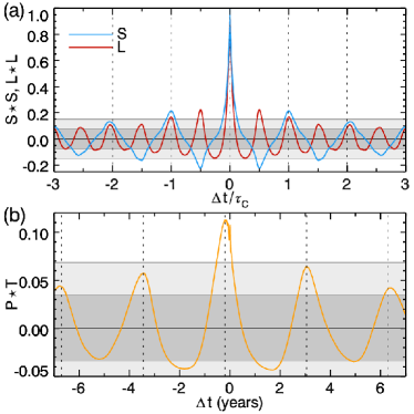
Figure 1.— (a) Volume-averaged temporal auto-correlation of toroidal magnetic energy generation by mean shear ($\mathrm{S}=\lambda\langle\mathbf{B}_{P}\rangle\bm{\cdot}\bm{\nabla}\langle\Omega\rangle$, blue curve) and the same for the mean Lorentz force impacting the mean angular velocity ($\mathrm{L}_{\phi}$, red curve) plotted against temporal lags $\Delta\mathrm{t}$ normalized by the polarity cycle period $\tau_{C}=6.2$ years. Confidence intervals are shown as shaded gray regions, with the 67% interval in darker gray and 95% in lighter gray. (b) Cross-correlation of the mean poloidal energy production ($\mathrm{P}=\mathbf{B}_{P}\bm{\cdot}\bm{\nabla}\bm{\times}\mathcal{E}^{\prime}_{\phi}$) through the fluctuating EMF and the toroidal magnetic energy production due to the mean shear ($\mathrm{T}=\langle B_{\phi}\rangle S$), showing the nonlinear dynamo wave character of the solution.

The dynamical coupling of azimuthally-averaged magnetic fields $\langle\mathbf{B}\rangle$ and the mean angular velocity $\langle\Omega\rangle$ (Figure 3(b)) plays a crucial role in regulating the cycle, though it alone cannot be the sole actor as is well known from Cowling’s anti-dynamo theorem. The significant anti-correlation of $\langle B_{\phi}\rangle$ and angular velocity variations $\langle\Delta\Omega\rangle$ during reversals becomes apparent when comparing Figures 1(c) and 3(c), revealing the strong nonlinear coupling of the magnetic field and the large-scale flows. The dynamics that couples these two fields is the toroidal field generation through the mean shear ($\mathrm{S}=\lambda\langle\mathbf{B}_{P}\rangle\bm{\cdot}\bm{\nabla}\langle\Omega\rangle$, with $\langle\mathbf{B}_{P}\rangle$ the mean poloidal field) and the mean azimuthal Lorentz-force ($L_{\phi}=\bm{\hat{\phi}\cdot}\langle\mathbf{J}\rangle\bm{\times}\langle\mathbf{B}\rangle$), which acts to decrease $\langle\Omega\rangle$. The auto-correlation of each of these components of the MHD system reveals that $L_{\phi}$ varies with a period corresponding to the magnetic energy cycle, whereas $\mathrm{S}$ varies on the polarity cycle period (Figure 1). It also shows the high degree of temporal self-similarity between cycles, with the auto-correlation of both quantities remaining significant with 95% confidence for a single polarity cycle and with 67% confidence for three such cycles.

Appealing to Figure 1(c), it is evident that $\mathbf{B}$ exhibits a high degree of spatial and temporal self-similarity, though with reversing polarity. Thus the period apparent in the auto-correlation for $L_{\phi}$ might be expected. Furthermore, if we simply let $\langle\mathbf{B}\rangle\approx\mathbf{B}_{0}(r,\theta)\exp(i\omega_{C}t)$, the Lorentz forces could be characterized very roughly as $L_{\phi}\propto{L_{\phi}}_{,0}\exp(i\omega_{L}t)\sim\mathbf{B}_{0}\cdot\mathbf{B}_{0}/\ell\exp(2i\omega_{C}t)$, with cycle frequency $\omega_{C}=2\pi/\tau_{C}$ and some length scale $\ell$. Hence, the magnetic energy or Lorentz cycle frequency $\omega_{L}=2\pi/\tau_{L}$ implies that $2\tau_{L}=\tau_{C}$. What is potentially more curious is that $\mathrm{S}$ varies on the cycle period. While Figure 3(c) might suggest a reversal in the solar-like character of the differential rotation. This in fact does not occur. Rather, the shear is significantly weakened but maintains the positive latitudinal gradient that sustains the toroidal magnetic field, which renders the sign of $\bm{\nabla}\Omega$ independent of time. Therefore, the polarity reversals in $\langle\mathbf{B}_{P}\rangle$ require that $\mathrm{S}$ vary with the polarity cycle period $\tau_{C}$.

An interval of magnetic quiescence. (a) Time-latitude diagram of $\langle B_{\phi}\rangle$ at $0.95\,\mathrm{R}\,\!\scriptscriptstyle\sun\!$ in cylindrical projection, picturing the loss and reappearance of cyclical polarity reversals as well as the lower amplitude of the wreaths. Strong positive toroidal field is shown as red, negative in blue. (b) Normalized magnetic dipole moment (red) and the quarupolar moment (blue). The quadrupole moment peaks near reversals, indicating its importance.

5. Equatorward Propagation

As with ASH and EULAG, simulations in spherical segments that employ the Pencil code also obtain regular cyclical magnetic behavior. Some of these polarity reversing solutions exhibiting equatorward propagating magnetic features (Käpylä et al., 2012), magnetic flux ejection (Warnecke et al., 2012), and 33-year magnetic polarity cycles (Warnecke, 2013). Currently, however, the mechanism for the equatorward propagation of the magnetic structures in those simulations remains unclear. Perhaps the mechanism is similar to that seen here.

The equatorward propagation of magnetic features observed in this case, as in Figures 1(c) and 4(a), arises through two mechanisms. The first process is the nonlinear feedback of the Lorentz force that acts to quench the differential rotation, disrupting the convective patterns and the shear-sustaining Reynolds stresses they possess. Since the latitudinal shear serves to build and maintain the magnetic wreaths, the latitude of peak magnetic energy corresponds to that of the greatest shear. So the region with available shear moves progressively closer to the equator as the Lorentz forces of the wreaths locally weaken the shear. Such a mechanism explains the periodic modifications of the differential rotation seen in Figure 3(c). However, it does not explain how this propagation is initiated and sustained, as one might instead expect an equilibrium to be established with the magnetic energy generation balancing the production of shear and which is further moderated by cross-equatorially magnetic flux cancellation as the distance between the wreaths declines.

There are two possibilities for the second mechanism that promotes the equatorward propagation of toroidal magnetic field structures. If we may consider the dynamo action in this case as a dynamo wave, the velocity of the dynamo wave propagation is sensitive to the gradients in the angular velocity and the kinetic helicity in the context of an $\alpha\Omega$ dynamo (e.g., Parker, 1955; Yoshimura, 1975). A simple analysis indicates that near and poleward of the edge of the low-latitude wreaths the sign of the Parker-Yoshimura mechanism is correct to push the dynamo wave toward the equator, but the effect is marginal elsewhere. The second possibility is that the spatial and temporal offsets between the fluctuating EMF and the mean-shear production of toroidal field leads to a nonlinear inducement to move equatorward. This mechanism relies on the concurrent movement of the turbulent production of the poloidal field that continues to destroy gradients in angular velocity through the production of toroidal magnetic through the action of the differential rotation on the renewed poloidal field. Nonetheless, the wreaths eventually lose their azimuthal coherence because of cross-equatorial flux cancellation and the lack of sufficient differential rotation to sustain them, which leads to a rapid dissemination of the remaining flux by the convection. This is evident in Figure 1(a), where at the end of each cycle the wreaths converge on the equator and their resulting destruction leads to the poleward advection of field. This advected field is of the opposite sense of the previous cycle’s polar cap and, being of greater amplitude compared to the remaining polar field, establishes the sense of the subsequent cycle’s polar field. Furthermore, in D3S, as a cycle progresses the centroid for the greatest dynamo action propagates both equatorward and downward in radius, as might be deduced from the successful reversals visible in Figure 4(b). Though, it is more evident in a time-radius diagram. Hence, the equatorial migration begun at the surface makes its way deeper into the domain as the cycle progresses.

6. Grand Minima

As with some other dynamo simulations (e.g., Brown et al., 2011; Augustson et al., 2013), there is also long-term modulation in case D3S. Figure 4 shows an interval of about 20 years where the polarity cycles are lost, though the magnetic energy cycles resulting from the nonlinear interaction of the differential rotation and the Lorentz force remains. During this period, the magnetic energy in the domain is about 25% lower, whereas the energy in the volume encompassed by the lower-latitudes is decreased by 60%. However, both the spatial and temporal coherency of the cycles are recovered after this interval and persist for the last 40 years of the 100 year-long simulation. Prior to entering this quiescent period, there was an atypical cycle with only the northern hemisphere exhibiting equatorward propagation. This cycle also exhibits a prominent loss of the equatorial anti-symmetry in its magnetic polarity. The subsequent four energy cycles do not reverse their polarity, which is especially evident in the polar regions, whereas the lower latitudes do seem to attempt such reversals.

7. Conclusions

The simulation presented here is the first to self-consistently exhibit four prominent aspects of solar magnetism: regular magnetic energy cycles during which the magnetic polarity reverses, akin to the sunspot cycle; magnetic polarity cycles with a period of 6.2 years, where the orientation of the dipole moment returns to that of the initial condition; the equatorward migration of toroidal field structures during these cycles; and quiescence after which the previous polarity cycle is recovered. Furthermore, this simulation may capture some aspects of the influence of a layer of near-surface shear, with a weak negative gradient in $\langle\Omega\rangle$ within the upper 10% of the computation domain (3% by solar radius). The magnetic energy cycles with the time scale $\tau_{C}/2$ arise through the nonlinear interaction of the differential rotation and the Lorentz force. We find that the nonlinear feedback of the Lorentz force on the differential rotation significantly reduces its role in the generation of toroidal magnetic energy. The magnetic fields further quench the differential rotation by impacting the convective angular momentum transport during the reversal. Furthermore, despite the nonlinearity of the case, there is an eligible influence of a dynamo wave in the fluctuating production of poloidal magnetic field linked to the shear-produced toroidal field. The mechanisms producing the equatorward propagation of the toroidal fields have been identified, with the location of the greatest latitudinal shear at a given point in the cycle and the weak negative radial shear both playing a role. This simulation has also exhibited long-lasting minimum, loosely similar to the Maunder minimum. Indeed, there is an interval covering 20% of the cycles during which the polarity does not reverse and the magnetic energy is substantially reduced. Despite rotating three times faster than the Sun and parameterizing large portions of its vast range of spatio-temporal scales, some of the features of the dynamo that may be active within the Sun’s interior have been realized in this global-scale ASH simulation.

References

- Augustson et al. (2013) Augustson, K. C., Brun, A. S., & Toomre, J. 2013, ApJ, 778, 100
- Baliunas et al. (1996) Baliunas, S. L., Nesme-Ribes, E., Sokoloff, D., & Soon, W. H. 1996, ApJ, 460, 848
- Barnes (2007) Barnes, S. A. 2007, ApJ, 669, 1167
- Brandenburg (2009) Brandenburg, A. 2009, ApJ, 697, 1206
- Brown et al. (2010) Brown, B. P., Browning, M. K., Brun, A. S., Miesch, M. S., & Toomre, J. 2010, ApJ, 711, 424
- Brown et al. (2011) Brown, B. P., Miesch, M. S., Browning, M. K., Brun, A. S., & Toomre, J. 2011, ApJ, 731, 69
- Browning et al. (2006) Browning, M. K., Miesch, M. S., Brun, A. S., & Toomre, J. 2006, ApJ, 648, L157
- Brun et al. (2004) Brun, A. S., Miesch, M. S., & Toomre, J. 2004, ApJ, 614, 1073
- Charbonneau (2013) Charbonneau, P. 2013, Journal of Physics Conference Series, 440, 012014
- Clune et al. (1999) Clune, T. L., Elliott, J. R., Miesch, M. S., Toomre, J., & Glatzmaier, G. A. 1999, Parallel Computing, 25, 361
- Fan et al. (2013) Fan, Y., Featherstone, N., & Fang, F. 2013, ArXiv e-prints
- Fares et al. (2013) Fares, R., Moutou, C., Donati, J.-F., et al. 2013, MNRAS
- Favata et al. (2008) Favata, F., Micela, G., Orlando, S., et al. 2008, A&A, 490, 1121
- Featherstone et al. (2013) Featherstone, N. A., Miesch, M. S., Brun, A.-S., & Toomre, J. 2013, J. Comp. Phys.
- Ghizaru et al. (2010) Ghizaru, M., Charbonneau, P., & Smolarkiewicz, P. K. 2010, ApJ, 715, L133
- Gilman (1983) Gilman, P. A. 1983, ApJS, 53, 243
- Glatzmaier (1985) Glatzmaier, G. A. 1985, ApJ, 291, 300
- Gleissberg (1939) Gleissberg, W. 1939, The Observatory, 62, 158
- Hathaway (2010) Hathaway, D. H. 2010, Living Reviews in Solar Physics, 7, 1
- Hempelmann et al. (1996) Hempelmann, A., Schmitt, J. H. M. M., & Stȩpień, K. 1996, A&A, 305, 284
- Jouve et al. (2010) Jouve, L., Brown, B. P., & Brun, A. S. 2010, A&A, 509, A32
- Käpylä et al. (2012) Käpylä, P. J., Mantere, M. J., & Brandenburg, A. 2012, ApJ, 755, L22
- Leighton (1969) Leighton, R. B. 1969, ApJ, 156, 1
- Malkus & Proctor (1975) Malkus, W. V. R., & Proctor, M. R. E. 1975, Journal of Fluid Mechanics, 67, 417
- Malyshkin & Boldyrev (2010) Malyshkin, L. M., & Boldyrev, S. 2010, Physical Review Letters, 105, 215002
- Mathur et al. (2013) Mathur, S., García, R. A., Morgenthaler, A., et al. 2013, A&A, 550, A32
- Metcalfe et al. (2010) Metcalfe, T. S., Basu, S., Henry, T. J., et al. 2010, ApJ, 723, L213
- Miesch et al. (2000) Miesch, M. S., Elliott, J. R., Toomre, J., et al. 2000, ApJ, 532, 593
- Morgenthaler et al. (2011) Morgenthaler, A., Petit, P., Morin, J., et al. 2011, Astronomische Nachrichten, 332, 866
- Nelson et al. (2013a) Nelson, N. J., Brown, B. P., Brun, A. S., Miesch, M. S., & Toomre, J. 2013a, ApJ, 762, 73
- Nelson et al. (2013b) Nelson, N. J., Brown, B. P., Sacha Brun, A., Miesch, M. S., & Toomre, J. 2013b, Sol. Phys., 20
- Parker (1955) Parker, E. N. 1955, ApJ, 122, 293
- Parker (1977) —. 1977, ARA&A, 15, 45
- Parker (1987) —. 1987, ApJ, 312, 868
- Parker (1993) —. 1993, ApJ, 408, 707
- Ponty et al. (2005) Ponty, Y., Mininni, P. D., Montgomery, D. C., et al. 2005, Physical Review Letters, 94, 164502
- Racine et al. (2011) Racine, É., Charbonneau, P., Ghizaru, M., Bouchat, A., & Smolarkiewicz, P. K. 2011, ApJ, 735, 46
- Rempel et al. (2009) Rempel, M., Schüssler, M., & Knölker, M. 2009, ApJ, 691, 640
- Saar (2009) Saar, S. H. 2009, in Astronomical Society of the Pacific Conference Series, Vol. 416, Solar-Stellar Dynamos as Revealed by Helio- and Asteroseismology: GONG 2008/SOHO 21, ed. M. Dikpati, T. Arentoft, I. González Hernández, C. Lindsey, & F. Hill, 375
- Schekochihin et al. (2007) Schekochihin, A. A., Iskakov, A. B., Cowley, S. C., et al. 2007, New Journal of Physics, 9, 300
- Steenbeck & Krause (1969) Steenbeck, M., & Krause, F. 1969, Astronomische Nachrichten, 291, 49
- Stenflo & Kosovichev (2012) Stenflo, J. O., & Kosovichev, A. G. 2012, ApJ, 745, 129
- Usoskin (2013) Usoskin, I. G. 2013, Living Reviews in Solar Physics, 10, 1
- Warnecke (2013) Warnecke, J. 2013, PhD thesis, University of Stockholm
- Warnecke et al. (2012) Warnecke, J., Käpylä, P. J., Mantere, M. J., & Brandenburg, A. 2012, Sol. Phys., 280, 299
- Yoshimura (1975) Yoshimura, H. 1975, ApJ, 201, 740