Local Fourier analysis of multigrid methods with polynomial smoothers and aggressive coarsening

Abstract

We focus on the study of multigrid methods with aggressive coarsening and polynomial smoothers for the solution of the linear systems corresponding to finite difference/element discretizations of the Laplace equation. Using local Fourier analysis we determine automatically the optimal values for the parameters involved in defining the polynomial smoothers and achieve fast convergence of cycles with aggressive coarsening. We also present numerical tests supporting the theoretical results and the heuristic ideas. The methods we introduce are highly parallelizable and efficient multigrid algorithms on structured and semi-structured grids in two and three spatial dimensions.

65F10, 65N22, 65N55

1 Introduction

For emerging many-core parallel architectures it has been observed that visiting the coarser levels of a multilevel hierarchy leads to a loss in performance, as measured by the percentage of peak performance achieved by the multigrid solver on such architectures. Roughly speaking, on the finer levels, computing residuals and smoothing can achieve relatively high performance, whereas on the coarser levels the performance of multigrid degrades due to the fact that fewer of the active threads are needed for computation there. These observations motivate the further study and development of multigrid methods that apply more smoothing on the finer levels together with aggressive coarsening strategies.

The use of point-wise smoothers (e.g., Jacobi and Gauss Seidel) together with aggressive coarsening in a multigrid solver has been studied using local Fourier analysis (LFA) in [20, 19] for rectangular grids and [10] for triangular grids. In these works, it has been observed that using aggressive coarsening is less efficient in terms of the total number of floating point operations than a more gradual coarsening approach, since these standard smoothing iterations are not able to effectively reduce a sufficiently large subspace of the high frequency components of the error.

However, polynomial smoothers are well suited for aggressive coarsening approach since they can be constructed to achieve a preset convergence rate on a given subspace corresponding, for example, to a subinterval of the high frequency components of the error. As shown in [17, 8, 12, 3] by using a sufficiently large degree in the polynomial approximation it is possible to guarantee prescribed damping on a preset subinterval of high frequency components. These works contain important results and provide efficient algorithms by adjusting the polynomial degree for a given coarsening ratio.

The focus of our work is on determining precisely the parameters of the polynomial smoothers, such as intervals of approximation, damping factors for high frequencies, coarsening ratios which result in best possible convergence rate. This, of course is an ambitious goal, but for semi-structured triangular and also rectangular grids this can be done. Our idea is to use the local Fourier analysis (LFA) to automatically determine the smoother and coarsening parameters which result in best performance. As we show, LFA allows us to obtain quantitative estimates of the performance of multigrid methods with polynomial smoothers of arbitrary degree and aggressive coarsening. As shown in [3, 4] polynomial smoothers result in algorithms with high degree of parallelism and outperform algorithms based on more classical relaxation methods. This is an additional advantage of the algorithms studied here as well.

The paper is organized as follows. We review some basic facts about two-grid and multigrid iterations in Section 2. Next, in Section 3 we introduce the polynomial smoothers of interest – all based on Chebyshev polynomials arising as solutions to different minimization problems – (1) appropriately shifted and scaled classical Chebyshev polynomials, (2) the so called smoothed aggregation polynomial, used as a smoother in [8], or (3) the best polynomial approximation to $\displaystyle x^{-1}$ which is proposed as a smoother in [12]. The local Fourier analysis for these polynomial smoothers, together with a two-grid LFA for aggressive coarsening are presented in Section 3.1, as are their extensions to triangular grids. Then bounds on the smoothing factors for the polynomials are calculated in Section 4. In this section we also show how to utilize the LFA results in choosing the optimal parameters for the corresponding polynomial smoother. In Section 5 we present numerical tests illustrating the findings in the previous sections and also we provide extension to triangular grids in section 5.3. Finally we draw some conclusions in Section 6.

2 Two-grid and multigrid iterations

A variational two-grid (two-level) method with one post smoothing step is defined as follows. Given an approximation $\displaystyle w\in V$ to the solution $\displaystyle u$ of the system $\displaystyle Au=f$, an update $\displaystyle v\in V$ is computed in two steps

1. $\displaystyle y=w+PA_{H}^{-1}P^{T}(f-Aw)$.

2. $\displaystyle v=y+R(f-Ay)$.

Step (1) is the coarse-grid correction iteration and step (2) is called smoothing step and the operator $\displaystyle R$ is chosen so that it is convergent in $\displaystyle A$-norm, namely $\displaystyle\parallel I-RA\parallel_{A}<1$. The corresponding error propagation operator of the two-level method is given by

$$E_{TL}=(I-RA)(I-\pi_{A}),\quad\pi_{A}=PA_{H}^{-1}P^{T}A,$$

where $\displaystyle A_{H}$ denotes the coarse-level operator, obtained by re-discretizing the problem on the coarse mesh, or, more generally, via Galerkin definition $\displaystyle A_{H}=P^{T}AP$ where $\displaystyle P$ is the prolongation matrix and $\displaystyle R$ denotes the smoothing operator. Note that if $\displaystyle\bar{R}=R+R^{T}-R^{T}AR$, then $\displaystyle\left(I-\bar{R}A\right)=(I-R^{T}A)(I-RA)$, and if $\displaystyle\bar{R}$ is SPD, then the smoother is convergent in $\displaystyle A$-norm. We will consider smoothers for which $\displaystyle R=R^{T}$ and in this case $\displaystyle\bar{R}=2R-RAR$.

The above two-level method can be easily generalized to multilevel methods by simple recursion. Suppose we already have defined the multilevel method on the coarse level, which is denoted by $\displaystyle B_{H}$ (on the coarsest level, we solve the linear system exactly, i.e. $\displaystyle B_{H}$ on the coarsest level is defined by $\displaystyle A_{H}^{-1}$), then the multilevel method on the fine level can be defined as follows:

1. $\displaystyle y=w+PB_{H}P^{T}(f-Aw)$.

2. $\displaystyle v=y+R(f-Ay)$.

It is easy to see the corresponding error propagation operator for the multilevel method is given by

$$E_{ML}=I-BA=(I-RA)(I-PB_{H}P^{T}A).$$

Note that, the multilevel method, denoted by $\displaystyle B$, is defined recursively through the multilevel method $\displaystyle B_{H}$ defined on the coarse grid.

3 Simple preconditioners and smoothers based on Chebyshev polynomials

To set the terminology, we call any SPD operator $\displaystyle R_{0}$ that approximates $\displaystyle A^{-1}$ a preconditioner. A simple example of a preconditioner $\displaystyle R_{0}$ is the inverse of the diagonal of $\displaystyle A$, i.e. $\displaystyle R_{0}=D^{-1}$. Another example is furnished by the $\displaystyle\ell_{1}$-Jacobi preconditioner introduced in [11]:

$$R_{0}=R_{\ell_{1}}=\operatorname{diag}(r_{11},r_{22},\ldots),\quad r_{ii}=1/(a_{ii}+\sum_{j\neq i}|a_{ij}|).$$

Note that $\displaystyle R_{0}$ in such case is also a convergent smoother in the terminology given above. A weighted version of $\displaystyle R_{\ell_{1}}$ can be found in [8].

Next, for any given preconditioner we can construct a convergent smoother in the following way: Given a preconditioner $\displaystyle R_{0}$, let $\displaystyle\lambda_{1}$ be a given bound on the spectral radius of $\displaystyle R_{0}A$, that is, $\displaystyle\rho(R_{0}A)\leq\lambda_{1}$ and $\displaystyle q_{\nu}(x)\in\mathcal{P}_{\nu}$ be a polynomial of degree $\displaystyle\nu$ such that

$$|1-xq_{\nu}(x)|<1,\quad\mbox{for all}\quad x\in[0,\lambda_{1}].$$ (3.1)

We then set

$$R=q_{\nu}(R_{0}A)R_{0}\quad\mbox{or equivalently}\quad R=R_{0}^{\frac{1}{2}}q_{\nu}(R_{0}^{\frac{1}{2}}AR_{0}^{\frac{1}{2}})R_{0}^{\frac{1}{2}}.$$ (3.2)

Note that this is a symmetric, and, by (3.1), a convergent smoother.

Various polynomial approximations and the resulting parallel smoothers have been designed (also in the context of aggressive coarsening), see e.g. [1, 6, 7, 12, 14, 16].

We consider three different polynomial smoothers given in (3.2). As all these are based on Chebyshev polynomials of first kind we recall the definitions of the $\displaystyle k$-th such polynomial $\displaystyle T_{k}(t)$ and the following recurrence relation

$$T_{0}(t)=1,\quad T_{1}(t)=t,\quad T_{k}(t)=2tT_{k-1}(t)-T_{k-2}(t).$$

Equivalently we can compute that

$$T_{k}(t)=\frac{1}{2}\left(t-\sqrt{t^{2}-1}\right)^{k}+\frac{1}{2}\left(t+\sqrt{t^{2}-1}\right)^{k}.$$

Clearly, $\displaystyle|T_{k}(t)|\leq 1$, $\displaystyle t\in[-1,1]$, and $\displaystyle T_{k}(t)=\pm 1$ at $\displaystyle(k+1)$ different points in $\displaystyle[-1,1]$. It is clear then that $\displaystyle|T_{k}(t)|$ is strictly monotone for $\displaystyle t\notin(-1,1)$.

We now define the three sequences of polynomials $\displaystyle\{q_{\nu}\}$ that we consider in this study. We fix $\displaystyle R_{0}$ and $\displaystyle\lambda_{1}\geq\rho(R_{0}A)$. Generally, we aim to construct a smoother $\displaystyle q_{\nu}(x)$ such that the polynomial $\displaystyle p_{\nu+1}(x)=1-xq_{\nu}(x)$ is small on the interval $\displaystyle[\lambda_{0},\lambda_{1}]$, with $\displaystyle 0\leq\lambda_{0}$. Here $\displaystyle\nu$ denotes the degree of the polynomial smoother, $\displaystyle\lambda_{1}$ is an approximation to the largest eigenvalue of $\displaystyle R_{0}A$, satisfying $\displaystyle\lambda_{1}>\rho(R_{0}A)$ and $\displaystyle\lambda_{0}$ is a parameter that can be adjusted to define the smoothing interval. In some of the cases we set $\displaystyle\lambda_{0}=\frac{\lambda_{1}}{\kappa}$, with $\displaystyle\kappa>1$, and in other cases we take $\displaystyle\lambda_{0}=0$. The smoothing factors clearly depend on the choice of $\displaystyle\lambda_{0}$. How to choose this parameter optimally is not obvious and this is discussed and addressed in our study.

The scaled and shifted classical Chebyshev polynomial solves the following minimization problem:

$$p_{\nu+1}(x)=\arg\min\{\|p\|_{\infty,[\lambda_{0},\lambda_{1}]},\quad p\in\mathcal{P}_{\nu+1},\quad\mbox{such that}\quad p(0)=1\}.$$ (3.3)

and we have then for $\displaystyle q_{\nu}(x)$:

$$q_{\nu}(x)=\frac{1-p_{\nu+1}(x)}{x},\quad p_{\nu+1}(x)=\frac{T_{\nu+1}\left(\frac{\lambda_{0}+\lambda_{1}-2x}{\lambda_{1}-\lambda_{0}}\right)}{T_{\nu+1}\left(\frac{\lambda_{0}+\lambda_{1}}{\lambda_{1}-\lambda_{0}}\right)}.$$ (3.4)

Note that $\displaystyle p_{\nu+1}(x)=1-xq_{\nu}(x)$, and from the monotonicity of $\displaystyle T_{\nu+1}(t)$ for $\displaystyle t\notin(-1,1)$ we have $\displaystyle|p_{\nu+1}(x)|<1$, for all $\displaystyle x\in[0,\lambda_{1}]$. This inequality holds independently of the choice of $\displaystyle\lambda_{0}\in[0,\lambda_{1})$. We also refer to [2, 18] for more details on these smoothers.

Using the three term recurrence relation of Chebyshev polynomials, it is straightforward to get the following identity

$$q_{\nu}(x)-q_{\nu-1}(x)=\frac{2\zeta aT_{\nu}(a)}{T_{\nu+1}(a)}(1-xq_{\nu-1}(x))+\frac{T_{\nu-1}(a)}{T_{\nu+1}(a)}(q_{\nu-1}(x)-q_{\nu-2}(x)).$$

where $\displaystyle\zeta=\frac{2}{\lambda_{1}+\lambda_{0}}$ and $\displaystyle a=\frac{\lambda_{1}+\lambda_{0}}{\lambda_{1}-\lambda_{0}}$. This identity leads to the following algorithm which computes

$$Rr=q_{\mu}(D^{-1}A)D^{-1}r.$$

Algorithm 1 Chebyshev Polynomial Preconditioning with $\displaystyle R=q_{\mu}(D^{-1}A)D^{-1}$

1:  $\displaystyle\bar{r}\leftarrow D^{-1}r$,

2:  $\displaystyle v_{0}\leftarrow a\bar{r}$,

3:  $\displaystyle v_{1}\leftarrow\frac{4\zeta a^{2}}{2a^{2}-1}\bar{r}-\frac{2\zeta^{2}a^{2}}{2a^{2}-1}D^{-1}A\bar{r}$,

4:  for $\displaystyle j=2,3,\ldots,m$ do

5:     $\displaystyle\bar{r}_{j-1}\leftarrow D^{-1}(r-Av_{j-1})$,

6:     $\displaystyle v_{j}=v_{j-1}+\frac{T_{j-1}(a)}{T_{j+1}(a)}(v_{j-1}-v_{j-2})+\frac{2\zeta aT_{j}(a)}{T_{j+1}(a)}\bar{r}_{j-1}$.

7:  end for

To define the smoothed aggregation polynomial smoother (see [8]), we use a minimization problem to define first $\displaystyle p_{\nu+1}(x)$:

$$p_{\nu+1}=\arg\min\{\|p\sqrt{x}\|_{\infty,[0,\lambda_{1}]},\quad p\in\mathcal{P}_{\nu+1},\quad\mbox{such that}\quad p(0)=1\}.$$ (3.5)

The smoothed aggregation polynomial $\displaystyle q_{\nu}$ is then defined as follows:

$$q_{\nu}(x)=\frac{1-p_{\nu+1}(x)}{x},\quad p_{\nu+1}(x)=(-1)^{\nu}\bigg{(}\frac{1}{2\nu+3}\bigg{)}\bigg{(}\frac{\sqrt{\lambda_{1}}}{\sqrt{x}}\bigg{)}T_{2\nu+3}\bigg{(}\frac{\sqrt{x}}{\sqrt{\lambda_{1}}}\bigg{)}.$$ (3.6)

Note that this formulation does not require the parameter $\displaystyle\lambda_{0}$. We refer to [16, 8, 7] for additional properties of this smoother.

Finally, we mention the smoother based on the best polynomial approximation to $\displaystyle 1/x$ in uniform norm from [12]. The minimization problem now directly defines $\displaystyle q_{\nu}(x)$ and

$$q_{\nu}(x)=\arg\min\{\|x^{-1}-p\|_{\infty,[\lambda_{0},\lambda_{1}]},\quad p\in\mathcal{P}_{\nu}\}.$$ (3.7)

Introducing $\displaystyle p_{\nu+1}(x)$ as in the previous cases, we note that this formulation thus biases the approximation to small values of $\displaystyle x$. The polynomial $\displaystyle q_{\nu}(x)$ is computed using three-term recurrence relation. For details on this polynomial and its implementation we refer to [12].

3.1 Local Fourier analysis for polynomial smoothers

We now describe briefly the technique known as Local Fourier Analysis (LFA), introduced by Brandt in [5]. This technique is considered to be a useful tool in providing quantitative convergence estimates for idealized multigrid algorithms. Such estimates can be rigorously justified in cases when the boundary conditions are periodic. It is also known that for structured or semi-structured grids the LFA provides accurate predictions for the asymptotic convergence rates of multigrid methods for problems with other types of boundary conditions as well. The analysis is based on the Discrete Fourier transform, and a good introduction to such analysis is found in the monographs by Trottenberg et al. [15], and Wienands and Joppich [19].

The main idea of the LFA is to formally extend all multigrid components to an infinite grid, neglecting the boundary conditions, and analyze discrete linear operators with constant coefficients. In this way, the eigenfunctions of such operators are the eigenfunctions of the shift operators, namely, $\displaystyle S_{\pm h}\varphi=\varphi(\cdot\pm h)$, called Fourier components. If we assume that the error is a linear combination of the Fourier components, then the behavior of a multigrid algorithm can be studied by looking at the reduction on each one of these components. Although this analysis seems to be somewhat heuristic, its practical value has been widely recognized. In general, the LFA does not only provide accurate asymptotic convergence rates, but also provides the means to select optimal components for the multigrid algorithm.

In this section, we present a suitable local Fourier analysis technique to derive quantitative estimates for the convergence of multigrid methods with polynomial smoothers and aggressive coarsening. In particular, a smoothing analysis for polynomial smoothers and a two-level analysis by considering aggressive coarsening from a grid with step-size $\displaystyle h$ to a coarse-grid of size $\displaystyle 2^{k}h$, are introduced next. We begin by setting up the LFA framework. We extend the discrete problem $\displaystyle A_{h}u_{h}=f_{h}$ to an infinite grid

$$\Omega_{h}=\{{\mathbf{x}}=(x_{1},x_{2})\,|\,x_{i}=k_{i}h_{i},\;k_{i}\in{\mathbb{Z}},\ i=1,2\},$$ (3.8)

where $\displaystyle{\bf h}=(h_{1},h_{2})$ is the grid spacing. From the definition of the operators on $\displaystyle\Omega_{h}$, the discrete solution, its current approximation and the corresponding error or residual can be represented by formal linear combinations of the Fourier modes: $\displaystyle\varphi_{h}({\bm{\theta}},{\mathbf{x}})={\rm e}^{i\theta_{1}x_{1}}\,{\rm e}^{i\theta_{2}x_{2}}$, with $\displaystyle{\mathbf{x}}\in\Omega_{h}$, and $\displaystyle{\bm{\theta}}=(\theta_{1},\theta_{2})\in{\bm{\Theta}}_{h}=(-\pi/h_{1},\pi/h_{1}]\times(-\pi/h_{2},\pi/h_{2}]$. These grid functions form a unitary basis for the space of bounded functions on the infinite grid, and define the Fourier space

$${\mathcal{F}}(\Omega_{h}):=span\{\varphi_{h}({\bm{\theta},\cdot})\,|\,{\bm{\theta}}\in{\bm{\Theta}}_{h}\}.$$

In this way, the behavior of the multigrid method can be analyzed by evaluating the error reduction associated with a particular multigrid component on the Fourier modes. Clearly, the discrete operator, and, also the discrete error transfer operator have simpler form when expressed in the Fourier basis. For instance, the symbol of $\displaystyle A_{h}$, denoted by $\displaystyle\widetilde{A}_{h}$, is typically (block) diagonal, and each diagonal element corresponds to a particular “frequency”. In what follows, we denote by $\displaystyle\widetilde{X}$ the Fourier symbol of a given operator $\displaystyle X$.

To perform a smoothing or a two-grid analysis, we distinguish high- and low-frequency components on $\displaystyle\Omega_{h}$. The classification of “high” and “low” here is done with respect to the coarse grid, since some Fourier components are not “visible” on the coarse grid. Usually such “invisible” modes are zero at the coarse grid degrees of freedom, or, they are orthogonal (in an appropriate scalar product) to all Fourier modes corresponding to the coarser grid.

Here, we consider aggressive coarsening techniques and the coarse grid is denoted by $\displaystyle\Omega_{2^{k}h}$, with $\displaystyle k$ characterizing how “aggressive” the coarsening is. Then, the range of frequencies with respect to this coarse grid is defined as

$$\begin{array}[]{rcl}\mbox{all frequencies:}&&{\bm{\Theta}}_{h}=(-\pi/h_{1},\pi/h_{1}]\times(-\pi/h_{2},\pi/h_{2}],\\ \mbox{low frequencies:}&&{\bm{\Theta}}_{2^{k}h}=(-\pi/(2^{k}h_{1}),\pi/(2^{k}h_{1})]\times(-\pi/(2^{k}h_{2}),\pi/(2^{k}h_{2})],\\ \mbox{high frequencies:}&&{\bm{\Theta}}_{h}\backslash{\bm{\Theta}}_{2^{k}h}.\end{array}$$ (3.9)

In order to investigate the action of the smoothing operator on the high-frequency error components we use a technique known as smoothing analysis.

We consider a splitting of the discrete operator $\displaystyle A_{h}=A_{h}^{+}+A_{h}^{-}$, where the splitting defines the smoothing iteration: with a given initial guess $\displaystyle u_{h,0}$ we define $\displaystyle u_{h,k+1}$ in terms of $\displaystyle u_{h,k}$ as follows:

$$\bm{u}_{h,k+1}=\bm{u}_{h,k}+[A_{h}^{+}]^{-1}(f-A_{h}u_{h,k}).$$

Smoothing analysis can be performed for many choices (symmetric or non-symmetric) of $\displaystyle[A_{h}^{+}]^{-1}$, but to tie this to our earlier discussion, the smoothers we are interested in are given by $\displaystyle R_{0}=[A_{h}^{+}]^{-1}$ in (3.2) with SPD $\displaystyle A_{h}^{+}$. For example, such smoothers are the Jacobi method, i.e. $\displaystyle A_{h}^{+}=D=\text{diag}(A_{h})$ and the $\displaystyle\ell_{1}$-smoother mentioned earlier.

For the polynomial smoothers, which are of interest here, the error propagation operator is

$$S_{h}=I_{h}-p_{m}(X)X,\quad\mbox{with}\quad X=[A_{h}^{+}]^{-1}A_{h}$$ (3.10)

where $\displaystyle p_{m}$ is a polynomial of degree $\displaystyle m$, positive on the spectrum of $\displaystyle A_{h}$. Since Fourier modes are eigenfunctions of the smoothing operator, we can estimate the smoothing factor of $\displaystyle S_{h}$, i.e. the error reduction in the space of high-frequencies $\displaystyle\widetilde{S}_{h}({\bm{\theta}})$, as follows

$$\mu=\sup_{{\bm{\Theta}}_{h}\backslash{\bm{\Theta}}_{2^{k}h}}|\widetilde{S}_{h}^{\nu}({\bm{\theta}})|,$$ (3.11)

where $\displaystyle\nu$ denotes the number of iterations of the relaxation process.

3.2 Two-grid LFA for aggressive coarsening

The basis for the efficient performance of a multigrid method is the interplay between the smoothing and the coarse-grid correction parts of the algorithm. Thus, to get more insight in the behavior of a multigrid algorithm, it is convenient to perform at least a two-grid analysis which takes into account the influence of the components involved in the coarse-grid correction. This is even more important when aggressive coarsening strategies are applied, since the smoother should be chosen according to the factor we are coarsening with. With this purpose, in this section we present a two-grid local Fourier analysis which considers an aggressive coarsening strategy from a grid with step-size $\displaystyle h$ to a grid with step-size $\displaystyle 2^{k}h$.

To perform this analysis, we consider the fine- and coarse-grids $\displaystyle\Omega_{h}$ and $\displaystyle\Omega_{2^{k}h}$, respectively. It is well known that in the transition from the fine- to the coarse-grid, each low-frequency is coupled with several high-frequencies. In particular, for an arbitrary $\displaystyle k$, each low-frequency $\displaystyle{\bm{\theta}}\in\bm{\Theta}_{2^{k}h}=(-\pi/(2^{k}h),\pi/(2^{k}h)]\times(-\pi/(2^{k}h),\pi/(2^{k}h)]$ is coupled with $\displaystyle 4^{k}-1$ high-frequencies by the coarse-grid correction operator. Because of this, the Fourier space can be subdivided into the corresponding $\displaystyle 4^{k}-$dimensional subspaces $\displaystyle{\mathcal{F}}^{2^{k}h}({\bm{\theta}})$ which are generated by the Fourier modes associated with these $\displaystyle 4^{k}$ frequencies, in the way that $\displaystyle\displaystyle{\mathcal{F}}(\Omega_{h})=\bigoplus_{{\bm{\theta}}\in\bm{\Theta}_{2^{k}h}}{\mathcal{F}}^{2^{k}h}({\bm{\theta}})$. Therefore, a block-matrix representation of the two-grid operator on the Fourier space can be obtained, which simplifies the computation of the spectral radius of the iteration matrix of the method, since the result should be the maximum of the spectral radius of the corresponding blocks.

Let $\displaystyle B_{h}^{2^{k}h}$ be the error propagation matrix of the considered two-grid method, that is, $\displaystyle e_{h}^{m+1}=B_{h}^{2^{k}h}e_{h}^{m}$, given by

$$B_{h}^{2^{k}h}=S_{h}^{\nu_{2}}C_{h}^{2^{k}h}S_{h}^{\nu_{1}}=S_{h}^{\nu_{2}}(I_{h}-P^{h}_{2^{k}h}(A_{2^{k}h})^{-1}R_{h}^{2^{k}h}A_{h})S_{h}^{\nu_{1}},$$ (3.12)

where $\displaystyle S_{h}$ is the iteration matrix associated with the smoother, $\displaystyle\nu_{1}$ , $\displaystyle\nu_{2}$ are, respectively, the number of pre- and post-smoothing steps, and $\displaystyle C_{h}^{2^{k}h}$ is the coarse-grid correction operator, mainly composed of the inter-grid transfer operators: $\displaystyle P^{h}_{2^{k}h}$, $\displaystyle R_{h}^{2^{k}h}$ restriction and prolongation, respectively, and the discrete operators $\displaystyle A_{h}$, $\displaystyle A_{2^{k}h}$ on the fine and coarse grids, respectively. For standard relaxation schemes and, in particular, for the polynomial smoothers used here the two-grid operator $\displaystyle B_{h}^{2^{k}h}$ leaves invariant the subspaces $\displaystyle{\mathcal{F}}^{2^{k}h}({\bm{\theta}})$. As a consequence this operator can be represented by a block-diagonal matrix, consisting of $\displaystyle(4^{k}\times 4^{k})-$blocks, denoted by

$$\widetilde{B}_{h}^{2^{k}h}({\bm{\theta}})=(\widetilde{S}_{h}({\bm{\theta}}))^{\nu_{2}}\widetilde{C}_{h}^{2^{k}h}({\bm{\theta}})(\widetilde{S}_{h}({\bm{\theta}}))^{\nu_{1}}.$$

Here, $\displaystyle{\bm{\theta}}\in\bm{\Theta}_{2^{k}h}$, $\displaystyle\widetilde{S}_{h}({\bm{\theta}})$, and $\displaystyle\widetilde{C}_{h}^{2^{k}h}({\bm{\theta}})$ are the block-matrix representations in the subspaces $\displaystyle{\mathcal{F}}^{2^{k}h}({\bm{\theta}})$ of the smoother and the coarse-grid correction operator. The latter is computed from the Fourier representations of the coarse-grid correction, namely,

$$\widetilde{C}_{h}^{2^{k}h}=\widetilde{I}_{h}-\widetilde{P}^{h}_{2^{k}h}(\widetilde{A}_{2^{k}h})^{-1}\widetilde{R}_{h}^{2^{k}h}\widetilde{A}_{h}.$$ (3.13)

Now, the local Fourier analysis prediction for the asymptotic two-grid convergence factor of the method can be determined as:

$$\rho=\rho(B_{h}^{2^{k}h})=\max_{{\bm{\theta}}\in\bm{\Theta}_{2^{k}h}}\rho(\widetilde{B}_{h}^{2^{k}h}({\bm{\theta}})).$$ (3.14)

3.3 Extension to triangular grids

To analyze the influence of grid-geometry on the behavior of the multigrid method, in this section we extend the ideas to triangular grids. We consider the discretization of the Laplace operator by linear finite elements on a regular triangulation of a general triangle.

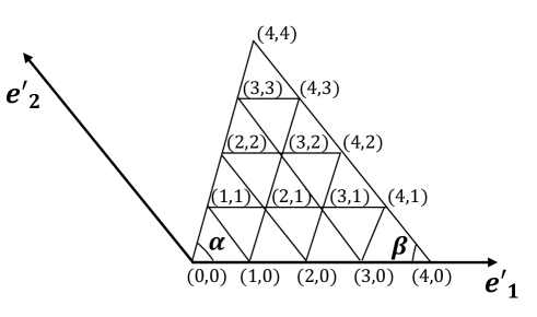
Figure 3.1: Basis in $\displaystyle{\mathbb{R}}^{2}$ fitting the geometry of a triangular grid characterized by two angles, and local enumeration for the regular grid obtained after two refinement levels.

This triangular grid is characterized by two angles $\displaystyle\alpha$ and $\displaystyle\beta$ and a local enumeration with double index is fixed by considering a unitary basis of $\displaystyle{\mathbb{R}}^{2}$, $\displaystyle\{{\mathbf{e}}_{1}^{\prime},{\mathbf{e}}_{2}^{\prime}\}$, fitting the geometry of the triangular grid (see Figure 3.1). We fix the axis-orientation $\displaystyle\{{\mathbf{e}}_{1}^{\prime},{\mathbf{e}}_{2}^{\prime}\}$, the corresponding enumeration of vertices as in Figure 3.1, and we set $\displaystyle\gamma=\pi-\alpha-\beta$. The stencil form of the discrete operator then reads (see, e.g. [13, pp. 189–190])

$$A_{h}=\displaystyle\frac{\cot\alpha+\cot\beta}{h^{2}}\begin{bmatrix}0&-\cot\alpha&-\cot\beta\\ -\cot\gamma&2(\cot\alpha+\cot\beta+\cot\gamma)&-\cot\gamma\\ -\cot\beta&-\cot\alpha&0\end{bmatrix}.$$ (3.15)

Following [9], the local Fourier analysis applied to discretizations on rectangular grids, can be extended to discretizations on triangulations. The key to carrying out this generalization is to define a new two-dimensional Fourier transform using non-orthogonal bases. More precisely, we pick a spatial basis that fits the structure of the grid (see Figure 3.1) and we chose its reciprocal basis in the frequency space. In this way LFA on triangular grids is performed similarly as on rectangular grids.

4 Bounds via local Fourier analysis

From the considerations in Section 3 we know that to construct smoothers based on scaled Chebyshev polynomials or based on the $\displaystyle\text{BA}_{1/x}$polynomial we need to specify the interval $\displaystyle[\lambda_{0},\lambda_{1}]$. On this interval, as mentioned earlier the polynomials have optimal properties and solve different minimization problems.

In this section, we describe briefly how to optimize the choice of $\displaystyle\lambda_{0}$ used in defining $\displaystyle{\mathcal{Q}}_{m}((A_{h}^{+})^{-1}A_{h})$. One simple choice is to use LFA for $\displaystyle(\widetilde{A}_{h}^{+}(\bm{\theta}))^{-1}\widetilde{A}_{h}(\bm{\theta})$, and define $\displaystyle\lambda_{0}$ and $\displaystyle\lambda_{1}$ as

$$\lambda_{0}=\min_{\theta\in{\bm{\Theta}}_{h}\backslash{\bm{\Theta}}_{2^{k}h}}|(\widetilde{A}_{h}^{+}(\bm{\theta}))^{-1}\widetilde{A}_{h}(\bm{\theta})|,\qquad\lambda_{1}=\max_{\theta\in{\bm{\Theta}}_{h}\backslash{\bm{\Theta}}_{2^{k}h}}|(\widetilde{A}_{h}^{+}(\bm{\theta}))^{-1}\widetilde{A}_{h}(\bm{\theta})|.$$ (4.1)

This is a good choice, but is not optimal, as is evident from the numerical results presented later. From the properties of the classical Chebyshev polynomial smoothers and the $\displaystyle\text{BA}_{1/x}$smoother introduced in §3 we see that two parameters, $\displaystyle\lambda_{0}$ and $\displaystyle\lambda_{1}$, are used to define the smoother. Since we would like to have scaling invariant smoothers we can fix one of these parameters. For reasons which are evident from the analysis provided in [2, 18] for the scaled Chebyshev smoother and [12] for the smoother using the best approximation to $\displaystyle\frac{1}{x}$, the parameter that we fix is $\displaystyle\lambda_{1}$. To optimize the performance of the smoother or the two grid method, we try to adjust $\displaystyle\lambda_{0}$ in order to achieve one of the following goals:

• get better smoothing properties, that is, minimize $\displaystyle|\widetilde{S}_{h}(\bm{\theta})|$ for $\displaystyle\bm{\theta}\in\bm{\Theta}_{h}\setminus\bm{\Theta}_{2^{k}h}$ (high frequency as defined in (3.9)) to compensate for aggressive coarsening.

• get the best possible two grid rate of convergence, namely, minimize $\displaystyle|\widetilde{B}_{h}^{2^{k}h}(\bm{\theta})|$ for $\displaystyle\bm{\theta}\in\bm{\Theta}_{h}$.

We find an optimal value of $\displaystyle\lambda_{0}$ iteratively, choosing as initial guess the values given in (4.1). This can be done as explained in the next section.

4.1 Optimal choice of $\displaystyle\lambda_{0}$

We now provide several of the relevant properties on this polynomial smoother and discuss the choice of $\displaystyle\lambda_{0}$ for smoothers based on the polynomial of best approximation of $\displaystyle x^{-1}$. For the estimates and identities used below, we refer to [12]. Let $\displaystyle\lambda_{0}>0$ be any estimate of the minimal eigenvalue of $\displaystyle[A_{h}^{+}]^{-1}A_{h}$, for example $\displaystyle\lambda_{0}=\lambda_{1}/\kappa$, for some $\displaystyle\kappa>1$.

We now discuss the restrictions on the polynomial degree imposed by the requirement that the smoother has certain error reduction and also the requirement that the polynomial is positive on $\displaystyle(0,\lambda_{1}]$ (and as a consequence the matrix polynomial will be positive definite). Further, let

$$\displaystyle E_{m}:=\max_{x\in[\lambda_{0},\lambda_{1}]}|1-xp_{m}(x)|=\max_{x\in[\lambda_{0},\lambda_{1}]}x\cdot\left|\frac{1}{x}-p_{m}(x)\right|.$$

As $\displaystyle\lambda_{1}$ is a point of Chebyshev alternance, [12, Theorem 2.1 and Equation (2.2)], for the error of approximation $\displaystyle E_{m}$ we have

$$\displaystyle E_{m}=\lambda_{1}\left|\frac{1}{\lambda_{1}}-p_{m}(\lambda_{1})\right|=\left[\frac{2\lambda_{1}}{\lambda_{1}-\lambda_{0}}\right]\cdot\left[\frac{\delta^{m}}{a^{2}-1}\right]=\frac{2\kappa\delta^{m}}{(\kappa-1)(a^{2}-1)}.$$

Here, we have denoted

$$\kappa=\frac{\lambda_{1}}{\lambda_{0}},\quad\quad\delta=\frac{\sqrt{\kappa}-1}{\sqrt{\kappa}+1},\quad a=\frac{\kappa+1}{\kappa-1}.$$

Computing the error $\displaystyle E_{m}$ then gives

$$E_{m}=\frac{\delta^{m}(\kappa-1)}{2}.$$ (4.2)

Regarding the positivity, $\displaystyle p_{m}(\lambda_{1})>0$, a sufficient condition (and also necessary condition in many cases) is that $\displaystyle\frac{1}{\lambda_{1}}-E_{m}>0$. Thus, we need to find the smallest $\displaystyle m$ such that both $\displaystyle E_{m}<\rho$, for a given $\displaystyle\rho$, and $\displaystyle p_{m}(\lambda_{1})>0$. We then have that the polynomial is positive if

$$\displaystyle\frac{\delta^{m}(\kappa-1)}{2}\leq\frac{1}{\lambda_{1}}\quad\Rightarrow\quad\delta^{m}\leq\frac{2}{\lambda_{1}(\kappa-1)}.$$

We note that from this it follows that $\displaystyle R=p_{m}(A)$ and hence $\displaystyle\bar{R}$ are symmetric and positive definite, implying that the smoother is convergent in $\displaystyle A$-norm.

Also, a straightforward calculation shows that if we want a damping factor less than $\displaystyle\rho$ on the interval $\displaystyle[\lambda_{0},\lambda_{1}]$, we have

$$\displaystyle\frac{\delta^{m}(\kappa-1)}{2}\leq\rho\quad\Rightarrow\quad\delta^{m}\leq\frac{2\rho}{\kappa-1}.$$

Finally, the minimal $\displaystyle m$ that will have the desired properties satisfies

$$m\geq\frac{1}{|\log\delta|}\max\left\{\left|\log\frac{2\rho}{\kappa-1}\right|,\left|\log\frac{2}{\lambda_{1}(\kappa-1)}\right|\right\}.$$ (4.3)

Recall that $\displaystyle\lambda_{1}$ is fixed, and, hence, both $\displaystyle\kappa$ and the polynomial degree $\displaystyle m$ are determined by $\displaystyle\lambda_{0}$. In short, once we choose $\displaystyle\lambda_{0}$ we can calculate the degree of the polynomial so that the resulting smoother has a guaranteed convergence rate. This result is of interest in the context of aggressive coarsening since it allows to choose $\displaystyle\lambda_{0}$ in accordance with the coarsening ratio and the smoothing rate. Choosing $\displaystyle\lambda_{0}$ to optimize these two parameters naturally leads to computationally optimal methods.

Since the convergence rate of the polynomial smoother is determined by $\displaystyle\max_{x\in[\lambda_{0},\lambda_{1}]}|1-xp_{m}(x)|$, the choice of $\displaystyle\lambda_{0}$ using LFA (see (4.1)) does not guarantee the optimal convergence rate of the polynomial smoother. Instead, we consider fixing $\displaystyle\lambda_{1}$ and the polynomial degree $\displaystyle m$, and finding the best lower bound, $\displaystyle\lambda_{0}^{*}$, that solves the following min-max problem:

$$\min_{\lambda\in[\lambda_{0},\lambda_{1}]}\max_{x\in[\lambda_{0},\lambda_{1}]}|1-xp_{m}(x;\lambda)|\longrightarrow\lambda_{0}^{*},$$ (4.4)

where $\displaystyle p_{m}(x;\lambda)$ denote the best approximation of $\displaystyle 1/x$ on the interval $\displaystyle[\lambda,\lambda_{1}]$. Next we will explain how to solve this minimization problem and, therefore, obtain the optimal $\displaystyle\lambda_{0}^{*}$. First, the following lemma shows that the $\displaystyle|1-xp_{m}(x;\lambda)|$, $\displaystyle\lambda\in[\lambda_{0},\lambda_{1}]$ achieves its maximum at the end points $\displaystyle\lambda_{0}$ or $\displaystyle\lambda_{1}$.

Lemma 4.1.

If $\displaystyle\lambda\in[\lambda_{0},\lambda_{1}]$, and $\displaystyle p_{m}(x;\lambda)$ is the best polynomial approximation to $\displaystyle 1/x$ on $\displaystyle[\lambda,\lambda_{1}]$, then

$$\max_{x\in[\lambda_{0},\lambda_{1}]}|1-xp_{m}(x,\lambda)|=\max\{|1-\lambda_{1}p_{m}(\lambda_{1};\lambda)|,|1-\lambda_{0}p_{m}(\lambda_{0};\lambda)|\}.$$ (4.5)

Proof 4.2.

We first consider $\displaystyle x\in[\lambda,\lambda_{1}]$ and since $\displaystyle p_{m}(x;\lambda)$ is the best polynomial approximation to $\displaystyle 1/x$ on $\displaystyle[\lambda,\lambda_{1}]$, we have that $\displaystyle\lambda_{1}$ is a point of Chebyshev alternance. Therefore,

$$\max_{x\in[\lambda,\lambda_{1}]}|1-xp_{m}(x;\lambda)|=|1-\lambda_{1}p_{m}(\lambda_{1};\lambda)|.$$

On the other hand, for $\displaystyle x\in[\lambda_{0},\lambda]$, as shown in [12, Lemma 3.1 and Equation (3.5)], $\displaystyle p_{m}(x;\lambda)$ is strictly decreasing on $\displaystyle(0,\lambda]$, and therefore,

$$\max_{x\in[\lambda_{0},\lambda]}|1-xp_{m}(x;\lambda)|=|1-\lambda_{0}p_{m}(\lambda_{0};\lambda)|.$$

Then (4.5) follows directly and the proof is complete.

Using Lemma 4.1, the minimization problem (4.4) can be simplified as following

$$\min_{\lambda\in[\lambda_{0},\lambda_{1}]}\max\{|1-\lambda_{1}p_{m}(\lambda_{1};\lambda)|,|1-\lambda_{0}p_{m}(\lambda_{0};\lambda)|\}.$$ (4.6)

4.2 Existence of optimal parameter

In this subsection we provide convincing evidence that an optimal $\displaystyle\lambda_{0}^{*}$ exists. We have not stated this as a theorem because we have used Mathematica to verify the positivity of a derivative in the last step of the proof below. We have the following result.

Result 4.3.

If $\displaystyle\lambda\in[\lambda_{0},\lambda_{1}]$ and $\displaystyle p_{m}(x;\lambda)$ is the best polynomial approximation to $\displaystyle 1/x$ on $\displaystyle[\lambda,\lambda_{1}]$, then there is a unique minimizer $\displaystyle\lambda_{0}^{*}$ of the minimization problem (4.4), and

$$|1-\lambda_{1}p_{m}(\lambda_{1};\lambda_{0}^{*})|=|1-\lambda_{0}p_{m}(\lambda_{0};\lambda_{0}^{*})|.$$ (4.7)

Here we outline an argument which at the last step uses a bound verified numerically. As we have observed earlier, since $\displaystyle\lambda_{1}$ is a point of Chebyshev alternance, we have

$$|1-\lambda_{1}p_{m}(\lambda_{1};\lambda)|=\frac{(\sqrt{\frac{\lambda_{1}}{\lambda}}-1)^{m}(\frac{\lambda_{1}}{\lambda}-1)}{2(\sqrt{\frac{\lambda_{1}}{\lambda}}+1)^{m}},$$

As it can be easily verified, the right side of this equation is a strictly decreasing function when $\displaystyle\lambda\in[\lambda_{0},\lambda_{1}]$.

As $\displaystyle|1-\lambda_{0}p_{m}(\lambda_{0};\lambda)|={\lambda_{0}}|1/\lambda_{0}-p_{m}(\lambda_{0};\lambda)|$, we will focus on $\displaystyle\mathcal{E}_{m}(x;\lambda)=|1/x-p_{m}(x;\lambda)|$. According to the three term recurrence of $\displaystyle p_{m}(x;\lambda)$ [12, Equation (2.13)], we have

$$p_{m+1}(x;\lambda)-p_{m}(x;\lambda)=\delta^{2}(p_{m}(x;\lambda)-p_{m-1}(x;\lambda))+c(1-xp_{m}(x;\lambda)),$$

where $\displaystyle\delta=\frac{\sqrt{\kappa}-1}{\sqrt{\kappa}+1}$ with $\displaystyle\kappa=\frac{\lambda_{1}}{\lambda}$ and $\displaystyle c=\frac{4\sqrt{\mu_{0}}\sqrt{\mu_{1}}}{(\sqrt{\mu_{0}}+\sqrt{\mu_{1}})^{2}}$ with $\displaystyle\mu_{0}=\frac{1}{\lambda_{1}}$ and $\displaystyle\mu_{1}=\frac{1}{\lambda}$. Then we have the following three term recurrence of $\displaystyle\mathcal{E}_{m}(x;\lambda)$

$$\mathcal{E}_{m+1}(x;\lambda)=2y\delta\mathcal{E}_{m}(x;\lambda)-\delta^{2}\mathcal{E}_{m-1}(x;\lambda),$$

where $\displaystyle y=\frac{1+\delta^{2}-cx}{2\delta}$. Because $\displaystyle\mathcal{E}_{m}$ satisfies the homogeneous three term recurrence relationship, we have the following explicit formula

$$\mathcal{E}_{m}(x;\lambda)=-\delta^{m}\mathcal{E}_{0}(x;\lambda)U_{m-2}(y)+\delta^{m-1}\mathcal{E}_{1}(x;\lambda)U_{m-1}(y),$$

where

$$\mathcal{E}_{0}(x;\lambda)=\frac{1}{x}-\frac{1}{2}(\mu_{0}+\mu_{1});\quad\mathcal{E}_{1}(x;\lambda)=\frac{1}{x}-\left(\frac{1}{2}(\sqrt{\mu_{0}}+\sqrt{\mu_{1}})^{2}-\mu_{0}\mu_{1}x\right).$$

Using the software package Mathematica (see the output below), we can verify that $\displaystyle\mathcal{E}_{m}(\lambda_{0};\lambda)>0$ and is a strictly increasing function when $\displaystyle\lambda\in[\lambda_{0},\lambda_{1}]$, and therefore, so is

$$|1-\lambda_{0}p_{m}(\lambda_{0};\lambda)|=\lambda_{0}\mathcal{E}_{m}(\lambda_{0};\lambda).$$

Therefore, because $\displaystyle|1-\lambda_{1}p_{m}(\lambda_{1};\lambda)|$ is strictly decreasing and $\displaystyle|1-\lambda_{0}p_{m}(\lambda_{0};\lambda)|$ is strictly increasing when $\displaystyle\lambda\in[\lambda_{0},\lambda_{1}]$, $\displaystyle\min_{\lambda\in[\lambda_{0},\lambda_{1}]}\max\{|1-\lambda_{1}p_{m}(\lambda_{1};\lambda)|,|1-\lambda_{0}p_{m}(\lambda_{0};\lambda)|\}$ has a unique minimizer $\displaystyle\lambda_{0}^{*}$ satisfying (4.7). Moreover, according to Lemma 4.1, this minimizer $\displaystyle\lambda_{0}^{*}$ is the unique minimizer of the minimization problem (4.4).

Thus, Result 4.3 and (4.7), show that to find $\displaystyle\lambda_{0}^{*}$ satisfying (4.7) we need to solve a one-dimensional nonlinear equation. This value of $\displaystyle\lambda_{0}^{*}$ results in the best convergence rate for the polynomial smoother for the given range of frequencies.

At the end of this subsection, we provide the Mathematica code which is used to verify Result 4.3. Without loss of generality, we assume that $\displaystyle\lambda_{1}=1$, introduce $\displaystyle t=\sqrt{\kappa}$, and change the formulas of $\displaystyle y$, $\displaystyle\mathcal{E}_{0}$, and $\displaystyle\mathcal{E}_{1}$ correspondingly. In the Mathematica code, we first input the variables and then compute the derivative of $\displaystyle\mathcal{E}_{m}$ with respect to $\displaystyle t$.

⬇

In[1] := delta = (t-1)/(t+1);

y = (1+t^2 - 2*t*x)/(t^2 -1);

E0 = -0.5*t^2 + ((1/x) - 0.5);

E1 = -0.5*(t+1)^2 + t^2*x + 1/x;

Em = delta^(m-1)*E1*ChebyshevU[m-1,y]

- delta^m*E0*ChebyshevU[m-2,y];

Minimize[{Em, 1$\displaystyle\leq$t$\displaystyle\leq$1/Sqrt[x], 0$\displaystyle<$x$\displaystyle\leq$1, 3$\displaystyle\leq$m}, {t, x, m}];

Out[2] = $\displaystyle\left\{3.51279\times 10^{-22},\ \{\text{t}\rightarrow 1.03272,\ \text{x}\rightarrow 0.917826,\ \text{m}\rightarrow 18.11\}\right\}$

In[3] := Maximize[{$\displaystyle\partial_{x}$(Em), 1$\displaystyle\leq$t$\displaystyle\leq$1/Sqrt[x], 0$\displaystyle<$x$\displaystyle\leq$1, 3$\displaystyle\leq$m}, {t, x, m}];

Out[4] = $\displaystyle\left\{-3.77826\times 10^{-48},\ \{\text{t}\rightarrow 1.0027,\ \text{x}\rightarrow 0.919534,\ \text{m}\rightarrow 43.6199\}\right\}$

From the output displayed above, we can see that $\displaystyle\mathcal{E}_{m}>0$ and the derivative of $\displaystyle\mathcal{E}_{m}$ with respect to $\displaystyle t$ is negative and, therefore, $\displaystyle\mathcal{E}_{m}$ is strictly decreasing, which means $\displaystyle\mathcal{E}_{m}$ is strictly increasing with respect to $\displaystyle\lambda$. This concludes the heuristic justification of Result 4.3.

5 Numerical Experiments

In this section we present numerical results on smoothing properties of the polynomial smoothers and results on two- and multi-level methods which use these smoothers in combination with aggressive coarsening strategy. When the polynomial smoother is the best polynomial approximation of $\displaystyle x^{-1}$ or the Chebyshev polynomial, the tests also include study of the behavior of the smoothers and the multigrid algorithms with respect to the parameters involved in defining these polynomial smoothers (e.g. $\displaystyle\lambda_{0}$ as discussed earlier in Section 4).

To fix ideas we consider as our model problem the Poisson equation on a domain $\displaystyle\Omega$ with homogeneous Dirichlet boundary conditions

$$\displaystyle{\mathcal{A}}u({\mathbf{x}})=-\Delta u({\mathbf{x}}) \displaystyle= \displaystyle f({\mathbf{x}}),\quad{\mathbf{x}}\in\Omega\subseteq{\mathbb{R}}^{d},\;d=2,3,$$ (5.1)

$$\displaystyle u({\mathbf{x}}) \displaystyle= \displaystyle 0,\quad{\mathbf{x}}\in\partial\Omega.$$ (5.2)

The domains $\displaystyle\Omega$ which we consider are the unit cubes in $\displaystyle{\rm I\!R}^{d}$, $\displaystyle d=2,3$ or a triangular domain in $\displaystyle{\rm I\!R}^{2}$. We group the numerical tests in this section as follows. In Section 5.1 we present results on the smoothing property of the polynomial smoothers. The two-grid and multigrid results are shown in Section 5.2 . As discretization technique on rectangular grids we use the standard $\displaystyle 5$-point finite difference discretization of problem (5.1)-(5.2). At the end we also show that our results can be easily generalized to continuous linear finite element discretizations on triangular grids (see Section 5.3, and Section 3.3). In the computations, we use bilinear interpolation for rectangular grids and linear interpolation on triangular grids.

One notation that is needed is on the corresponding cycling strategy. We call $\displaystyle k$-coarsening a coarsening procedure which results in a coarser grid size of $\displaystyle 2^{k}h$ if the size of the fine grid is $\displaystyle h$. For multigrid method with total number of levels $\displaystyle L$, this means that the grid size on level $\displaystyle\ell$ is $\displaystyle 2^{k\ell}h_{L}$ if $\displaystyle L$-th level is the finest grid level. Such coarsening is called aggressive since a coarser grid has $\displaystyle 2^{-kd}n$ degrees of freedom if the spatial dimension is $\displaystyle d$ and the fine grid has $\displaystyle n$ degrees of freedom.

5.1 Comparison of smoothing rates

The crucial role of the smoothing as one main component in a multigrid process is well known (see the classical paper by A. Brandt [5]). In fact, as shown in this pioneering work on multigrid methods, the smoothing analysis can provide a first, and often accurate, estimate on the convergence factor of the overall method.

In this section, we compare the smoothing properties of the polynomial smoothers introduced in Section 3: (a) the scaled classical Chebyshev polynomial; (b) the smoothed aggregation polynomial, denoted here with (SA); and (c) the best polynomial approximation to $\displaystyle x^{-1}$, denoted here with ($\displaystyle\text{BA}_{1/x}$). For the latter polynomial we provide two different values for the lower bound of the eigenvalue interval, $\displaystyle\lambda_{0}$: (1) the choice of $\displaystyle\lambda_{0}$ given by the LFA (see (4.1)); and (2) the optimal choice of $\displaystyle\lambda_{0}$, given in Section 4.1, and denoted by $\displaystyle\lambda_{0}^{*}$. The results for the Chebyshev polynomial smoothers are for the interval $\displaystyle[\lambda_{0},\lambda_{1}]$ with the value of $\displaystyle\lambda_{0}$ determined from (4.1). In Table 5.1, we present the smoothing factors predicted by the local Fourier analysis for these polynomial smoothers in $\displaystyle 2D$. For the LFA estimates we specify as “low frequencies” the eigenmodes corresponding to a lattice of size $\displaystyle 2^{k}h$, where $\displaystyle h$ is the fine grid mesh size. In this setting, larger values of $\displaystyle k$ correspond to more aggressive coarsening. For the case of $\displaystyle\text{BA}_{1/x}$smoother this in turn requires higher degree of the polynomial.

Table 5.1: Smoothing rate comparison of different polynomial smoothers ($\displaystyle\lambda_{1}=2$) in 2D

	Chebyshev	SA	$\displaystyle\text{BA}_{1/x}$	$\displaystyle\text{BA}_{1/x}$($\displaystyle\lambda_{0}^{*}$)	$\displaystyle\lambda_{0}$	$\displaystyle\lambda_{0}^{*}$
$\displaystyle k=1$, Degree $\displaystyle=2$	0.074	0.233	0.167	0.100	0.500	0.598
$\displaystyle k=2$, Degree $\displaystyle=6$	0.041	0.221	0.226	0.086	0.146	0.202
$\displaystyle k=3$, Degree $\displaystyle=17$	0.014	0.172	0.230	0.053	0.038	0.057

We use the same degree for the Chebyshev and also SA polynomials and we observe that the scaled Chebyshev polynomial provides the best smoothing factors for any of the choices of aggressive coarsening. Also we observe that choosing the optimal value of $\displaystyle\lambda_{0}^{*}$ for the smoothing of the $\displaystyle 1/x$ polynomial improves significantly the smoothing rate for this smoother.

Next, similar results are presented in Table 5.2 for the three-dimensional case. Again, we can draw the same conclusions since Chebyshev polynomial results in the best smoothing rates (even better than in the two-dimensional case) and the optimal choice of $\displaystyle\lambda_{0}=\lambda_{0}^{*}$ appears to be crucial to obtain good convergence factors for the $\displaystyle\text{BA}_{1/x}$smoother.

Table 5.2: Smoothing rate comparison of different polynomial smoothers ($\displaystyle\lambda_{1}=2$) in 3D

	Chebyshev	SA	$\displaystyle\text{BA}_{1/x}$	$\displaystyle\text{BA}_{1/x}$($\displaystyle\lambda_{0}^{*}$)	$\displaystyle\lambda_{0}$	$\displaystyle\lambda_{0}^{*}$
$\displaystyle k=1$, Degree $\displaystyle=3$	0.062	0.227	0.185	0.097	0.333	0.419
$\displaystyle k=2$, Degree $\displaystyle=9$	0.022	0.215	0.171	0.059	0.976	0.134
$\displaystyle k=3$, Degree $\displaystyle=22$	0.011	0.148	0.268	0.051	0.025	0.039

5.2 Multigrid cycles

While the smoothing analysis results presented in previous section give us some insight about the performance of the method, to properly study the behavior of multigrid algorithm we need to involve the coarse grid correction into the tests. We first present a two-grid analysis (LFA) which takes into account the effect of transfer operators and the rest of the components of the coarse-grid correction part of the algorithm. We report the two-grid convergence rates obtained by LFA as well as the performance of a W-cycle solver using the polynomial smoothers. We present the results for two-grid method and W-cycle for $\displaystyle 1$-coarsening, i.e. all levels are involved in the coarse grid correction and there is no skipping of levels.

Next, we show results on the behavior of multigrid V-cycles. The tests are carried out for $\displaystyle k$-coarsening strategies, with $\displaystyle k=1,2,3$, namely we study the performance of the algorithms with respect to coarsening strategy with different “aggressiveness”.

For the two- and multi-grid tests we only compare Chebyshev polynomial and $\displaystyle 1/x$ polynomial since from the previous smoothing rate tests, we can assert that these two polynomials outperform the SA polynomials as smoothers. Also all the convergence factors presented in the tables are computed with only one smoothing step.

In the tables below, we denote by $\displaystyle\rho_{LFA}$ the two-grid convergence factors predicted by LFA. The results for the $\displaystyle k$-coarsening strategies are presented in Table 5.3. In order to validate these results, we also show in this table the corresponding experimentally computed asymptotic two-grid convergence factors $\displaystyle\rho_{W}$. The lower and upper bounds of the eigenvalue interval $\displaystyle[\lambda_{0},\lambda_{1}]$ provided by the LFA are also given, together with the optimal value $\displaystyle\lambda_{0}^{*}$, computed as in (4.7), and with the minimal degree of the polynomial smoothers. We observe that according to Table 5.3 the local Fourier analysis provides sharp estimates for the convergence rates in all the cases.

Finally, we remark on the choice of parameter $\displaystyle\lambda_{0}^{*}$. As seen this choice improves the convergence factors provided by $\displaystyle\text{BA}_{1/x}$smoother. The improvement is more significant for $\displaystyle k$-coarsening with larger $\displaystyle k$. This makes the convergence rates of $\displaystyle\text{BA}_{1/x}$very close to those given by the best option, namely, the scaled and shifted classical Chebyshev polynomial.

Table 5.3: Two-grid convergence rate for different polynomial smoothers in 2D

					Chebyshev		$\displaystyle\text{BA}_{1/x}$		$\displaystyle\text{BA}_{1/x}$($\displaystyle\lambda_{0}^{*}$)
	$\displaystyle\lambda_{0}$	$\displaystyle\lambda_{0}^{*}$	$\displaystyle\lambda_{1}$	Degree	$\displaystyle\rho_{LFA}$	$\displaystyle\rho_{W}$	$\displaystyle\rho_{LFA}$	$\displaystyle\rho_{W}$	$\displaystyle\rho_{LFA}$	$\displaystyle\rho_{W}$
$\displaystyle k=1$	$\displaystyle 0.5$	$\displaystyle 0.598$	$\displaystyle 2.0$	$\displaystyle 2$	$\displaystyle 0.125$	$\displaystyle 0.126$	$\displaystyle 0.166$	$\displaystyle 0.166$	$\displaystyle 0.134$	$\displaystyle 0.134$
$\displaystyle k=2$	$\displaystyle 0.146$	$\displaystyle 0.202$	$\displaystyle 2.0$	$\displaystyle 6$	$\displaystyle 0.156$	$\displaystyle 0.155$	$\displaystyle 0.221$	$\displaystyle 0.225$	$\displaystyle 0.166$	$\displaystyle 0.165$
$\displaystyle k=3$	$\displaystyle 0.038$	$\displaystyle 0.057$	$\displaystyle 2.0$	$\displaystyle 17$	$\displaystyle 0.137$	$\displaystyle 0.137$	$\displaystyle 0.227$	$\displaystyle 0.227$	$\displaystyle 0.148$	$\displaystyle 0.149$

It is also interesting to choose a value of $\displaystyle\lambda_{0}$ (left end of the high frequency interval) which is optimal with respect to the overall two-grid convergence of the method. Note that, this is a different procedure than what we have done before: choosing $\displaystyle\lambda_{0}^{*}$ such that the smoothing factor is the best possible. This value has been computed by using the local Fourier analysis, for both Chebyshev and $\displaystyle\text{BA}_{1/x}$polynomials. More precisely, we find the optimal $\displaystyle\lambda_{0}^{*}$ not only by monitoring the convergence of the smoother, but also the convergence of the two-grid method. In Table 5.4 we present two-grid convergence factors for this case as predicted by the LFA and we also show the experimentally computed W-cycle rates. We observe results similar to the ones already discussed in Table 5.3.

Table 5.4: Two-grid convergence rate for Chebyshev and $\displaystyle\text{BA}_{1/x}$polynomial smoothers. The value of $\displaystyle\lambda_{0}$ is chosen by applying LFA for the overall convergence factor of the two-grid method.

			Chebyshev($\displaystyle\lambda_{0}^{Optimal-TL}$)			$\displaystyle\text{BA}_{1/x}$($\displaystyle\lambda_{0}^{Optimal-TG}$)
	$\displaystyle\lambda_{1}$	Degree	$\displaystyle\lambda_{0}$	$\displaystyle\rho_{LFA}$	$\displaystyle\rho_{W}$	$\displaystyle\lambda_{0}$	$\displaystyle\rho_{LFA}$	$\displaystyle\rho_{W}$
$\displaystyle k=1$	$\displaystyle 2.0$	$\displaystyle 2$	$\displaystyle 0.405$	$\displaystyle 0.111$	$\displaystyle 0.113$	$\displaystyle 0.550$	$\displaystyle 0.128$	$\displaystyle 0.128$
$\displaystyle k=2$	$\displaystyle 2.0$	$\displaystyle 6$	$\displaystyle 0.095$	$\displaystyle 0.138$	$\displaystyle 0.140$	$\displaystyle 0.167$	$\displaystyle 0.152$	$\displaystyle 0.153$
$\displaystyle k=3$	$\displaystyle 2.0$	$\displaystyle 17$	$\displaystyle 0.019$	$\displaystyle 0.100$	$\displaystyle 0.100$	$\displaystyle 0.045$	$\displaystyle 0.133$	$\displaystyle 0.133$

Further, we test the behavior or V-cycle for the different polynomial smoothers and different coarsening strategies with varying coarsening ratios. We consider a V-cycle with one pre- and one post-smoothing step. The corresponding results are shown in Table 5.5, and we observe that for both polynomials the obtained convergence rates are $\displaystyle\approx 0.1$, that is, we have fast convergence reducing the error in energy norm by an order of magnitude per iteration.

Table 5.5: Multigrid convergence rates for a V(1,1)-cycle in 2D. The value of $\displaystyle\lambda_{0}$ is chosen by LFA (equation (4.1)).

	$\displaystyle\lambda_{0}$	$\displaystyle\lambda_{0}^{*}$	$\displaystyle\text{BA}_{1/x}$($\displaystyle\lambda_{0}$)	$\displaystyle\text{BA}_{1/x}$($\displaystyle\lambda_{0}^{*}$)	Chebyshev
$\displaystyle k=1$, Degree$\displaystyle=2$	0.5	0.598	0.103	0.114	0.111
$\displaystyle k=2$, Degree$\displaystyle=6$	0.146	0.202	0.088	0.103	0.098
$\displaystyle k=3$, Degree$\displaystyle=17$	0.038	0.057	0.069	0.083	0.076

In regard to the three-dimensional case the tests provide a solid basis for conclusions analogous to the ones obtained for the two-dimensional case. The results for V(1,1)-cycle in three dimensions are shown in Table 5.6. Also, as in the 2D case, we include results on the behavior with respect to the choice of the parameter $\displaystyle\lambda_{0}$, computed by LFA, and also its optimal version, $\displaystyle\lambda_{0}^{*}$ given by (4.7). As in the 2D case we observe excellent convergence rates.

Remark 5.1.

We remark that in Table 5.5 and Table 5.6 the value of $\displaystyle\lambda_{0}^{*}$ is calculated so that it optimizes the smoothing factor only. However, since the overall algorithm involves in addition a coarse grid correction, we cannot expect that $\displaystyle\lambda_{0}^{*}$ will yield an optimal convergence rate for the resulting multilevel method (since it does not take the coarse grid correction into account). In short, the proposed choice for the value of $\displaystyle\lambda_{0}^{*}$ guarantees a better smoothing rate, but this does not necessarily lead to a better V-cycle convergence rate. This is shown in Table 5.5 and Table 5.6. We note that the effects of this observed phenomenon are minimal in practice and in general the convergence rates of the methods for $\displaystyle\lambda_{0}$ and for $\displaystyle\lambda_{0}^{*}$ are generally very close.

Table 5.6: Multigrid convergence rates for a V(1,1)-cycle in 3D. The value of $\displaystyle\lambda_{0}$ is chosen by LFA (equation (4.1)).

	$\displaystyle\lambda_{0}$	$\displaystyle\lambda_{0}^{*}$	$\displaystyle\text{BA}_{1/x}$($\displaystyle\lambda_{0}$)	$\displaystyle\text{BA}_{1/x}$($\displaystyle\lambda_{0}^{*}$)	Chebyshev
$\displaystyle k=1$, Degree$\displaystyle=3$	0.333	0.419	0.101	0.115	0.110
$\displaystyle k=2$, Degree$\displaystyle=9$	0.098	0.134	0.084	0.099	0.094
$\displaystyle k=3$, Degree$\displaystyle=22$	0.025	0.039	0.071	0.090	0.079

5.3 Extension to triangular grids

All the ideas and techniques we introduced earlier can be extended to the case of triangular grids. This allows us to study how the geometry of the grid influences the convergence rates and what are the optimal parameters for the polynomial smoothers with respect to the geometry of the grid.

We consider continuous linear finite element discretization of the problem (5.1)-(5.2) on a structured triangular grid characterized by two angles $\displaystyle\alpha$ and $\displaystyle\beta$, as explained in Section 3.3. As mentioned in that section, LFA can be applied on triangular grids. This gives us a tool to automatically choose polynomial degrees and suitable values of $\displaystyle\lambda_{0}$, as we did for rectangular grids. As intergrid transfer operator we use the natural inclusion (linear interpolation).

First example is on a grid with equilateral triangles (the domain $\displaystyle\Omega$ is also such a triangle). In Table 5.7 we display the two-grid convergence factors provided by the LFA for the multigrid algorithms based on the polynomial smoothers we consider. The results are shown for $\displaystyle k$-coarsening for different values of $\displaystyle k$. We display also the values of $\displaystyle\lambda_{0}$ and $\displaystyle\lambda_{0}^{*}$ in Table 5.7. Similarly to the observation made earlier, the Chebyshev polynomial smoothers seem to provide the best convergence factors, followed by the $\displaystyle\text{BA}_{1/x}$smoother with the optimal choice of $\displaystyle\lambda_{0}^{*}$. Here the optimal choice of $\displaystyle\lambda_{0}^{*}$ again improves significantly the smoothing properties of the $\displaystyle\text{BA}_{1/x}$smoother. Also, we observe that the minimal degrees for the polynomial smoothers are very close to those used in the rectangular case, and even slightly lower.

Table 5.7: Two-grid convergence factors on an equilateral triangle by using linear interpolation. The value of $\displaystyle\lambda_{1}$ is $\displaystyle\frac{3}{2}$ and the value of $\displaystyle\lambda_{0}$ is chosen by LFA (equation (4.1)).

	$\displaystyle\lambda_{0}$	$\displaystyle\lambda_{0}^{*}$	$\displaystyle\text{BA}_{1/x}$($\displaystyle\lambda_{0}$)	$\displaystyle\text{BA}_{1/x}$($\displaystyle\lambda_{0}^{*}$)	Chebyshev
$\displaystyle k=1$, Degree$\displaystyle=1$	0.529	0.623	0.212	0.138	0.129
$\displaystyle k=2$, Degree$\displaystyle=5$	0.148	0.195	0.175	0.101	0.102
$\displaystyle k=3$, Degree$\displaystyle=14$	0.038	0.056	0.236	0.091	0.086

Next we fix an structured isosceles triangular grid with base angle $\displaystyle\frac{4}{9}\pi$. This triangulation has a relative small third angle equal to $\displaystyle\frac{\pi}{9}$ and this induces some grid anisotropy. We have applied the local Fourier analysis to the resulting discretization in such a grid and the two-grid convergence factors are displayed in Table 5.8 for the different $\displaystyle k$-coarsening strategies and different smoothers. We observe that we are able to obtain good convergence factors at the price of increasing the degree of the polynomial. This shows that much “stronger” smoothers are needed for anisotropic problems, a fact that is known in the multigrid community. In fact, when standard coarsening is considered, coupled smoothers (line-wise relaxation) are preferred against the standard point-wise relaxations as Jacobi, Gauss-Seidel. We show here that with appropriate polynomial degree, polynomial smoothers also result in good convergence rates and in addition they have advantage in parallel computation (compared to block Gauss-Seidel or block Jacobi method).

Table 5.8: Two-grid convergence factors on an isosceles triangle with common angle $\displaystyle\frac{4}{9}\pi$, by using linear interpolation. The value of $\displaystyle\lambda_{1}$ is $\displaystyle\frac{17}{9}$ and the value of $\displaystyle\lambda_{0}$ is chosen by LFA (equation (4.1)).

	$\displaystyle\lambda_{0}$	$\displaystyle\lambda_{0}^{*}$	$\displaystyle\text{BA}_{1/x}$($\displaystyle\lambda_{0}$)	$\displaystyle\text{BA}_{1/x}$($\displaystyle\lambda_{0}^{*}$)	Chebyshev
$\displaystyle k=1$, Degree$\displaystyle=8$	0.112	0.151	0.151	0.079	0.064
$\displaystyle k=2$, Degree$\displaystyle=18$	0.033	0.049	0.261	0.101	0.092
$\displaystyle k=3$, Degree$\displaystyle=43$	0.009	0.014	0.616	0.095	0.086

6 Conclusions

We have devised a simple technique based on the local Fourier analysis which allows us to construct polynomial smoothers with optimal smoothing factors and parameters tied also to the damping of the error on the coarser grids. The theoretical and the numerical results clearly confirm that LFA is a useful tool in designing efficient multigrid algorithms with more aggressive coarsening and polynomial smoothing. Also as it is seen in the numerical examples section the degree of the polynomials grows linearly with respect to the coarsening ratio. This is not surprising since the more we coarsen, the more smoothing is needed to cover the whole high-frequency interval. This technique can be applied on structured as well as semi-structured grids. These methods are suitable for parallelization since they only involve matrix vector multiplications and the local Fourier analysis automates the parameter choice. Studies and comparisons with multicolored Gauss-Seidel and SOR smoothers are part of the planned research.

References

- [1] Mark Adams, Marian Brezina, Jonathan Hu, and Ray Tuminaro. Parallel multigrid smoothing: polynomial versus Gauss-Seidel. J. Comp. Phys, 188:593–610, 2003.
- [2] Owe Axelsson and Panayot S. Vassilevski. Algebraic multilevel preconditioning methods. I. Numer. Math., 56(2-3):157–177, 1989.
- [3] Allison H. Baker, Robert D. Falgout, Tzanio V. Kolev, and Ulrike M. Yang. Multigrid smoothers for ultraparallel computing. SIAM Journal on Scientific Computing, 33(5):2864–2887, 2011.
- [4] Allison H. Baker, Robert D. Falgout, Tzanio V. Kolev, and Ulrike M. Yang. Multigrid smoothers for ultraparallel computing: Additional theory and discussion. Technical report, Technical report LLNL-TR-489114, Lawrence Livermore National Laboratory, 2011.
- [5] Achi Brandt. Multi-level adaptive solutions to boundary-value problems. Math. Comp., 31(138):333–390, 1977.
- [6] Marian Brezina, Caroline Heberton, Jan Mandel, and Petr Vaněk. An iterative method with convergence rate chosen a priori. Technical report, Technical report: Center for Computational Mathematics, University of Colorado at Denver, 1999.
- [7] Marian Brezina, Petr Vaněk, and Panayot S. Vassilevski. An improved convergence analysis of smoothed aggregation algebraic multigrid. Numer. Linear Algebra Appl., 19(3):441–469, 2012.
- [8] Marian Brezina and Panayot S. Vassilevski. Smoothed aggregation spectral element agglomeration AMG: SA-AMGe. In Large-scale scientific computing, volume 7116 of Lecture Notes in Comput. Sci., pages 3–15. Springer, Heidelberg, 2012.
- [9] Francisco J. Gaspar, José L. Gracia, and Francisco J. Lisbona. Fourier analysis for multigrid methods on triangular grids. SIAM J. Sci. Comput., 31(3):2081–2102, 2009.
- [10] Francisco J. Gaspar, José L. Gracia, Francisco J. Lisbona, and Carmen Rodrigo. On geometric multigrid methods for triangular grids using three-coarsening strategy. Appl. Numer. Math., 59(7):1693–1708, 2009.
- [11] Tzanio V. Kolev and Panayot S. Vassilevski. Parallel auxiliary space AMG for problems. J. Comput. Math., 27(5):604–623, 2009.
- [12] Johannes K. Kraus, Panayot S. Vassilevski, and Ludmil T. Zikatanov. Polynomial of best uniform approximation to 1/x and smoothing in two-level methods. Computational Methods in Applied Mathematics, 12(4):448–468, 2012.
- [13] Carmen Rodrigo, Francisco J. Gaspar, and Francisco J. Lisbona. Geometric multigrid methods on Triangular Grids: Application to semi-structured meshes. Lambert Academic Publishing, Saarbrüken, 2012.
- [14] Klaus Stüben and Ulrich Trottenberg. Multigrid methods: fundamental algorithms, model problem analysis and applications. In Multigrid methods (Cologne, 1981), volume 960 of Lecture Notes in Math., pages 1–176. Springer, Berlin, 1982.
- [15] Ulrich Trottenberg, Cornelis W. Oosterlee, and Anton Schüller. Multigrid. Academic Press Inc., San Diego, CA, 2001. With contributions by A. Brandt, P. Oswald and K. Stüben.
- [16] Petr Vanek, Jan Mandel, and Marian Brezina. Algebraic multigrid by smoothed aggregation for second and fourth order elliptic problems. Computing, 56(3):179–196, 1996.
- [17] Petr Vaněk and Marian Brezina. Nearly optimal convergence result for multigrid with aggressive coarsening and polynomial smoothing. Applications of Mathematics, 58(4):369–388, 2013.
- [18] Panayot S. Vassilevski. Multilevel block factorization preconditioners. Springer, New York, 2008. Matrix-based analysis and algorithms for solving finite element equations.
- [19] Roman Wienands and Wolfgang Joppich. Practical Fourier analysis for multigrid methods, volume 4 of Numerical Insights. Chapman & Hall/CRC, Boca Raton, FL, 2005. With 1 CD-ROM (Windows and UNIX).
- [20] Hisham Bin Zubair, Cornelis W. Oosterlee, and Roman Wienands. Multigrid for high-dimensional elliptic partial differential equations on non-equidistant grids. SIAM J. Sci. Comput., 29(4):1613–1636 (electronic), 2007.