Many-flavor Schwinger model at finite chemical potential

Abstract:

We study thermodynamic properties of the Schwinger model on a torus with $f$ flavors of massless fermions and flavor-dependent chemical potentials. Generalizing the two-flavor case, we present a representation of the partition function in the form of a multidimensional theta function and show that the model exhibits a rich phase structure at zero temperature. The different phases, characterized by certain values of the particle numbers, are separated by first-order phase transitions. We work out the phase structure in detail for three and four fermion flavors and conjecture, based on an exploratory investigation of the five, six, and eight flavor case, that the maximal number of coexisting phases at zero temperature grows exponentially with increasing $f$.

1 Introduction

QED in two dimensions is a useful toy model to gain an understanding of the theory at finite temperature and chemical potential [1, 2, 3]. In particular, the physics at zero temperature is interesting since one can study a system that can exist in several phases. The theory at zero temperature is governed by two degrees of freedom, often referred to as the toron variables in a Hodge decomposition of the U(1) gauge field on a $l\times\beta$ torus, where $l$ is the circumference of the spatial circle and $\beta$ is the inverse temperature. Integrating over the toron fields projects on to a state with net zero charge [4] and therefore there is no dependence on a flavor-independent chemical potential [5]. The dependence on the isospin chemical potential for the two-flavor case was studied in [6] and we extend this result to the case of $f$ flavors in this paper. After integrating out the toron variables, the dependence on the $(f-1)$ traceless chemical potential variables can be written in the form of a $(2f-2)$-dimensional theta function. As the same gauge field (toron variables, in particular) couples to all flavors, this theta function has a non-trivial Riemann matrix. The resulting phase structure at zero temperature is quite intricate since it involves minimization of a quasi-periodic function over a set of integers. Here, we summarize the results of [7], where we derive the theta-function representation of the partition function and work out in great detail the two-dimensional phase structure for the three-flavor case and the three-dimensional phase structure for the four-flavor case.

2 Partition function

Consider $f$-flavored massless QED on a finite torus with spatial length $l$ and dimensionless temperature $\tau=\frac{l}{\beta}$. All flavors have the same gauge coupling $\frac{e}{l}$ where $e$ is dimensionless. Let

$$\mbox{$\bm{\mu}$}^{t}=\begin{pmatrix}\mu_{1}&\mu_{2}&\cdots&\mu_{f}\cr\end{pmatrix}$$ (1)

be the flavor-dependent chemical potential vector. The partition function factorizes into bosonic and toronic parts [3, 6], $Z(\mbox{$\bm{\mu}$},\tau,e)=Z_{b}(\tau,e)Z_{t}(\mbox{$\bm{\mu}$},\tau)$. As we will only consider ourselves with the physics at non-zero chemical potential, we focus on the toronic part

$$Z_{t}(\mbox{$\bm{\mu}$},\tau) =\int_{-\frac{1}{2}}^{\frac{1}{2}}dh_{2}\int_{-\frac{1}{2}}^{\frac{1}{2}}dh_{1}\,\prod_{i=1}^{f}g(h_{1},h_{2},\tau,\mu_{i})\,,$$ (2)

$$g(h_{1},h_{2},\tau,\mu) =\sum_{n,m=-\infty}^{\infty}\exp\left[-\pi\tau\left[\left(n+h_{2}-i\frac{\mu}{\tau}\right)^{2}+\left(m+h_{2}-i\frac{\mu}{\tau}\right)^{2}\right]+2\pi ih_{1}\left(n-m\right)\right]$$

and perform the integration over the toronic variables, $h_{1}$ and $h_{2}$.

2.1 Multidimensional theta function

As derived in [7], the toronic part of the partition function has a representation in the form of a $(2f-2)$-dimensional theta function:

$$Z_{t}(\mbox{$\bm{\mu}$},\tau)=\frac{1}{\sqrt{2\tau f}}\sum_{{\bm{n}}=-\infty}^{\infty}\exp\left[-\pi\tau\left({\bm{n}}^{t}T^{t}+\frac{i}{\tau}{\bm{s}}^{t}\right)\begin{pmatrix}\bar{\Omega}&{\bm{0}}\cr{\bm{0}}&\bar{\Omega}\cr\end{pmatrix}\left(T{\bm{n}}+\frac{i}{\tau}{\bm{s}}\right)\right]$$ (3)

where ${\bm{n}}$ is a $(2f-2)$-dimensional vector of integers. The $(2f-2)\times(2f-2)$ transformation matrix $T$ and the $(f-1)\times(f-1)$ matrix $\bar{\Omega}$ are given by

$$T =\begin{pmatrix}1&0&\cdots&0&0\cr 0&1&\cdots&0&0\cr 0&0&\ddots&0&0\cr 0&0&\cdots&1&0\cr-1&-1&\cdots&-1&f\cr\end{pmatrix}\,,\qquad\qquad\bar{\Omega}=\begin{pmatrix}1-\frac{1}{f}&-\frac{1}{f}&\cdots&-\frac{1}{f}\cr-\frac{1}{f}&1-\frac{1}{f}&\cdots&-\frac{1}{f}\cr\vdots&\vdots&\ddots&\vdots\cr-\frac{1}{f}&-\frac{1}{f}&\cdots&1-\frac{1}{f}\cr\end{pmatrix}\,.$$ (4)

The dependence on the chemical potentials comes from

$${\bm{s}}^{t}=\begin{pmatrix}\bar{\mu}_{2}&\bar{\mu}_{3}&\cdots&\bar{\mu}_{f}&-\bar{\mu}_{2}&-\bar{\mu}_{3}&\cdots&-\bar{\mu}_{f}\cr\end{pmatrix}$$ (5)

where we have separated the chemical potentials into a flavor-independent component $\bar{\mu}_{1}=\sum_{i=1}^{f}\mu_{i}$ and $(f-1)$ traceless components $\bar{\mu}_{k}=\mu_{1}-\mu_{k}$ for $2\leq k\leq f$.

2.2 Particle number

We define particle numbers $N_{i}$, $\bar{N}_{k}$ corresponding to the chemical potentials $\mu_{i}$, $\bar{\mu}_{k}$, resp., as

$$N_{i}(\mbox{$\bm{\mu}$},\tau)=\frac{\tau}{4\pi}\frac{\partial}{\partial\mu_{i}}\ln Z_{t}(\mbox{$\bm{\mu}$},\tau)\,,\qquad\bar{N}_{k}(\mbox{$\bm{\mu}$},\tau)=N_{1}(\mbox{$\bm{\mu}$},\tau)-N_{k}(\mbox{$\bm{\mu}$},\tau)\quad\text{for}\ 2\leq k\leq f\,.$$ (6)

In the infinite-$\tau$ limit, the infinite sums in Eq. (3) are dominated by ${\bm{n}}={\bm{0}}$ which results in

$$\bar{N}_{k}(\mbox{$\bm{\mu}$},\infty)=\bar{\mu}_{k}\qquad\text{for}\ 2\leq k\leq f\,.$$ (7)

Since the partition function is independent of $\bar{\mu}_{1}$, $\bar{N}_{1}(\mbox{$\bm{\mu}$},\tau)=\sum_{i=1}^{f}N_{i}(\mbox{$\bm{\mu}$},\tau)=0$ for all $\tau$.

2.3 Zero-temperature limit

In order to study the physics at zero temperature ($\tau\to 0$), we set

$$\Omega=T^{t}\begin{pmatrix}\bar{\Omega}&{\bm{0}}\cr{\bm{0}}&\bar{\Omega}\cr\end{pmatrix}T.$$ (8)

Then we can rewrite (3) using the Poisson summation formula as

$$Z_{t}(\mbox{$\bm{\mu}$},\tau)=\frac{1}{\sqrt{2\tau f}\tau^{f-1}}\sum_{{\bm{k}}=-\infty}^{\infty}\exp\left[-\frac{\pi}{\tau}\left({\bm{k}}^{t}\Omega^{-1}{\bm{k}}-2{\bm{k}}^{t}T^{-1}{\bm{s}}\right)\right]$$ (9)

with

$$\frac{1}{\Omega}=\begin{pmatrix}2&1&\cdots&1&1&0&0&\cdots&0&1\cr 1&2&\cdots&1&1&0&0&\cdots&0&1\cr\vdots&\vdots&\ddots&\vdots&\vdots&\vdots&\vdots&\ddots&\vdots&\vdots\cr 1&1&\cdots&2&1&0&0&\cdots 0&0&1\cr 1&1&\cdots&1&2&0&0&\cdots 0&0&1\cr 0&0&\cdots&0&0&2&1&\cdots&1&1\cr 0&0&\cdots&0&0&1&2&\cdots&1&1\cr\vdots&\vdots&\ddots&\vdots&\vdots&\vdots&\vdots&\ddots&\vdots&\vdots\cr 0&0&\cdots&0&0&1&1&\cdots&2&1\cr 1&1&\cdots&1&1&1&1&\cdots&1&2-\frac{2}{f}\cr\end{pmatrix}\,,$$ (10)

where the block in the upper left corner has dimensions $(f-1)\times(f-1)$ and the second block on the diagonal has dimensions $(f-2)\times(f-2)$ .

For fixed $\bar{\mu}_{k}$, the partition function in the zero-temperature limit is determined by minimizing the term ${\bm{k}}^{t}\Omega^{-1}{\bm{k}}-2{\bm{k}}^{t}T^{-1}{\bm{s}}$ in the exponent in Eq. (9) over the set of integers ${\bm{k}}\in\mathbb{Z}^{2f-2}$. Assuming in general that the minimum is $M$-fold degenerate, let $S=\{{\bm{k}}^{(i)}\}_{i=1,\ldots,M}$, ${\bm{k}}^{(i)}\in\mathbb{Z}^{2f-2}$, label these $M$ minima. Then

$$\bar{N}_{j}(\mbox{$\bm{\mu}$},0) =\frac{1}{2M}\sum_{i=1}^{M}\left(\sum_{l=1}^{f-1}k^{(i)}_{l}-\sum_{l=f}^{2f-3}k^{(i)}_{l}+k^{(i)}_{j-1}-k^{(i)}_{f+j-2}\right)\,,\qquad 2\leq j\leq f-1\,,$$ (11)

$$\bar{N}_{f}(\mbox{$\bm{\mu}$},0) =\frac{1}{2M}\sum_{i=1}^{M}\left(\sum_{l=1}^{f-1}k^{(i)}_{l}-\sum_{l=f}^{2f-3}k^{(i)}_{l}+k^{(i)}_{f-1}\right)\,.$$ (12)

If the minimum is non-degenerate (or if all ${\bm{k}}^{(i)}$ individually result in the same $\bar{N}_{j}(\mbox{$\bm{\mu}$},0)$’s), the particle numbers $\bar{N}_{j}(\mbox{$\bm{\mu}$},0)$ assume integer or half-integer values at zero temperature. Since ${\bm{k}}\in\mathbb{Z}^{2f-2}$ and we only have $(f-1)$ independent $\bar{N}_{j}(\mbox{$\bm{\mu}$},0)$ (with $\bar{N}_{1}(\mbox{$\bm{\mu}$},\tau)=0$ for all $\tau$), there are in general many possibilities to obtain identical particle numbers from different $\bm{k}$’s. The zero-temperature phase boundaries in the $(f-1)$-dimensional space of traceless chemical potentials $\bar{\mu}_{2,\ldots,f}$ are determined by those $\bm{\bar{\mu}}$’s leading to degenerate minima with different $\bm{\bar{N}}$’s (for individual ${\bm{k}}^{(i)}$’s). Phases with different particle numbers will be separated by first-order phase transitions. While it is straightforward to numerically determine the phase boundaries at zero temperature (by numerically searching for the minimum), the resulting phase structure turns out to be quite intricate (see details below).

Consider the system at high temperature with a certain choice of traceless chemical potentials which results in average values for the traceless particle numbers equal to the choice as per (7). The system will show typical thermal fluctuations as one cools the system but the thermal fluctuations will only die down and produce a uniform distribution of traceless particle numbers if the initial choice of traceless chemical potentials did not lie at a point in the phase boundary. Tuning the traceless chemical potentials to lie at a point in the phase boundary will result in a system at zero temperature with several co-existing phases. In other words, the system will exhibit spatial inhomogeneities.

2.4 Quasi-periodicity

Changing variables ${\bar{\mu}_{k+1}}^{\prime}=\bar{\mu}_{k+1}+m_{k}-\frac{f}{2}m_{f-1}+\sum_{i=1}^{f-1}m_{i}$ for $1\leq k\leq f-1$ with $m_{i}\in\mathbb{Z}$ for all $1\leq i\leq f-1$ and $m_{f-1}f/2\in\mathbb{Z}$, one can show that the partition function is quasi-periodic, resulting in [7]

$$\bar{N}_{k+1}(\mbox{$\bm{\mu}$}^{\prime},\tau)=\bar{N}_{k+1}(\mbox{$\bm{\mu}$},\tau)+m_{k}-\frac{f}{2}m_{f-1}+\sum_{i=1}^{f-1}m_{i},$$ (13)

which is the same as the shift in $\bar{\mu}$.

3 Results

3.1 Phase structure for $f=2$

We partially reproduce the results of [6] in this subsection. From Eq. (9) for $f=2$, we obtain

$$\bar{N}_{2}=\frac{\sum_{k=-\infty}^{\infty}ke^{-\frac{\pi}{\tau}\left(k-\bar{\mu}_{2}\right)^{2}}}{\sum_{k=-\infty}^{\infty}e^{-\frac{\pi}{\tau}\left(k-\bar{\mu}_{2}\right)^{2}}}\,.$$ (14)

The quasi-periodicity under $\bar{\mu}_{2}^{\prime}=\bar{\mu}_{2}+m_{1}$ ($m_{1}\in\mathbb{Z}$) is evident. For small $\tau$, the dominating term in the infinite sum is obtained when $k$ assumes the integer value closest to $\bar{\mu}_{2}$. Therefore, $\bar{N}_{2}(\bar{\mu}_{2})$ approaches a step function in the zero-temperature limit (for plots, see [6] and [7]). At zero temperature, first-order phase transitions occur at all half-integer values of $\bar{\mu}_{2}$, separating phases which are characterized by different (integer) values of $\bar{N}_{2}$.

If a system at high temperature is described in the path-integral formalism by fluctuations (as a function of the two Euclidean spacetime coordinates) of $\bar{N}_{2}$ around a half-integer value, the corresponding system at zero temperature will have two coexisting phases (fluctuations are amplified when $\tau$ is decreased). On the other hand, away from the phase boundaries, the system will become uniform at $\tau=0$ (fluctuations are damped when $\tau$ is decreased). For visualizations, see [7].

3.2 Phase structure for $f=3$

We determine the phase boundaries, separating cells with different $(\bar{N}_{2},\bar{N}_{3})$ as described in Sec. 2.3. As mentioned in Sec. 2.3, it is also instructive to use a different coordinate system for the chemical potentials, obtained from $(\mu_{1},\mu_{2},\mu_{3})$ by an orthonormal transformation:

$$\begin{pmatrix}\tilde{\mu}_{1}\\ \tilde{\mu}_{2}\\ \tilde{\mu}_{3}\end{pmatrix}=\begin{pmatrix}\frac{1}{\sqrt{3}}&\frac{1}{\sqrt{3}}&\frac{1}{\sqrt{3}}\\ \frac{1}{\sqrt{2}}&-\frac{1}{\sqrt{2}}&0\\ \frac{1}{\sqrt{6}}&\frac{1}{\sqrt{6}}&-\frac{2}{\sqrt{6}}\\ \end{pmatrix}\begin{pmatrix}\mu_{1}\\ \mu_{2}\\ \mu_{3}\end{pmatrix}\,.$$ (15)

We denote the corresponding particle numbers by $\tilde{N}_{2}$ and $\tilde{N}_{3}$. An alternative representation of the partition function, which simplifies the determination of vertices in terms of the coordinates $\tilde{\mu}_{i}$, is given in [7]. In these coordinates, the phase structure is symmetric under rotations by $\pi/3$ and composed of two types of hexagonal cells, a central regular hexagon is surrounded by six smaller non-regular hexagons, which are identical up to rotations. Figure 1 shows the phase boundaries at zero temperature in both coordinate systems.

From Eq. (13) we see that the boundaries in the $(\bar{\mu}_{2},\bar{\mu}_{3})$ plane are periodic under shifts by integer multiples of $(2,1)$ and $(1,-1)$.

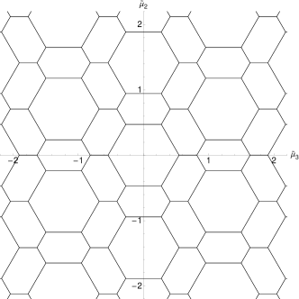
Figure 1: Phase boundaries at zero temperature for $f=3$ in the $\bar{\mu}$ plane (left) and the $\tilde{\mu}$ plane (right).

All $\bar{\mu}$’s inside a given hexagonal cell result in identical $\bar{N}$ as $\tau\to 0$, given by the coordinates of the center of the cell. For example, $\bar{\mu}$’s in the central hexagonal cell lead to $\bar{N}_{2,3}=(0,0)$ at $\tau=0$, the six surrounding cells are characterized by $\bar{N}_{2,3}=\pm(1,\frac{1}{2})$, $\bar{N}_{2,3}=\pm(\frac{1}{2},1)$, and $\bar{N}_{2,3}=\pm(-\frac{1}{2},\frac{1}{2})$. Every vertex is common to three cells. The coordinates of the vertices between the central cell and the six surrounding cells are $\pm(\frac{2}{3},\frac{2}{3})$, $\pm(0,\frac{2}{3})$, $\pm(\frac{2}{3},0)$, $\pm(1,1)$, $\pm(0,1)$, $\pm(1,0)$.

First-order phase transitions occur between neighboring cells with different particle numbers $\bar{N}_{2,3}$ at $\tau=0$. At the edges of the hexagonal cells, two phases can coexist, and at the vertices, three phases can coexist at zero temperature.

In analogy to the two-flavor case, a high-temperature system with small fluctuations (as a function of Euclidean spacetime) of $\bar{\mu}_{2,3}$ can result in two or three phases coexisting or result in a pure state as $\tau\to 0$ depending on the choice of $\bar{\mu}_{2,3}$

3.3 Phase structure for $f=4$

We use Eq. (9) to identify the phase structure in the $(\bar{\mu}_{2},\bar{\mu}_{3},\bar{\mu}_{4})$ space, which is divided into three-dimensional cells characterized by identical particle numbers $\bar{N}_{2,3,4}$ at zero temperature. At the boundaries of these cells, multiple phases can coexist at zero temperature. We find different types of vertices (corners of the cells), where four and six phases can coexist. At all edges, three phases can coexist.

As in the three flavor case, we observe that the phase structure exhibits higher symmetry in coordinates $\tilde{\mu}$ which are related to $\mu$ through an orthonormal transformation. A particularly convenient choice for $f=4$ turns out to be given by

$$\begin{pmatrix}\tilde{\mu}_{1}\\ \tilde{\mu}_{2}\\ \tilde{\mu}_{3}\\ \tilde{\mu}_{4}\end{pmatrix}=\frac{1}{2}\begin{pmatrix}1&1\\ 1&-1\end{pmatrix}\otimes\begin{pmatrix}1&1\\ 1&-1\end{pmatrix}\begin{pmatrix}\mu_{1}\\ \mu_{2}\\ \mu_{3}\\ \mu_{4}\end{pmatrix}$$ (16)

since the phase structure then becomes periodic under shifts parallel to the coordinate axes. The explicit form of an alternative representation of the partition function in these coordinates is given in [7]. At zero temperature the $\tilde{\mu}_{2,3,4}$ space is divided into two types of cells (see Fig. 2 for visualizations). We can think of the first type as a cube (centered at the origin, with side lengths 1 and parallel to the coordinate axes) where all the edges have been cut off symmetrically. The original faces are reduced to smaller squares (perpendicular to the coordinate axes) with corners at $\tilde{\mu}_{2,3,4}=(\pm\frac{1}{2},\pm\frac{1}{4},\pm\frac{1}{4})$ (permutations and sign choices generate the six faces). This determines the coordinates of the remaining 8 corners to be located at $(\pm\frac{3}{8},\pm\frac{3}{8},\pm\frac{3}{8})$. The shift symmetry tells us that these “cubic” cells are stacked together face to face. The remaining space (around the edges of the original cube) is filled by cells of the second type (in the following referred to as “edge” cells), which are identical in shape and are oriented parallel to the three coordinate axes.

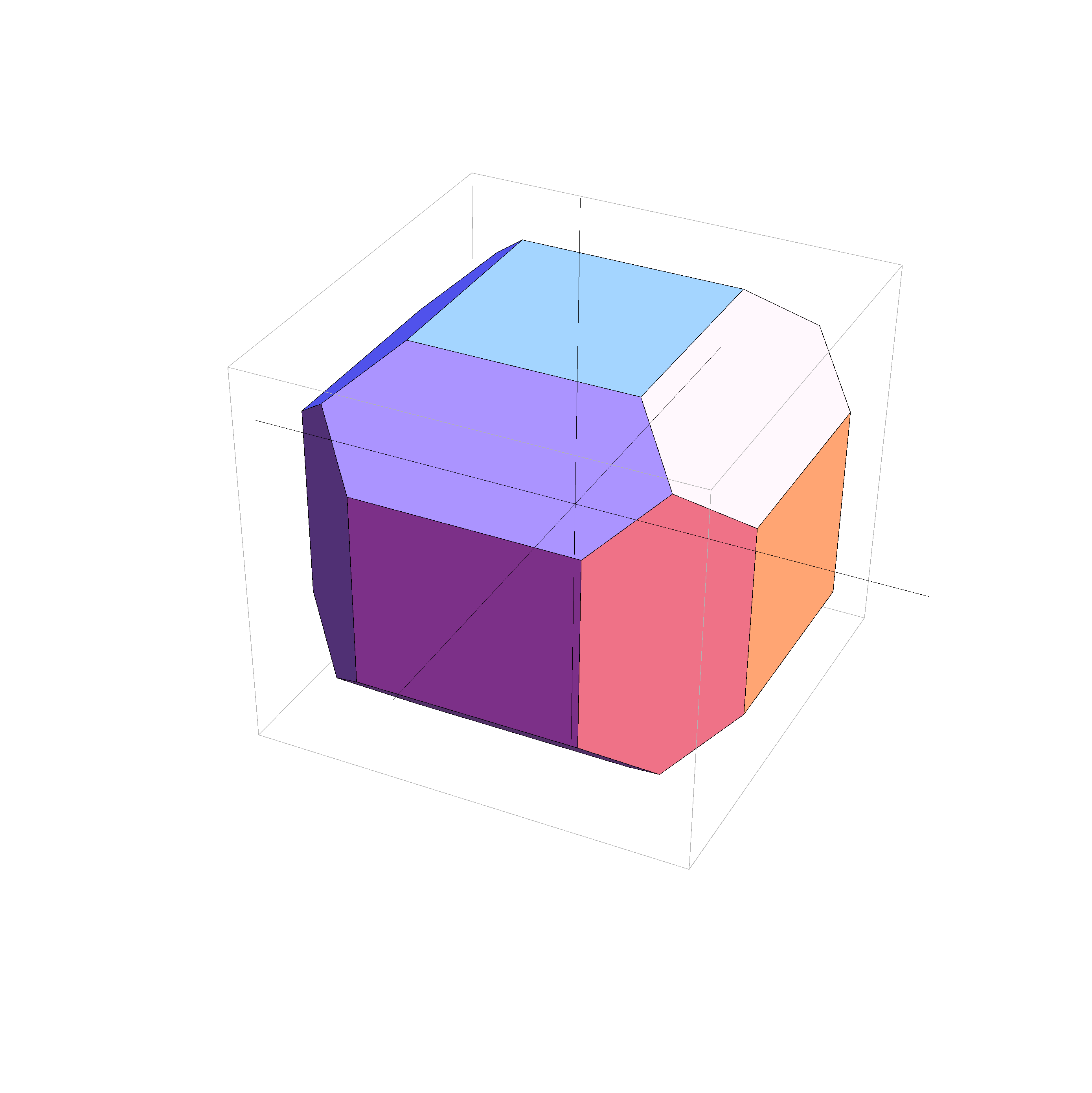
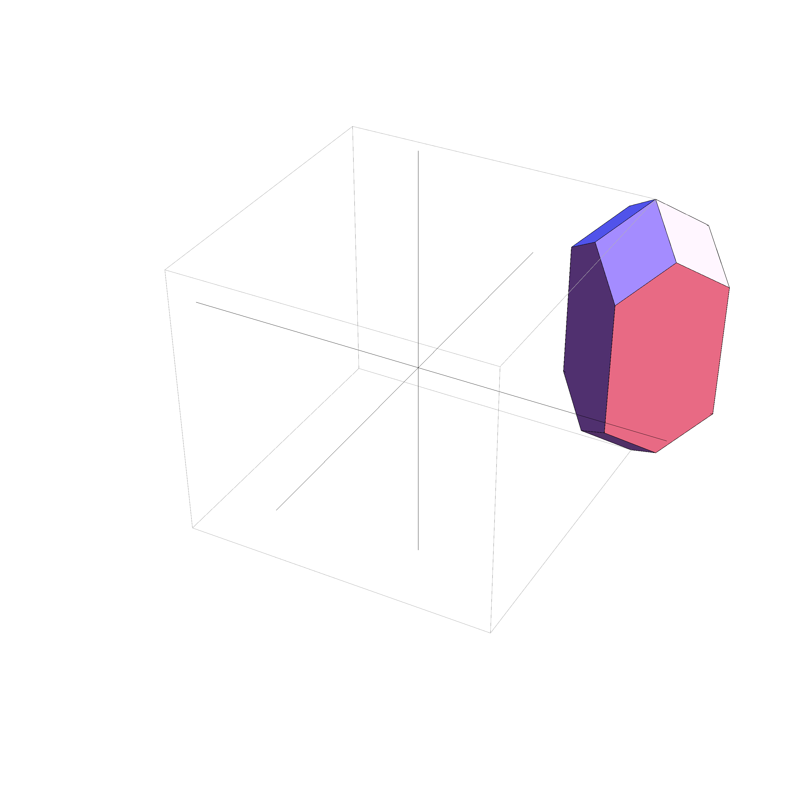
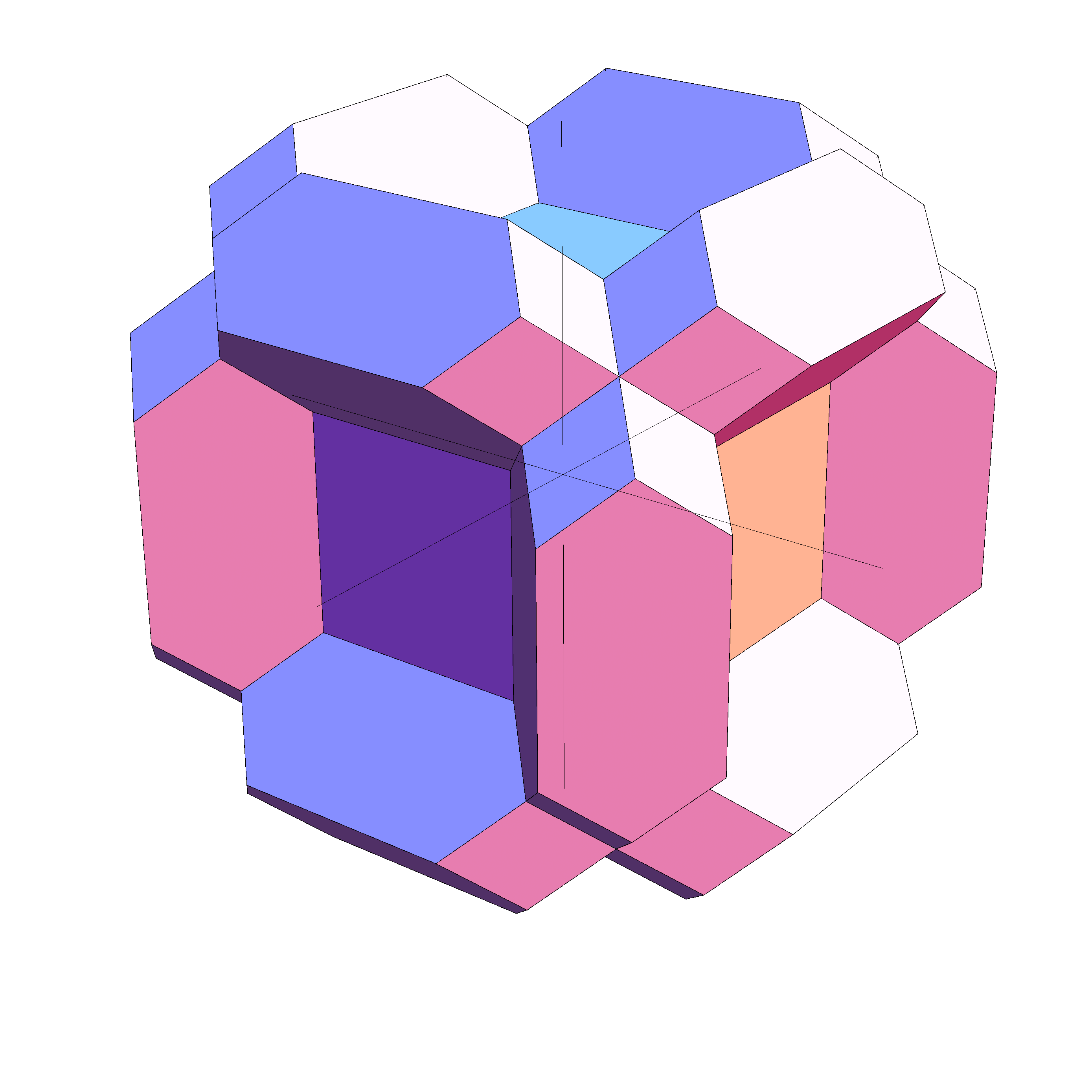
Figure 2: Cells defining the zero-temperature phase structure for $f=4$ in the $\tilde{\mu}$ coordinates as described in the text. The left figure shows the central “cubic” cell, the figure in the center a single “edge” cell. The right figure shows the cubic cell together with all 12 attaching edge cells.

This leads to different kinds of vertices (at the corners of the cells described above) where multiple phases can coexist at zero temperature. There are corners which are common points of two cubic and two edge cells (coexistence of 4 phases, for example at $(\pm\frac{1}{2},\pm\frac{1}{4},\pm\frac{1}{4})$), there are corners which are common points of one cubic and three edge cells (coexistence of 4 phases, for example at $(\pm\frac{3}{8},\pm\frac{3}{8},\pm\frac{3}{8})$), and there are corners which are common points of six edge cells (coexistence of six phases, for example at $\tilde{\mu}_{2,3,4}=(\pm\frac{1}{2},\pm\frac{1}{2},\pm\frac{1}{2})$. Any edge between two of these vertices is common to three cells.

3.4 Phase structure for $f>4$

One can use the multidimensional theta function to study the phase structure when $f>4$ but visualization of the cell structure becomes difficult. Nevertheless, it is possible to provide examples for the coexistence of many phases. While for $f=5$, we find only up to $5\choose 2$ coexisting phases, we find up to $6\choose 3$ coexisting phases for $f=6$ (for example at $\bar{\mu}_{2,\ldots,6}=(1,\frac{1}{2},0,0,0)$). We also find up to $8\choose 4$ coexisting phases for $f=8$ (for example at $\bar{\mu}_{2,\ldots,8}=(1,1,1,1,1,1,0)$). This leads us to conjecture that the maximal number of coexisting phases is given by $f\choose{\lfloor f/2\rfloor}$, increasing exponentially for large $f$.

References

- [1] I. Sachs, A. Wipf and A. Dettki, Phys. Lett. B 317, 545 (1993) [hep-th/9308130].
- [2] I. Sachs and A. Wipf, Annals Phys. 249, 380 (1996) [hep-th/9508142].
- [3] I. Sachs and A. Wipf, Helv. Phys. Acta 65, 652 (1992) [arXiv:1005.1822 [hep-th]].
- [4] D. J. Gross, R. D. Pisarski and L. G. Yaffe, Rev. Mod. Phys. 53, 43 (1981).
- [5] R. Narayanan, Phys. Rev. D 86, 087701 (2012) [arXiv:1206.1489 [hep-lat]].
- [6] R. Narayanan, Phys. Rev. D 86, 125008 (2012) [arXiv:1210.3072 [hep-th]].
- [7] R. Lohmayer and R. Narayanan, arXiv:1307.4969.