Symmetry-protected many-body Aharonov-Bohm effect

Abstract

It is known as a purely quantum effect that a magnetic flux affects the real physics of a particle, such as the energy spectrum, even if the flux does not interfere with the particle’s path - the Aharonov-Bohm effect. Here we examine an Aharonov-Bohm effect on a many-body wavefunction. Specifically, we study this many-body effect on the gapless edge states of a bulk gapped phase protected by a global symmetry (such as $\mathbb{Z}_{N}$) - the symmetry-protected topological (SPT) states. The many-body analogue of spectral shifts, the twisted wavefunction and the twisted boundary realization are identified in this SPT state. An explicit lattice construction of SPT edge states is derived, and a challenge of gauging its non-onsite symmetry is overcome. Agreement is found in the twisted spectrum between a numerical lattice calculation and a conformal field theory prediction.

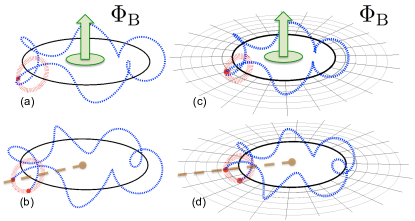
Mysteriously an external magnetic flux can affect the physical properties of particles even without interfering directly on their paths. It is known as the Aharonov-Bohm(AB) effect Aharonov-Bohm. For instance, a particle of charge $q$ and mass $\mathfrak{m}$ confined in a ring (parametrized by $0\leq\theta<2\pi$) of radius $\mathfrak{a}$ threaded with a flux $\Phi_{B}$, see Fig. 1(a), would have its energy spectrum shifted as

$$E_{n}=\frac{1}{2\mathfrak{m}\mathfrak{a}^{2}}\,\left(n+\frac{\Phi_{B}}{\Phi_{0}}\right)^{2},\quad n=0,\pm 1,...,$$ (1)

where $\Phi_{0}=2\pi/q$ is the quantum of magnetic flux and we adopt $e=\hbar=c=1$ units. One can dispose of the gauge potential in the Schrödinger’s equation of the wavefunction $\psi(\theta)$, by a gauge transformation that changes the wavefunction to $\tilde{\psi}(\theta)=\psi(\theta)\,\exp[i\,q\int^{\theta}{\bm{A}}(\theta^{\prime}{})\,d\,\theta^{\prime}]$. So, the effect of the external flux can be enforced by the condition that the phase $\tilde{\varphi}(\theta)$ of the new wavefunction satisfies a twisted boundary condition,

$$(1/2\pi)\,\oint\,d\theta\,\frac{\partial\,\tilde{\varphi}(\theta)}{\partial\theta}=\Phi_{B}/\Phi_{0},$$ (2)

as the particle trajectory encloses the ring; thus, this twisted boundary condition implies a “branch cut”, see Fig. 1(b). We may refer to this twist effect as “Aharonov-Bohm twist”. For electrons confined on a mesoscopic ring, for example, even though interactions are not negligible, the sensitivity of the system to the presence of the external flux can be rationalized as a single particle phenomenon Aronov-Sharvin.

It is then opportune, as matter of principle, to ask whether such an AB effect can take place as an intrinsically interacting many-body phenomenon. More concretely, we ask whether the low energy properties of such interacting systems display a response analogous to Eq. (1) when subject to a gauge perturbation and, in turn, how this effect is encoded in the “topology” (or boundary conditions) of the the wave-functional $\Psi[\phi(x)]$, see Figs. 1(c)-(d). We shall refer to this as a many-body AB effect or twist.

In this paper we show that $2$D “symmetry protected topological”(SPT) states [Chen:2011pg; Chen et al. 2011; Wen:2013ue] offer a natural platform for observing the many-body AB effect. SPT states are quantum many-body states of matter with a finite gap to bulk excitations and no fractionalized degrees of freedom. Due to a global symmetry, the system has the property that its edge states can only be gapped if a symmetry breaking occurs, either explicitly or spontaneously. So, in the absence of any symmetry breaking, the edge is described by robust edge excitations which can not be localized due to weak symmetry-preserving disorder, in contrast to purely one dimensional systems Lee-Ramakrishnan. Assuming then that the edge states are in this gapless phase (an assumption which we will take throughout the paper), we shall demonstrate that the system will respond to the insertion of a gauge flux in a non-trivial way, whereas if the edge degrees of freedom were to become gapped, then they would be insensitive to the flux. We note that in 2D systems displaying the integer quantum Hall effect, the insertion of a flux also induces a non-trivial response of the chiral edge states Laughlin1981. In contrast to this situation, here we shall be concerned with 2D non-chiral SPT states for which the gapless edge excitations, like the single particle modes on a ring, propagate in both directions. The spectrum of these gapless modes characterize the low energy properties of the system.

Figure 1: (a) and (c): Single- and many-body wavefunctions upon flux insertion, respectively. (b) and (d): Flux effect captured by twisted boundary conditions showing the associated branch cut.

We approach this problem from two venues: (I) First we study the response of the SPT state to the insertion of a gauge flux by means of a low energy effective theory for the edge states and derive the change in the spectrum of edge states akin to Eq. (1). (II) Complementarily, we show that the many-body AB effect derived in (I) can also be captured by formulating a lattice model describing the edge states. Twisted boundary conditions defined for these models are shown to account for the presence of a gauge flux, which we confirm numerically.

I Many-body Aharonov-Bohm effect

To capture the essence of AB effect on a symmetry-protected many-body wavefunction, we imagine threading a gauge flux through an effective 1D edge on one side of a $2$D bulk SPT annulus (or cylinder). This many-body wavefunction on the $1$D edge (parametrized by $0\leq x<L$) of SPT states is the analogue of a single-body wavefunction of a particle in a ring. Since the bulk degrees of freedom are gapped, we concentrate on the low energy properties on the edge described by a non-chiral Luttinger liquid action $I_{\textrm{edge}}[\phi_{I}]$ [LevinGu; Lu:2012dt]. To capture the gauge flux effect on a many-body wave function $|\Psi\rangle$, we formulate it in the path integral,

$$\begin{split}&\,|\Psi(t_{f})\rangle=\sum_{n}|\Psi_{n}(t_{f})\rangle\langle\Psi_{n}(t_{f})|e^{-i\int^{t_{f}}_{t_{i}}H(t)dt}|\Psi(t_{i})\rangle\\ &\,=\sum_{n}|\Psi_{n}(t_{f})\rangle\int^{\phi_{I,n}}_{\phi_{I}(t_{i})}\mathcal{D}\phi_{I}e^{i\,(I_{\textrm{edge}}[\phi_{I}]+(1/2\pi)\int q^{I}{\bm{A}}\wedge d\phi_{I})},\end{split}$$ (3)

with $\phi_{I}$ the intrinsic field on the edge. Our goal is to interpret this many-body AB twist $(1/2\pi)\int q^{I}{\bm{A}}\wedge d\phi_{I}$. We anticipate the energy spectrum under the flux would be adjusted, and we aim to capture this “twist” effect on the energy spectrum. Below we focus on bosonic SPT states with $\mathbb{Z}_{N}$ symmetry [LevinGu; Lu:2012dt; Chenggu; Hung:2013nla; Ye:2013upa], with global symmetry transformation on the edge (see Appendix 1 for details on the field theoretic input)

$$\mathcal{S}^{(p)}_{N}=e^{\frac{i}{N}\,\left(\int^{L}_{0}\,dx\,\partial_{x}\phi_{2}+p\,\int^{L}_{0}\,dx\,\partial_{x}\phi_{1}\right)},$$ (4)

where $p\in\{0,...,N-1\}$ and $(1/2\pi)\partial_{x}\phi_{2}(x)$ is the canonical momentum associated to $\phi_{1}(x)$ [Wang:2012am].

The Lagrangian density associated to Eq.(3) reads

$$\mathcal{L}_{\textrm{edge}}[A]=\frac{1}{4\pi}K_{IJ}\,\partial_{t}\phi_{I}\,\partial_{x}\phi_{J}\,-\mathcal{H}_{f}[\phi_{I}]+\frac{1}{2\pi}q^{I}\,A_{\mu}\varepsilon^{\mu\nu}\partial_{\nu}\phi_{I},$$ (5)

where indices $\mu,\nu\in\{0,1\}$, $I,J\in\{1,2\}$, $K=\begin{pmatrix}0&1\\ 1&0\end{pmatrix}$, $\mathcal{H}_{f}[\phi_{I}]$ is the Hamiltonian density describing a free boson and $q^{I}=(q^{1},q^{2})=(1,p)$ specify the charges carried by the currents $J^{\mu}_{I}=(1/2\pi)\varepsilon^{\mu\nu}\partial_{\nu}\phi_{I}$. The right/left moving modes are described by $\phi_{R,L}\propto\phi_{1}\pm\phi_{2}$.

Integrating the equations of motion of (5), with respect to $\phi_{I}$, along the boundary coordinate $x$ in the presence of a static background $\mathbb{Z}_{N}$ gauge flux configuration $\oint^{L}_{0}dxA_{1}(x)=\frac{2\pi}{N}$ delivers

$$\begin{split}&\,(1/2\pi)\oint^{L}_{0}dx\,\partial_{x}\begin{pmatrix}\phi_{1}\\ \phi_{2}\end{pmatrix}=\frac{1}{N}\begin{pmatrix}p\\ 1\end{pmatrix}.\end{split}$$ (6)

(See Appendix 2 for an alternative derivation from a bulk-edge Chern-Simons approach). Eq. (6) represents the shift in winding modes of the edge boson fields and plays a role analogous to the single-particle twisted boundary condition Eq. (2). The spectrum of the central charge $c=1$ free boson at compactification radius $R$ is labeled by the primary states $|n,m\rangle$ ($n,m\in\mathbb{Z}$) with scaling dimension

$$\Delta(n,m;R)=\frac{n^{2}}{R^{2}}+\frac{R^{2}m^{2}}{4}$$ (7)

and momentum $\mathcal{P}(n,m)=nm$ DiFrancesco. Then, according to Eq. (6), after the flux insertion, we derive the new spectrum (also see another related setting Sule:2013qla)

$$\begin{split}&\,\tilde{\Delta}^{(p)}_{N}(n,m;R)=\frac{1}{R^{2}}\left(n+\frac{p}{N}\right)^{2}+\frac{R^{2}}{4}\left(m+\frac{1}{N}\right)^{2}\end{split}$$ (8)

and momenta $\tilde{\mathcal{P}}^{(p)}_{N}(n,m)=\left(n+\frac{p}{N}\right)\left(m+\frac{1}{N}\right)$ for each SPT state $p\in\{0,...,N-1\}$. Eqs. (6) and (8) capture the essence of the many-body AB effect analogous to Eqs. (1) and (2).

II Effective lattice model for the edge of SPT states

-Symmetry transformation and domain wall-
The twist effect encoded in Eq. (8) comes from an effective low energy description of the edge. We aim, as a complementary and perhaps more fundamental point of view, to capture this twist effect from a lattice model. As a first step in this program, we shall construct a global $\mathbb{Z}_{N}$ symmetry transformation in terms of discrete degrees of freedom on the edge whose action reduces to Eq. (4) at long wavelengths. The hallmark of a non-trivial SPT state is that the symmetry transformation on the boundary cannot be in a tensor product form on each single site, i.e., it acts as a non-onsite symmetry transformation [Chen:2011pg; Chen et al. 2011; Chen:2012hc]. We propose the following ansatz for the symmetry transformation,

$$\begin{split}\bullet\;\;\;S^{(p)}_{N}&\,\equiv\prod^{M}_{j=1}\tau_{j}\prod^{M}_{j=1}\exp\Big\{i\frac{p}{N}\big[\frac{2\pi}{N}(\delta N_{\text{DW}})_{j,j+1}\big]\Big\}\\ &\,\equiv\prod^{M}_{j=1}\tau_{j}\;\prod^{M}_{j=1}e^{\frac{i}{N}\,Q^{(p)}_{N}(\sigma^{\dagger}_{j}\sigma_{j+1})},\end{split}$$ (9)

acting on a ring with $M$ sites that we take to describe the $1$D edge, with $\sigma_{M+1}\equiv\sigma_{1}$. At every site of the ring we consider a pair of two $\mathbb{Z}_{N}$ operators: $(\tau_{j},\sigma_{j})$, with a site index $j=1,...,M$, satisfying $\tau^{N}_{j}=\sigma^{N}_{j}=\openone$ and a conjugation relation $\tau^{\dagger}_{j}\,\sigma_{j}\,\tau_{j}=\omega\,\sigma_{j}$, where $\omega\equiv e^{i\,2\pi/N}$. We shall use the following representation

$$\begin{split}&\,\sigma_{j}={\begin{pmatrix}1&0&0&0\\ 0&\omega&0&0\\ 0&0&\ddots&0\\ 0&0&0&\omega^{N-1}\end{pmatrix}}_{j}\,,\\ &\,\tau_{j}={\begin{pmatrix}0&0&0&\dots&0&1\\ 1&0&0&\dots&0&0\\ 0&1&0&\dots&0&0\\ 0&0&1&\dots&0&0\\ \vdots&0&0&\dots&1&0\end{pmatrix}}_{j}\,.\end{split}$$ (10)

The operators act on the Hilbert space of $\mathbb{Z}_{N}$ states for each site $j$.

The overall symmetry transformation contains the onsite transformation part generated by the string of $\tau$’s and the “non-onsite domain wall (DW)” part $(\delta N_{\text{DW}})_{j,j+1}$ between sites $j$ and $(j+1)$. The ansatz form Eq. (9) has the property that $\prod^{M}_{j=1}\tau_{j}$ and $\prod^{M}_{j=1}e^{\frac{i}{N}\,Q^{(p)}_{N}(\sigma^{\dagger}_{j}\sigma_{j+1})}$ commute, and the unitarity of $S^{(p)}_{N}$ implies $[Q^{(p)}_{N}]^{\dagger}=Q^{(p)}_{N}$. It follows that

$$\Big(\,S^{(p)}_{N}\,\Big)^{N}=\prod^{M}_{j=1}\,e^{i\,Q^{(p)}_{N}(\sigma^{\dagger}_{j}\sigma_{j+1})}\,.$$ (11)

•The construction above then naturally yields $N$ distinct classes of $\mathbb{Z}_{N}$ symmetry transformations, labeled by $p\in\mathbb{Z}_{N}$, upon imposing the following condition on the $(N-1)$-th order polynomial operator $Q^{(p)}_{N}(\sigma^{\dagger}_{j}\sigma_{j+1})$:

$$e^{i\,Q^{(p)}_{N}(\sigma^{\dagger}_{j}\sigma_{j+1})}=(\sigma^{\dagger}_{j}\sigma_{j+1})^{p},\quad p=0,...,N-1,$$ (12)

which guarantees (due to periodic boundary conditions) that $(S^{(p)}_{N})^{N}=\openone$. The symmetry transformation in the trivial case corresponds to $p=0\,(\text{mod}\,N)$ for which $\prod_{j}e^{\frac{i}{N}\,Q^{(p=0)}_{N}(\sigma^{\dagger}_{j}\sigma_{j+1})}=\openone$, while $p\neq 0\,(\text{mod}\,N)$ describe the other $N-1$ non-trivial SPT classes. Identifying $\sigma_{j}\sim e^{i\,\phi_{1}(j)}$, then the domain wall variable $(\delta N_{\text{DW}})_{j,j+1}$ counts the number of units of $\mathbb{Z}_{N}$ angle between sites $j$ and $j+1$, so $(2\pi/N)(\delta N_{\text{DW}})_{j,j+1}$$=\phi_{1,j+1}-\phi_{1,j}$, which produces the expected long distance behavior of the symmetry transformation Eq. (4). Our ansatz nicely embodies two interpretations together, on both a continuum field theory and a discrete lattice model. The $\mathbb{Z}_{N}$ symmetry transformations Eq. (9) that satisfy Eq. (12) can be explicitly written as

$$S^{(p)}_{N}=\prod^{M}_{j=1}\tau_{j}\,\prod^{M}_{j=1}e^{-i\frac{2\pi}{N^{2}}p\,\Big\{\left(\frac{N-1}{2}\,\right)\openone+\sum^{N-1}_{k=1}\,\frac{(\sigma^{\dagger}_{j}\sigma_{j+1})^{k}}{(\omega^{k}-1)}\Big\}}.$$ (13)

•In Ref.Chen:2012hc the edge symmetry for $\mathbb{Z}_{N}$ SPT states was proposed in terms of effective long-wavelength rotor variables. We emphasize that the construction of the edge symmetry transformations Eq. (13) described here does not rely on a long wavelength description; rather it can be viewed as a fully regularized symmetry transformation. In Appendices 3 and 4, we give explicit formulas for the $\mathbb{Z}_{2}$ and $\mathbb{Z}_{3}$ symmetry transformations, as well as we draw a connection between the lattice operators $(\tau_{j},\sigma_{j})$ and quantum rotor variables.

-Lattice model-
Having constructed all the classes of $\mathbb{Z}_{N}$ symmetry transformations Eq. (13), we now propose our translation invariant and $\mathbb{Z}_{N}$-symmetric lattice model Hamiltonians $H^{(p)}_{N}$ on the edge of $\mathbb{Z}_{N}$ SPT states, i.e.,

$$[H^{(p)}_{N},T]=0,\;\;[H^{(p)}_{N},S^{(p)}_{N}]=0,$$ (14)

where $T$ performs a translation by one lattice site. Our model Hamiltonian is (with $\lambda^{(p)}_{N}$ a constant),

$$H^{(p)}_{N}\!\!=\!\lambda^{(p)}_{N}\!\sum^{M}_{j=1}\!h^{(p)}_{N,j}\!\equiv\!-\lambda^{(p)}_{N}\!\sum^{M}_{j=1}\!\!\sum^{N-1}_{\ell=0}\!\!\left(S^{(p)}_{N}\right)^{\!\!-\ell}\!\!\!(\tau_{j}+\tau^{\dagger}_{j})\!\!\left(S^{(p)}_{N}\right)^{\ell}.$$ (15)

Notice that $H^{(p)}_{N}$ is manifestly $\mathbb{Z}_{N}$ symmetric since it is constructed from the superposition of $\tau_{j}$ conjugated to all powers of $S^{(p)}_{N}$. In the trivial SPT case for which $H^{(p=0)}_{N}\propto-\sum^{M}_{j=1}\,(\tau_{j}+\tau^{\dagger}_{j})$, the model gives a gapped and symmetry preserving ground state. In Appendix 3, we provide explicit forms of the non-trivial classes of SPT Hamiltonians for the $N=2$ and $N=3$ cases. We note that for the $\mathbb{Z}_{2}$ case, our symmetry transformation and edge Hamiltonian are the same as that obtained in Ref. LevinGu (where the low energy theory in terms of a non-chiral Luttinger liquid has been discussed), despite the fact that our method of constructing the symmetry is independent of that in Ref. LevinGu and provides a generalization for all $\mathbb{Z}_{N}$ groups. It is noteworthy to mention that the authors of Ref. LevinGu argue that the edge of the $\mathbb{Z}_{2}$ bosonic SPT state is generically unstable to symmetry preserving perturbations. Nevertheless, we shall still study the model Hamiltonian (15) for the $\mathbb{Z}_{2}$ as a means to address our numerical methods. A common feature of these Hamiltonian classes is the existence of combinations of terms like $\sigma_{j-1}\tau_{j}\sigma_{j+1}$ due to the non-onsite global symmetry. Their effect, as we shall see, is to give rise to a gapless spectrum. In order to understand their effect on the low energy properties, we perform an exact diagonalization study of the non-trivial Hamiltonian classes Eq. (15) on finite systems.

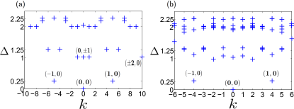
In Fig. (2) we plot the lowest energy eigenvalues for the $\mathbb{Z}_{2}$ and $\mathbb{Z}_{3}$ non-trivial SPT states as a function of the lattice momentum $k\in\mathbb{Z}$ defined by $T=e^{i\frac{2\pi}{M}k}$. The spectrum of $H^{(1)}_{2}$ with $M=20$ sites, shows very good agreement with the bosonic spectrum Eq. (7) at $R=2$, with states being labeled by $|n,m\rangle$. The global $\mathbb{Z}_{2}$ charges relative to the ground state were found to be $e^{i\,\pi\,(n+m)}$ in accordance to Eq. (4) (We note that similar results have been obtained for the $\mathbb{Z}_{2}$ case in Ref. Chen:2012hc). For the $\mathbb{Z}_{3}$ SPT states, which have not been investigated before, with $M=12$ sites, the spectrum of $H^{(1)}_{3}$ and $H^{(2)}_{3}$ are identical H. Finite size effects are more prominent than in the $\mathbb{Z}_{2}$ case, but the overall structure of the spectrum is very similar with the second and third states being degenerate with energy close to $1/4$ and global $\mathbb{Z}_{3}$ charges $e^{\pm 2\pi i/3}$ (which we identify as the $|n=\pm 1,m=0\rangle$ states), suggesting the same spectrum Eq. (7) at $R=2$.

Figure 2: Spectrum of the SPT Hamiltonian Eq. (15) with respect to the lowest energy $E^{(p)}_{N,0}$, on a ring as a function of the lattice momentum $k\in\mathbb{Z}$. First few primary states labeled by $(n,m)$. (a) Spectrum of $H^{(p=1)}_{2}$ with $\lambda^{(p=1)}_{2}=0.82$ and $M=20$ sites. (b) Spectrum of $H^{(p=1,2)}_{3}$ with $\lambda^{(p=1,2)}_{3}=0.26$ and $M=12$ sites. The values of $\lambda^{(p)}_{N}$ above guarantee a proper normalization so that states in the same conformal tower separated by $\delta k=\pm 1$ are integer spaced (up to finite size effects) [see Ref. Henkel].

In Appendix 4, following the methods of Refs. [Chen:2012hc; Chen et al. 2011; Chen:2011pg], we show that the symmetry classes defined in Eq. (9) subject to condition Eq. (12) are related to all $\mathbb{Z}_{N}$ $3$-cocycles of the group cohomology classification of $2$D SPT states [Chen:2011pg]. Thus, our lattice model completely realizes all $N$ classes of $\mathcal{H}^{3}(\mathbb{Z}_{N},U(1))=\mathbb{Z}_{N}$, where $p$ stands for the $p$-th class in the third cohomology group.

III Twisted boundary conditions and Twisted Hamiltonian on the lattice

We now seek to build a lattice model with twisted boundary conditions to capture the edge states spectral shift in the presence of a unit of $\mathbb{Z}_{N}$ flux insertion.

It is instructive to revisit the case of twisted boundary conditions where the symmetry transformation acts as an on-site symmetry. For the sake of concreteness, let us consider the one dimensional quantum Ising model $H_{Ising}=\sum^{M}_{j=1}\,(J\,\sigma^{z}_{j}\,\sigma^{z}_{j+1}+h\,\sigma^{x}_{j})$ with global $\mathbb{Z}_{2}$ symmetry $\prod^{M}_{j=1}\,\sigma^{x}_{j}$. The $\mathbb{Z}_{2}$ twisted sector (or equivalently, in this case, the anti-periodic boundary condition sector) of the model is realized by flipping the sign of a pair interaction $\sigma^{z}_{k}\sigma^{z}_{k+1}\rightarrow-\sigma^{z}_{k}\sigma^{z}_{k+1}$, for some site $k$, while leaving all the other terms unchanged. If the Ising model is defined on an open line, the twist effect is implemented by conjugating the $H_{Ising}$ with the operator $\prod_{\ell\leq k}\,\sigma^{x}_{\ell}.$ When the model is defined on a ring, the same effect is obtained by defining a new translation operator $\tilde{T}=T\,\sigma^{x}_{k}$ and demanding that the twisted Hamiltonian $\tilde{H}_{Ising}$ commutes with $\tilde{T}$. It is straightforward to see that the twisted Ising Hamiltonian on a ring which commutes with $\tilde{T}$ indeed has $\sigma^{z}_{k}\sigma^{z}_{k+1}\rightarrow-\sigma^{z}_{k}\sigma^{z}_{k+1}$. We also note that $(\tilde{T})^{M}=\prod^{M}_{j=1}\,\sigma^{x}_{j}$ generates the $\mathbb{Z}_{2}$ symmetry of $H_{Ising}$, which is also a symmetry of $\tilde{H}_{Ising}$.

We now generalize the construction above for the SPT edge Hamiltonians on a ring with a non-onsite symmetry by defining the unitary twisted lattice translation operatormany-flux-case

$$\tilde{T}^{(p)}=T\,e^{\frac{i}{N}\,Q^{(p)}_{N}(\sigma^{\dagger}_{M}\sigma_{1})}\tau_{1},$$ (16)

for each $p\in\mathbb{Z}_{N}$ classes, which incorporates the effect of the branch cut as in Fig. 1(d). The twisted Hamiltonian $\tilde{H}^{(p)}_{N}$, constructed from ${H}^{(p)}_{N}$ of Eq. (15) and satisfying

$$[\tilde{H}^{(p)}_{N},\tilde{T}^{(p)}]=0,\;\;\;$$ (17)

reads (see Appendix 3.2 for explicit results)

$$\tilde{H}^{(p)}_{N}=\lambda^{(p)}_{N}\sum^{M}_{j=1}\tilde{h}^{(p)}_{N,j}$$ (18a)

•

$$\begin{split}&\,\tilde{h}^{(p)}_{N,1}=\tau^{\dagger}_{1}\,\tau^{\dagger}_{2}\,h^{(p)}_{N,1}\tau_{1}\,\tau_{2},\\ &\,\tilde{h}^{(p)}_{N,j}=h^{(p)}_{N,j}~(2\leq j\leq M-1),\\ &\,\tilde{h}^{(p)}_{N,M}=\tau^{\dagger}_{1}\,e^{-\frac{i}{N}\,Q^{(p)}_{N}(\sigma^{\dagger}_{M}\sigma_{1})}\,h^{(p)}_{N,M}\,e^{\frac{i}{N}\,Q^{(p)}_{N}(\sigma^{\dagger}_{M}\sigma_{1})}\tau_{1}.\end{split}$$ (18b)

•

Notice that, due to the intrinsic non-onsite term in the symmetry transformation,

$$\tilde{S}^{(p)}_{N}\equiv(\tilde{T}^{(p)})^{M}=e^{\frac{i}{N}\Big[Q^{(p)}_{N}(\omega\,\sigma^{\dagger}_{M}\,\sigma_{1})-Q^{(p)}_{N}(\sigma^{\dagger}_{M}\,\sigma_{1})\Big]}\,S^{(p)}_{N}\,,$$ (19)

the twisted non-trivial Hamiltonian breaks the SPT global symmetry (i.e. $[\tilde{H}^{(p)}_{N},S^{(p)}_{N}]\neq 0$ if $p\neq 0$ mod($N$) ), signaling an anomaly effectWen:2013oza; Wang:2014tia. (For a more systematic discussion of bosonic anomalies in the context of $2$D SPT states, see Ref.[Wang:2014tia].) However, in the trivial state, Eq. (19) yields $\tilde{S}^{(p=0)}_{N}=S^{(p=0)}_{N}=\prod^{M}_{j=1}\tau_{j}$, so that the twisted trivial Hamiltonian still commutes with the global $\mathbb{Z}_{N}$ onsite symmetry, and the twisted effect is equivalent to usual toroidal boundary conditions Henkel, as exemplified before for anti-periodic boundary condition of the Ising model.

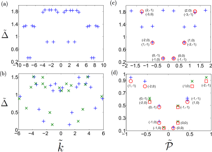
In Figs. (3 a) and (3 b) we display the low energy spectrum of the twisted $\mathbb{Z}_{2}$ and $\mathbb{Z}_{3}$ SPT Hamiltonians with a $\pi$-flux and $2\pi/3$-flux, respectively, as a function of twisted lattice momentum $\tilde{k}$ defined as $\tilde{T}=e^{i\,\frac{2\pi}{M}\tilde{k}}$. The eigenvalues of the primary states show very good agreement with $\tilde{\Delta}^{(1)}_{2}(n,m;R=2)$ and $\tilde{\Delta}^{(1,2)}_{3}(n,m;R=2)$ in Eq. (8), which we compare, in Figs. (3 c) and (3 d), by folding the spectrum so that the primary states are plotted as a function of the continuum momenta $\tilde{\mathcal{P}}^{(1)}_{2}(n,m)$ and $\tilde{\mathcal{P}}^{(1,2)}_{3}(n,m)$. Our findings thus establish a relationship between the many-body AB effect both in terms of a long wavelength description in the field theory as well as in terms of twisted boundary conditions in a lattice model.

Figure 3: Spectrum of the twisted SPT Hamiltonian with respect to the lowest energy $E^{(p)}_{N,0}$ on a ring as a function of the lattice momentum $\tilde{k}$, with the same values of $\lambda^{(p)}_{N}$ as in Fig. (2). First few primary states labeled by $(n,m)$. (a) Spectrum of $\tilde{H}^{(1)}_{2}$ with $M=20$ sites. (b) Spectrum of $\tilde{H}^{(1)}_{3}$ (+) and $\tilde{H}^{(2)}_{3}$ ($\times$) with $M=12$ sites. (c) Comparison between $\tilde{\Delta}^{(1)}_{2}$ (circles) and numerical results (+) plotted as a function of the momentum $\tilde{\mathcal{P}}^{(1)}_{2}$. All points are two-fold degenerate. Red circles represent primary states, while the remaining points account for descendant states in the CFT spectrum. (d) Comparison between $\tilde{\Delta}^{(1)}_{3}$ (circles) and data points (+) plotted in terms of the momentum $\tilde{\mathcal{P}}^{(1)}_{3}$. Same for $\tilde{\Delta}^{(2)}_{3}$ (squares) and data points ($\times$) plotted in terms of the momentum $\tilde{\mathcal{P}}^{(2)}_{3}$.

IV Summary

We have demonstrated that an intrinsically many-body realization of the Aharonov-Bohm phenomenon takes place on the edge of a $2$D symmetry-protected many-body system in the presence of a background gauge flux. In our construction we have assumed that edge state is in a gapless phase and is described by a simple non-chiral Luttinger liquid action with one right and one left moving propagating modes carrying different $\mathbb{Z}_{N}$ charges Comment, in which case, the spectrum in the presence of a gauge flux displays quantization as Eq.(8) due to global symmetry protection ($\mathbb{Z}_{N}$ symmetry in our work), analogous to the quantization of the energy spectrum of a superconducting ring due to the $\mathbb{Z}_{2}$ symmetry inherent to superconductorsByers:1961zz. The universal information carried by the counter propagating edge modes is that they carry different $\mathbb{Z}_{N}$ charges, which has been numerically verified for the $\mathbb{Z}_{2}$ and $\mathbb{Z}_{3}$ SPT classes in Fig. (2), where this difference is parametrized by the integer $p\in\{1,...,N-1\}$ that characterizes the SPT class. This quantum number should remain invariant as long as the SPT order is not destroyed in the bulk. The offset in the charges carried by the right and left moving modes has then been shown to reflect itself in the edge spectrum according to Eq. (8) (where $R$ is a non-universal parameter), which we have confirmed numerically in our model Hamiltonians for the $\mathbb{Z}_{2}$ and $\mathbb{Z}_{3}$ SPT classes in Fig. (3).

We have proposed general principles guiding the construction of the lattice Hamiltonians, Eqs. (15) and (18b), of the bosonic $\mathbb{Z}_{N}$-symmetric SPT edge states for both the untwisted/twisted (without/with gauge fluxes) cases.

The twisted spectra (i.e. with gauge flux) characterize all types of $\mathbb{Z}_{N}$ bosonic anomaliesWen:2013oza; Wang:2014tia, which naturally serve as “SPT invariantsWen:2013ue” to detect and distinguish all $\mathbb{Z}_{N}$ classes of SPT states numerically/experimentally. (See also recent worksZaletel; Wang:2014tia.)

Gauging a non-onsite symmetry of SPT has been noticed relating to Ginsparg-Wilson(G-W) fermionGinsparg:1981bj approach of a lattice field theory problemWang:2013yta. We remark that our current work achieves gauging a non-onsite symmetry for a bosonic system, thus providing an important step towards this direction. Whether our work can be extended to more general symmetry classes and to fermionic systems (such as U(1) symmetry in G-W fermion approach) is an open question, which we leave for future works.

Appendix

In Appendix 1, we briefly review the field theory tool for topological states, especially symmetry-protected topological (SPT) states, but with the emphasis on the canonical quantization, and how the global symmetry transformation $\mathcal{S}^{(p)}_{N}$ on the edge is encoded in the canonical quantization. Using the same formalism, in Appendix 2, we derive the twisted boundary condition due to a gauge flux insertion.

In Appendix 3, we provide our detailed lattice construction (with $\mathbb{Z}_{N}$ symmetry) for both the untwisted/twisted (without/with gauge flux) cases.

In Appendix 4, we match each SPT class of our lattice construction to the 3-cocycles in the group cohomology classification.

Appendix A 1. Field Theory Realization of $\mathbb{Z}_{N}$ SPT States

A.1 1.1. Bulk and boundary actions

A general framework of categorizing and classifying Abelian topological orders, especially the SPT ones, in 2+1D, makes use of Abelian $K$-matrix Chern-Simons theoryWenbook. We now derive the $K$-matrix construction for the SPT order, following the pioneering worksLevinGu; Lu:2012dt; Chenggu; Wang:2012am; Hung:2013nla; Ye:2013upa.

The intrinsic field theory description of SPT states, on a 2D spatial surface $\mathcal{M}^{2}$, is the Chern-Simons action

$$I_{SPT,\mathcal{M}^{2}}=\frac{1}{4\pi}\int dt\;d^{2}xK_{IJ}\epsilon^{\mu\nu\rho}a^{I}_{\mu}\partial_{\nu}a^{J}_{\rho}\;$$ (20)

where $a$ is the intrinsic(or statistical) gauge field, and $K$ is the $K$-matrix which categorizes the SPT orders. An SPT state is not intrinsically topologically orderedChen:2011pg, so it has no topological degeneracyWenbook; Wang:2012am. Ground state degeneracy(GSD) of SPT on the torus is $\mathop{\mathrm{GSD}}=|\det K|=1$Wenbook; Lu:2012dt; Wang:2012am, this suggests a constrained canonical form of $K$Lu:2012dt; Wang:2012am; Ye:2013upa.

The SPT order is symmetry-protected, so tautologically its order is protected by a global symmetry. The novel features of SPT distinct from a trivial insulator is its symmetry-protected edge states on the boundary. The effective degree of freedom of its 1D edge, $\partial\mathcal{M}^{2}$, is chiral bosonic field $\phi$, where $\phi$ is meant to preserve gauge invariance on the bulk-edge under gauge transformation of the field $a$Wenbook. The boundary action shows

$$I_{SPT,\partial\mathcal{M}^{2}}=\frac{1}{4\pi}\int dt\;dx\;\big(K_{IJ}\partial_{t}\phi_{I}\partial_{x}\phi_{J}-V_{IJ}\partial_{x}\phi_{I}\partial_{x}\phi_{J}\big).$$ (21)

A.2 1.2 $\mathbb{Z}_{N}$ symmetry transformation

The $\mathbb{Z}_{N}$ symmetry simply requires a rank-2 $K$-matrix, which exhausts all the group cohomology class, $\mathcal{H}^{3}(\mathbb{Z}_{N},U(1))=\mathbb{Z}_{N}$,

$$K=\bigl({\begin{smallmatrix}0&1\\ 1&0\end{smallmatrix}}\bigl).$$ (22)

The $\mathbb{Z}_{N}$ symmetry transformation with a $\mathbb{Z}_{N}$ angle specifies the group element $g$Lu:2012dt,

$$g_{n}:\delta\phi_{g_{n}}=\frac{2\pi}{N}n{\begin{pmatrix}1\\ p\end{pmatrix}},\;$$ (23)

where $p$ labels the $\mathbb{Z}_{N}$ class of the cohomology group $\mathcal{H}^{3}(\mathbb{Z}_{N},U(1))=\mathbb{Z}_{N}$. Both $n$ and $p$ are module $N$ as elements in $\mathbb{Z}_{N}$. It can be shown that under $\phi_{g_{n}}\to\phi_{g_{n}}+\delta\phi_{g_{n}}$, the action Eq. (21) is invariant, and the $\mathbb{Z}_{N}$ group structure is realized through $g_{n}^{N}=\openone$. The construction of more general symmetry classes can be found in Ref.Lu:2012dt; Ye:2013upa.

A.3 1.3 Canonical quantization

Here we go through the canonical quantization of the boson field $\phi_{I}$. For canonical quantization, we mean that imposing a commutation relation between $\phi_{I}$ and its conjugate momentum field $\Pi_{I}(x)=\frac{\delta{L}}{\delta(\partial_{t}\phi_{I})}=\frac{1}{2\pi}K_{IJ}\partial_{x}\phi_{J}$. Because $\phi_{I}$ is a compact phase of a matter field, its bosonization contains both zero mode ${\phi_{0}}_{I}$ and winding momentum $P_{\phi_{J}}$, in addition to non-zero modesWang:2012am:

$$\phi_{I}(x)={\phi_{0}}_{I}+K^{-1}_{IJ}P_{\phi_{J}}\frac{2\pi}{L}x+i\sum_{n\neq 0}\frac{1}{n}\alpha_{I,n}e^{-inx\frac{2\pi}{L}}.$$ (24)

The periodic boundary has size $0\leq x<L$. Firstly we impose the commutation relation for zero mode and winding modes, and generalized Kac-Moody algebra for non-zero modes:

$$[{\phi_{0}}_{I},P_{\phi_{J}}]=i\delta_{IJ},\;\;[\alpha_{I,n},\alpha_{J,m}]=nK^{-1}_{IJ}\delta_{n,-m}.$$ (25)

We thus derive canonical quantized fields with the commutation relation:

$$[\phi_{I}(x_{1}),K_{I^{\prime}J}\partial_{x}\phi_{J}(x_{2})] = {2\pi}i\delta_{II^{\prime}}\delta(x_{1}-x_{2}),$$ (26)

$$\;\;[\phi_{I}(x_{1}),\Pi_{J}(x_{2})] = i\delta_{IJ}\delta(x_{1}-x_{2}).$$ (27)

The symmetry transformation of Eq. (23) imples $\phi_{g_{n}}\to\phi_{g_{n}}+\delta\phi_{g_{n}}$:

$${\begin{pmatrix}\phi_{1}(x)\\ \phi_{2}(x)\end{pmatrix}}\to{\begin{pmatrix}\phi_{1}(x)\\ \phi_{2}(x)\end{pmatrix}}+\frac{2\pi}{N}{\begin{pmatrix}1\\ p\end{pmatrix}}.$$ (28)

It can be easily checked, using Eq. (26), that

$$\mathcal{S}^{(p)}_{N}=e^{\frac{i}{N}\,\left(\int^{L}_{0}\,dx\,\partial_{x}\phi_{2}+p\,\int^{L}_{0}\,dx\,\partial_{x}\phi_{1}\right)}$$ (29)

implements the global symmetry transformation

$$\mathcal{S}^{(p)}_{N}{\begin{pmatrix}\phi_{1}(x)\\ \phi_{2}(x)\end{pmatrix}}(\mathcal{S}^{(p)}_{N})^{-1}={\begin{pmatrix}\phi_{1}(x)\\ \phi_{2}(x)\end{pmatrix}}+\frac{2\pi}{N}{\begin{pmatrix}1\\ p\end{pmatrix}}.$$ (30)

Appendix B 2. Twisted boundary condition from a gauge flux insertion

Here we apply the canonical quantization method to formulate the effect of a gauge flux insertion through a cylinder (an analog of Laughlin thought experiments Laughlin1981) in terms of a twisted boundary condition effect. The canonical quantization approach here can be compared with the alternate path integral approach motivated in the main text. The canonical quantization offers a solid view why the twisted boundary condition resulted from a gauge flux is a quantum effect. We will firstly present the bulk theory viewpoint, then the edge theory viewpoint.

B.1 2.1 Bulk theory

Our setting is an external adiabatic gauge flux insertion through a cylinder/annulus. Here the gauge field (such as electromagnetic field) couples to (SPT or intrinsic) topologically ordered states, by a coupling charge vector $q_{I}$. The bulk term (here we recover the right dimension, while one can set these to be $e=\hbar=c=1$ in the end)

$$I_{bulk}=\int_{\mathcal{M}}(c\;dt)\;d^{2}x\;\Big((\frac{e^{2}}{\hbar})\;\frac{K_{IJ}}{4\pi}\epsilon^{\mu\nu\rho}a^{I}_{\mu}\partial_{\nu}a^{J}_{\rho}+eq^{I}A_{\mu}J^{\mu}_{I}\Big),$$ (31)

where $J^{\mu}_{I}$ is in a conserved current form

$$J^{\mu}_{I}=(\frac{e}{\hbar})\frac{1}{2\pi}\epsilon^{\mu\nu\rho}\partial_{\nu}a_{\rho,I}.$$ (32)

From the action, we derive the EOM

$$J_{J}^{\mu}=-q_{I}\frac{e}{2\pi}K^{-1}_{IJ}\frac{c}{\hbar}\epsilon^{\mu\nu\rho}\partial_{\nu}A_{\rho}.$$ (33)

From the bulk theory side, an adiabatic flux $\Delta\Phi_{B}$ induces an electric field ${E}_{x}$ by Faraday effect, causing a perpendicular current $J_{y}$ flow to the boundary edge states. We can explicitly derive the flux effect from Faraday-Maxwell equation in the 2+1D bulk,

$$q_{I}\Delta\Phi_{B} = -q_{I}\int dt\int\vec{E}\cdot d\vec{l}=q_{I}\int dt\;dl_{\mu}\;c\;\epsilon^{\mu\nu\rho}\partial_{\nu}A_{\rho}$$ (34)

$$= -\frac{2\pi}{e}K_{IJ}\hbar\int J_{y,J}dtdx=-\frac{2\pi}{e}K_{IJ}\frac{\hbar}{e}Q_{J},$$

which relates to the induced charge transported through the bulk, via the Hall effect mechanism. This is a derivation of Laughlin flux insertion argument. $Q$ is the total charge transported through the bulk, which should condense on the edge of cylinder.

B.2 2.2 Edge theory

On the other hand, from the boundary theory side, the induced charge $Q_{I}$ on the edge can be derived from the edge state dynamics affecting winding modes(see Eq. (24)) by

$$Q_{I}=\int J^{0}_{\partial,I}dx=-\oint^{L}_{0}\frac{e}{2\pi}\partial_{x}\phi_{I}dx=-eK^{-1}_{IJ}P_{\phi,J}.$$ (35)

Combine Eq.(34) and (35),

$$q_{I}\Delta\Phi_{B}/(2\pi\frac{\hbar}{e})=\Delta P_{\phi,I}.$$ (36)

An equivalent interpretation is that the flux insertion twists the boundary conditions of $\phi_{I}$ field

$$\frac{1}{2\pi}(\phi_{I}(L)-\phi_{I}(0)) = \oint^{L}_{0}\frac{1}{2\pi}\partial_{x}\phi_{I}dx=K^{-1}_{IJ}\Delta P_{\phi,J}\;\;\;\;\;\;$$ (37)

$$= K^{-1}_{IJ}\;q_{J}\Big(\Delta\Phi_{B}/(2\pi\frac{\hbar}{e})\Big)$$ (38)

In the $\mathbb{Z}_{N}$ symmetry SPT case at hand, we should replace $e$ to the condensate(order parameter) charge $e^{*}=Ne$. This affects the unit of $\Delta\Phi_{B}$ as $2\pi\frac{\hbar}{e^{*}}$, so $\Delta\Phi_{B}=2\pi n\frac{\hbar}{Ne}$, and the twisted boundary condition is

$$\frac{1}{2\pi}(\phi_{I}(L)-\phi_{I}(0))=K^{-1}_{IJ}\;q_{J}\Big(n/N\Big).\;\;\;$$ (39)

Notice $q_{J}$ is the crucial coupling in the global symmetry transformation, where we gauge it by minimal coupling to a gauge field $A$ with a term $q^{I}A_{\mu}J^{\mu}_{I}$. Here $q_{J}$ is realized by $(1,p)$ from Eq.(23), so inserting a unit $\mathbb{Z}_{N}$ flux produces

$$(\phi_{I}(L)-\phi_{I}(0))=\frac{2\pi}{N}{\begin{pmatrix}p\\ 1\end{pmatrix}}.$$ (40)

In other words, while the global $\mathbb{Z}_{N}$ symmetry transformation is realized by

$$\mathcal{S}^{(p)}_{N}{\begin{pmatrix}\phi_{1}(x)\\ \phi_{2}(x)\end{pmatrix}}(\mathcal{S}^{(p)}_{N})^{-1}={\begin{pmatrix}\phi_{1}(x)\\ \phi_{2}(x)\end{pmatrix}}+\frac{2\pi}{N}{\begin{pmatrix}1\\ p\end{pmatrix}},$$ (41)

the insertion of a unit $\mathbb{Z}_{N}$ gauge flux implies the twisted boundary condition

$${\begin{pmatrix}\phi_{1}(L)\\ \phi_{2}(L)\end{pmatrix}}={\begin{pmatrix}\phi_{1}(0)\\ \phi_{2}(0)\end{pmatrix}}+\frac{2\pi}{N}{\begin{pmatrix}p\\ 1\end{pmatrix}}.$$ (42)

Here $\phi_{1}(x)$ is realized as the long wavelength description of the rotor angle variable introduced in the maintext, while its conjugate momentum is the angular momentum

$$L_{\phi_{1}}(x)=\frac{1}{2\pi}\partial_{x}\phi_{2}(x),$$ (43)

where

$$[\phi_{1}(x_{1}),L_{\phi_{1}}(x_{2})]=i\delta(x_{1}-x_{2}).$$ (44)

We stress that our result is very different from a seemly similar study in Ref.Wen:2013ue, where “the gauging process” is by coupling the bulk state to an external gauge field $A$, and integrating out the intrinsic field $a$, to get an effective response theory description. However, the twisted boundary condition derived in Wen:2013ue does not capture the dynamical effect on the edge under gauge flux insertion. Instead, in our case, we can capture this effect in Eq. (42).

B.3 3. From field theory to lattice model

Here we motivate the construction of our lattice model from the field theory. Our lattice model uses the rotor eigenstate $|\phi\rangle$ as basis, where in $\mathbb{Z}_{N}$ symmetry, $\phi=n(2\pi/N)$, with n is a $\mathbb{Z}_{N}$ variable. The conjugate variable of $\phi$ is the angular momentum $L$, which again is a $\mathbb{Z}_{N}$ variable. The $|\phi\rangle$ and $|L\rangle$ eigenstates are related by a Fourier transformation, $|\phi\rangle=\sum^{N-1}_{L=0}\frac{1}{\sqrt{N}}e^{iL\phi}|L\rangle$.

B.4 3.1 General Hamiltonian construction

The $\mathbb{Z}_{N}$ class of Hamiltonian may be realized by $H^{(p)}_{N}$, with $p\in\mathbb{Z}_{N}$,

$$\begin{split}H^{(p)}_{N}&\,\equiv\lambda^{(p)}_{N}\sum^{M}_{j=1}h^{(p)}_{N,j}\\ &\,=-\lambda^{(p)}_{N}\sum^{M}_{j=1}\sum^{N-1}_{\ell=0}\left(S^{(p)}_{N}\right)^{-\ell}(\tau_{j}+\tau^{\dagger}_{j})\left(S^{(p)}_{N}\right)^{\ell},\end{split}$$ (45)

with the parametrization

$$\tau_{j}=e^{i2\pi L_{j}/N}.$$ (46)

$S^{(p)}_{N}$ is the $\mathbb{Z}_{N}$ class of symmetry transformation

$$\begin{split}S^{(p)}_{N}&\,\equiv\prod^{M}_{j=1}\tau_{j}\prod^{M}_{j=1}\exp\Big\{i\frac{p}{N}\big[\frac{2\pi}{N}(\delta N_{\text{DW}})_{j,j+1}\big]\Big\}\\ &\,\equiv\prod^{M}_{j=1}\tau_{j}\;\prod^{M}_{j=1}e^{\frac{i}{N}\,Q^{(p)}_{N}(\sigma^{\dagger}_{j}\sigma_{j+1})},\end{split}$$ (47)

where

$$Q^{(p)}_{N}(\sigma^{\dagger}_{j}\sigma_{j+1})=\sum^{N-1}_{a=0}\,q^{(p)}_{N,a}\,(\sigma^{\dagger}_{j}\sigma_{j+1})^{a}.$$ (48)

Hermiticity of $Q^{(p)}_{N}$ combined with $\sigma^{\dagger}_{j}\sigma_{j+1}\in\mathbb{Z}_{N}$ imply the constraint on the complex coefficients $q_{a}$ (we drop indices $p,N$ to simplify notation and, in the following, bar denotes complex conjugation):

$$q_{0}\in\mathbb{R};~q_{a}=\bar{q}_{N-a},~a=1,...,(N-1)/2$$ (49)

for odd $N$, while

$$\begin{split}q_{0}\in\mathbb{R};~q_{a}=\bar{q}_{N-a},~a=1,...,N/2-1;~q_{\frac{N}{2}}\in\mathbb{R}\end{split}$$ (50)

for even $N$. The coefficients of the $(N-1)$-th order polynomial operator $Q^{(p)}_{N}(\sigma^{\dagger}_{j}\sigma_{j+1})$ are determined, up to unimportant phases, by the condition

$$e^{i\,Q^{(p)}_{N}(\sigma^{\dagger}_{j}\sigma_{j+1})}=(\sigma^{\dagger}_{j}\sigma_{j+1})^{p},\quad p=0,...,N-1.$$ (51)

Solution of Eq. (51) can be systematically found for each value of $p\in\mathbb{Z}_{N}$ giving rise to different symmetry classes. Below, for the sake of concreteness, we give explicit forms of the symmetry transformations and Hamiltonians for $\mathbb{Z}_{2}$ and $\mathbb{Z}_{3}$ groups.

B.4.1 3.1.1 $\mathbb{Z}_{2}$ Lattice model

For $N=2$ lattice model, in the $|\phi\rangle$ basis, we have $|\phi=0\rangle,|\phi=\pi\rangle$, and $\omega=e^{i\,\pi}=-1$.

$$\langle\phi_{a}|e^{i\phi_{j}}|\phi_{b}\rangle={\begin{pmatrix}1&0\\ 0&-1\end{pmatrix}}_{ab,j}=\sigma_{ab,j}=(\sigma_{z})_{ab,j}$$ (52)

$$\langle\phi_{a}|\tau_{j}|\phi_{b}\rangle=\langle\phi_{a}|e^{i2\pi L_{j}/N}|\phi_{b}\rangle={\begin{pmatrix}0&1\\ 1&0\end{pmatrix}}_{ab,j}=\tau_{ab,j}=(\sigma_{x})_{ab,j}$$ (53)

The symmetry transformation reads

$$S^{(p)}_{2}=\prod^{M}_{j=1}\,\tau_{j}\,\prod^{M}_{j=1}\,e^{\frac{i}{2}\,Q^{(p)}_{2}(\sigma^{z}_{j}\sigma^{z}_{j+1})},$$ (54)

where we find, by imposing condition (51),

$$Q^{(p)}_{2}(\sigma^{z}_{j}\sigma^{z}_{j+1})=p\,\frac{\pi}{2}(1-\sigma^{z}_{j}\sigma^{z}_{j+1}),~~p=0,1.$$ (55)

With that, we obtain the Hamiltonian in the trivial class as

$$H^{(0)}_{2}=-2\lambda^{(0)}_{2}\,\sum^{M}_{j=1}\,\sigma^{x}_{j},$$ (56)

and in the non-trivial SPT class as

$$H^{(1)}_{2}=-\lambda^{(1)}_{2}\,\sum^{M}_{j=1}\,\left(\sigma^{x}_{j}-\sigma^{z}_{j-1}\sigma^{x}_{j}\sigma^{z}_{j+1}\right).$$ (57)

B.4.2 3.1.2 $\mathbb{Z}_{3}$ Lattice model

For $N=3$ lattice model, in the $|\phi\rangle$ basis, we have $|\phi=0\rangle,|\phi=2\pi/3\rangle,|\phi=4\pi/3\rangle$, and $\omega=e^{i2\pi/3}$,

$$e^{i\phi_{j}}={\begin{pmatrix}1&0&0\\ 0&\omega&0\\ 0&0&\omega^{2}\end{pmatrix}}_{j}=\sigma_{j}$$ (58)

$$e^{i2\pi L_{j}/N}={\begin{pmatrix}0&0&1\\ 1&0&0\\ 0&1&0\end{pmatrix}}_{j}=\tau_{j}$$ (59)

The symmetry transformation reads

$$S^{(p)}_{3}=\prod^{M}_{j=1}\,\tau_{j}\,\prod^{M}_{j=1}\,e^{\frac{i}{3}\,Q^{(p)}_{3}(\sigma^{\dagger}_{j}\sigma_{j+1})},$$ (60)

where we find, by imposing condition Eq. (51),

$$\begin{split}&\,Q^{(p)}_{3}(\sigma^{\dagger}_{j}\sigma_{j+1})=q^{(p)}_{0}+q^{(p)}_{1}(\sigma^{\dagger}_{j}\sigma_{j+1})+\bar{q}^{(p)}_{1}(\sigma^{\dagger}_{j}\sigma_{j+1})^{2}\\ &\,q^{(p)}_{0}=-p\,\frac{2\pi}{3},~~q^{(p)}_{1}=p\,\frac{\pi}{3}(1+i/\sqrt{3}),~~p=0,1,2.\end{split}$$ (61)

With that we obtain the Hamiltonian in the trivial class as

$$H^{(0)}_{3}=-3\lambda^{(0)}_{3}\,\sum^{M}_{j=1}(\tau_{j}+\tau^{\dagger}_{j}),$$ (62)

and in the non-trivial SPT classes $p=1,2$ as

$$\begin{split}H^{(p)}_{3}&\,=-\lambda^{(p)}_{3}\sum^{M}_{j=1}\,\Big\{\tau_{j}\,\Big[\frac{5}{3}+\frac{\omega+\bar{\omega}}{3}\left(\sigma^{\dagger}_{j-1}\sigma_{j}+\sigma_{j-1}\sigma^{\dagger}_{j}\right)+\\ &\,\Big(\frac{(1+\omega)}{3}\sigma^{\dagger}_{j}\sigma_{j+1}+\frac{2\bar{\omega}}{3}\sigma^{\dagger}_{j-1}\sigma_{j+1}+\frac{2\omega}{3}\sigma^{\dagger}_{j-1}\sigma^{\dagger}_{j}\sigma^{\dagger}_{j+1}\\ &\,+h.c.\Big)\Big]+h.c.\Big\}.\end{split}$$ (63)

B.4.3 3.1.3 $\mathbb{Z}_{N}$ Lattice model

For a generic $\mathbb{Z}_{N}$ lattice model, we have $|\phi=0\rangle,|\phi=2\pi/N\rangle,\dots,|\phi=2\pi(N-1)/N\rangle$, and $\omega=e^{i2\pi/N}$. Apply the Fourier transformation, $|\phi\rangle=\sum^{N-1}_{L=0}\frac{1}{\sqrt{N}}e^{iL\phi}|L\rangle$, in the $|\phi\rangle$ basis, we derive

$$e^{i\phi_{j}}={\begin{pmatrix}1&0&0&0\\ 0&\omega&0&0\\ 0&0&\ddots&0\\ 0&0&0&\omega^{N-1}\end{pmatrix}}_{j}=\sigma_{j}$$ (64)

$$e^{i2\pi L_{j}/N}={\begin{pmatrix}0&0&0&\dots&0&1\\ 1&0&0&\dots&0&0\\ 0&1&0&\dots&0&0\\ 0&0&1&\dots&0&0\\ \vdots&0&0&\dots&1&0\end{pmatrix}}_{j}=\tau_{j}$$ (65)

Explicit forms of $S^{(p)}_{N}$ can systematically be found by imposing condition Eq. (51) for all $p\in\mathbb{Z}_{N}$. The explicit form of the symmetry transformation reads

$$S^{(p)}_{N}=\prod^{M}_{j=1}\tau_{j}\,\prod^{M}_{j=1}e^{-i\frac{2\pi}{N^{2}}p\,\Big\{\left(\frac{N-1}{2}\,\right)\openone+\sum^{N-1}_{k=1}\,\frac{(\sigma^{\dagger}_{j}\sigma_{j+1})^{k}}{(\omega^{k}-1)}\Big\}}.$$ (66)

•

B.5 3.2 Twisted Boundary Conditions on the lattice model

We clarify some of the steps leading to an edge Hamiltonian satisfying twisted boundary conditions accounting for the presence of one unit of background $\mathbb{Z}_{N}$ gauge flux. The case with a general number of flux quanta can be equally worked out.

Let $T$ be the lattice translation operator satisfying

$$T^{\dagger}\,X_{j}\,T=X_{j+1},\quad j=1,...,M,$$ (67)

for any operator $X_{j}$ on a ring such that $X_{M+1}\equiv X_{1}$. It satisfies $T^{M}=\openone$. One can then immediately verify from Eqs. (45) and (47) that $[S^{(p)}_{N},T]=0$ and

$$T^{\dagger}\,h^{(p)}_{N,j}\,T=h^{(p)}_{N,j+1},$$ (68)

from which follows that $H^{(p)}_{N}$ in Eq. (45) is translational invariant, i.e,

$$[H^{(p)}_{N},T]=0.$$ (69)

Twisted boundary conditions are implemented by defining a modified translation operator

$$\tilde{T}^{(p)}=T\,e^{\frac{i}{N}\,Q^{(p)}_{N}(\sigma^{\dagger}_{M}\sigma_{1})}\,\tau_{1}$$ (70)

and seeking a twisted Hamiltonian

$$\tilde{H}^{(p)}_{N}\equiv\lambda^{(p)}_{N}\sum^{M}_{j=1}\tilde{h}^{(p)}_{N,j}$$ (71)

under the condition that

$$\left(\tilde{T}^{(p)}\right)^{\dagger}\,\tilde{h}^{(p)}_{N,j}\,\left(\tilde{T}^{(p)}\right)=\tilde{h}^{(p)}_{N,j+1},$$ (72)

which then yields

$$[\tilde{H}^{(p)}_{N},\tilde{T}^{(p)}]=0.$$ (73)

We now compute, iteratively, $\left(\tilde{T}^{(p)}\right)^{M}$ [where we use $U^{(p)}_{M,1}=e^{\frac{i}{N}\,Q^{(p)}_{N}(\sigma^{\dagger}_{M}\sigma_{1})}$],

$$\begin{split}&\,\left(\tilde{T}^{(p)}\right)^{2}=T\,U^{(p)}_{M,1}\,\tau_{1}\,T\,U^{(p)}_{M,1}\,\tau_{1}=T^{2}\,U^{(p)}_{1,2}\,\tau_{2}\,U^{(p)}_{M,1}\,\tau_{1}\\ &\,\vdots\\ &\,\left(\tilde{T}^{(p)}\right)^{M}=\underbrace{T^{M}}_{=\openone}(U^{(p)}_{M-1,M}\tau_{M})(U^{(p)}_{M-2,M-1}\tau_{M-1})...(U^{(p)}_{1,2}\tau_{2})(U^{(p)}_{M,1}\tau_{1})\\ &\,\quad\quad\quad\quad=(U^{(p)}_{M-1,M}U^{(p)}_{M-2,M-1}...U^{(p)}_{1,2})\tau_{M}\,U^{(p)}_{M,1}\,(\tau_{M-1}\tau_{M-2}...\tau_{1})\\ &\,\quad\quad\quad\quad=\left(\prod^{M}_{j=1}U^{(p)}_{j,j+1}\right)\left(U^{(p)}_{M,1}\right)^{\!\!-1}\!\tau_{M}\,U^{(p)}_{M,1}\,\tau^{\dagger}_{M}\left(\prod^{M}_{j=1}\tau_{j}\right)\\ &\,\quad\quad\quad\quad=\left(\prod^{M}_{j=1}U^{(p)}_{j,j+1}\,\right)\,e^{-\!\frac{i}{N}Q^{(p)}_{N}(\sigma^{\dagger}_{M}\sigma_{1})}e^{\frac{i}{N}Q^{(p)}_{N}(\omega\sigma^{\dagger}_{M}\sigma_{1})}\,\left(\prod^{M}_{j=1}\tau_{j}\right).\end{split}$$ (74)

Thus we obtain

$$\tilde{S}^{(p)}_{N}\equiv\left(\tilde{T}^{(p)}\right)^{M}=e^{\frac{i}{N}\,\Big[Q^{(p)}_{N}(\omega\sigma^{\dagger}_{M}\sigma_{1})-Q^{(p)}_{N}(\sigma^{\dagger}_{M}\sigma_{1})\Big]}\,S^{(p)}_{N}.$$ (75)

Notice that in trivial case ($p=0$) the relation

$$\tilde{S}^{(p=0)}_{N}=\left(\tilde{T}^{(p=0)}\right)^{M}=\prod^{N}_{j=1}\,\tau_{j}=S^{(p=0)}_{N}.$$ (76)

reduces to to the global onsite symmetry $S^{(p=0)}_{N}$. In this case, the twisted Hamiltonian commutes with the onsite symmetry since $0=[\tilde{H}^{(p=0)}_{N},\left(\tilde{T}^{(p=0)}\right)^{M}]=[\tilde{H}^{(p=0)}_{N},S^{(p=0)}_{N}]$, and the states in the twisted sector are still labeled by the global trivial $\mathbb{Z}_{N}$ charges, corresponding to usual toroidal boundary conditions. In a non-trivial SPT state ($p\neq 0$), however, we find $0=[\tilde{H}^{(p)}_{N},\left(\tilde{T}^{(p)}\right)^{M}]\neq[\tilde{H}^{(p)}_{N},S^{(p)}_{N}]$, so that the twisted Hamiltonian breaks the non-trivial $\mathbb{Z}_{N}$ SPT global symmetry. We should regard $\left(\tilde{T}^{(p)}\right)^{M}\equiv\tilde{S}^{(p)}_{N}$ as a new twisted symmetry transformation incorporating the gauge flux effect on the branch cut.

B.5.1 3.2.1 Twisted boundary conditions for the $\mathbb{Z}_{2}$ SPT state

We now explicitly work out the twisted Hamiltonian for the non-trivial $\mathbb{Z}_{2}$ SPT state and later mention the general $\mathbb{Z}_{N}$ case. The global SPT symmetry reads

$$S^{(1)}_{2}=\prod^{M}_{j=1}\sigma^{x}_{j}\,\prod^{M}_{j=1}\,e^{\frac{i}{2}\,Q^{(1)}_{2}(\sigma^{z}_{j}\sigma^{z}_{j+1})}=\prod^{M}_{j=1}\sigma^{x}_{j}\,\prod^{M}_{j=1}\,e^{\frac{i\pi}{4}[1-\sigma^{z}_{j}\sigma^{z}_{j+1}]}$$ (77)

Define $U_{j,j+1}\equiv e^{\frac{i\pi}{4}[1-\sigma^{z}_{j}\sigma^{z}_{j+1}]}$. Then the non-trivial SPT Hamiltonian $H=\sum^{M}_{j=1}\,h_{j}$ (we drop overall constants for simplicity) is

$$\begin{split}&\,h_{j}=\sigma^{x}_{j}+S^{-1}\,\sigma^{x}_{j}\,S\\ &\,=\sigma^{x}_{j}+U^{-1}_{j-1,j}\,U^{-1}_{j,j+1}\,\sigma^{x}_{j}\,U_{j-1,j}\,U_{j,j+1}\\ &\,=\sigma^{x}_{j}-\sigma^{z}_{j-1}\sigma^{x}_{j}\sigma^{z}_{j+1},\end{split}$$ (78)

for $j=1,...,M$. The modified translation operator reads

$$\tilde{T}=T\,U_{M,1}\,\sigma^{x}_{1}=T\,e^{\frac{i\pi}{4}[1-\sigma^{z}_{M}\sigma^{z}_{1}]}\,\sigma^{x}_{1}.$$ (79)

We seek a twisted Hamiltonian $\tilde{H}\equiv\sum^{M}_{j=1}\tilde{h}_{j}$ that commutes with $\tilde{T}$. It is a simple exercise to check that

$$\begin{split}&\,\tilde{T}^{\dagger}h_{2}\tilde{T}=h_{3}\\ &\,\tilde{T}^{\dagger}h_{3}\tilde{T}=h_{4}\\ &\,\vdots\\ &\,\tilde{T}^{\dagger}h_{M-2}\tilde{T}=h_{M-1}.\end{split}$$ (80)

We are then led to identify

$$\tilde{h}_{j}\equiv h_{j},\quad j=2,...,M-1.$$ (81)

We now consider

$$\begin{split}\tilde{h}_{M}\equiv\tilde{T}^{\dagger}h_{M-1}\tilde{T}=\sigma^{x}_{1}\,U^{-1}_{M,1}\,h_{M}\,U_{M,1}\,\sigma^{x}_{1}\end{split}$$ (82)

and

$$\begin{split}\tilde{h}_{1}\equiv\tilde{T}^{\dagger}\tilde{h}_{M}\tilde{T}&\,=\sigma^{x}_{1}\,U^{-1}_{M,1}\,(\,\sigma^{x}_{2}\,U^{-1}_{1,2}\,h_{1}\,U_{1,2}\,\sigma^{x}_{2}\,)\,U_{M,1}\,\sigma^{x}_{1}\\ &\,=\sigma^{x}_{1}\,\sigma^{x}_{2}\,\underbrace{\left(U^{-1}_{M,1}\,U^{-1}_{1,2}\,h_{1}\,U_{1,2}\,U_{M,1}\right)}_{=\,h_{1}}\,\sigma^{x}_{1}\,\sigma^{x}_{2}\\ &\,=\sigma^{x}_{1}\,\sigma^{x}_{2}\,h_{1}\,\sigma^{x}_{1}\,\sigma^{x}_{2}.\end{split}$$ (83)

Now it remains to be shown that $\tilde{T}^{\dagger}\tilde{h}_{1}\tilde{T}=\tilde{h}_{2}=h_{2}$. And indeed

$$\begin{split}\tilde{T}^{\dagger}\tilde{h}_{1}\tilde{T}&\,=\sigma^{x}_{1}\,U^{-1}_{M,1}\,(\,\sigma^{x}_{2}\,\sigma^{x}_{3}\,h_{2}\,\sigma^{x}_{2}\,\sigma^{x}_{3}\,)\,U_{M,1}\,\sigma^{x}_{1}\\ &\,=\sigma^{x}_{1}\,\sigma^{x}_{2}\,\sigma^{x}_{3}\,h_{2}\,\sigma^{x}_{1}\,\sigma^{x}_{2}\,\sigma^{x}_{3}\\ &\,=h_{2}.\end{split}$$ (84)

So we have found new terms $\tilde{h}_{j}$ such that $\tilde{T}^{\dagger}\tilde{h}_{j}\tilde{T}=\tilde{h}_{j+1}$, thus implying that $[\tilde{T},\tilde{H}]=0$.

Explicitly, the twisted Hamiltonian for $\mathbb{Z}_{2}$ non-trivial SPT state reads

$$\tilde{H}=\sum^{M}_{j=1}\tilde{h}_{j}$$ (85a)

where

$$\begin{split}&\,\tilde{h}_{1}=\sigma^{x}_{1}\,\sigma^{x}_{2}\,h_{1}\,\sigma^{x}_{1}\,\sigma^{x}_{2}=\sigma^{x}_{1}+\sigma^{z}_{M}\,\sigma^{x}_{1}\,\sigma^{z}_{2}\\ &\,\tilde{h}_{2}=h_{2}=\sigma^{x}_{2}-\sigma^{z}_{1}\,\sigma^{x}_{2}\,\sigma^{z}_{3}\\ &\,\vdots\\ &\,\tilde{h}_{M-1}=h_{M-1}=\sigma^{x}_{M-1}-\sigma^{z}_{M-2}\,\sigma^{x}_{M-1}\,\sigma^{z}_{M}\\ &\,\tilde{h}_{M}=\sigma^{x}_{1}\,U^{-1}_{M,1}\,h_{M}\,U_{M,1}\,\sigma^{x}_{1}=\sigma^{y}_{M}\,\sigma^{z}_{1}+\sigma^{z}_{M-1}\,\sigma^{y}_{M}.\end{split}$$ (85b)

B.5.2 3.2.2 Twisted boundary conditions for the $\mathbb{Z}_{N}$ SPT state

Generalization to the $\mathbb{Z}_{N}$ case follows very similar lines as the $\mathbb{Z}_{2}$ case above. We have for the twisted Hamiltonian (again we drop overall constants)

$$\tilde{H}^{(p)}_{N}=\sum^{M}_{j=1}\tilde{h}^{(p)}_{N,j}$$ (86a)

where

$$\begin{split}&\,\tilde{h}^{(p)}_{N,1}=\tau^{\dagger}_{1}\,\tau^{\dagger}_{2}\,h^{(p)}_{N,1}\,\tau_{1}\,\tau_{2}\\ &\,\tilde{h}^{(p)}_{N,2}=h^{(p)}_{N,2}\\ &\,\vdots\\ &\,\tilde{h}^{(p)}_{N,M-1}=h^{(p)}_{N,M-1}\\ &\,\tilde{h}_{N,M}=\tau^{\dagger}_{1}\,\Big(U^{(p)}_{M,1}\Big)^{-1}\,h^{(p)}_{N,M}\,U^{(p)}_{M,1}\,\tau_{1},\end{split}$$ (86b)

where $U^{(p)}_{M,1}=e^{\frac{i}{N}\,Q^{(p)}_{N}(\sigma^{\dagger}_{M}\sigma_{1})}$. One can easily verify that Eqs. (72) and (73) are satisfied.

B.6 4. Correspondence in Group Cohomology and non-trivial 3-cocycles from MPS projective representation

Here we map our lattice construction to the 3-cocycles in the group cohomology classification for each SPT class. Importantly, we notice that the non-onsite piece in $S^{(p)}_{N}$ is

$$U_{j,j+1} \equiv e^{i\,Q^{(p)}_{N}(\sigma^{\dagger}_{j}\sigma_{j+1})}=\exp[\frac{i}{N}\sum^{N-1}_{a=0}\,q_{a}\,(\sigma^{\dagger}_{j}\sigma_{j+1})^{a}]\;\;\;\;\;\;\;$$ (87)

$$\equiv \exp\Big\{i\frac{p}{N}\big[\frac{2\pi}{N}(\delta N_{\text{DW}})_{j,j+1}\big]\Big\}$$ (88)

We seek a quantum rotor description of the above form. We claim that

$$U_{j,j+1}=\exp[i\frac{p}{N}(\phi_{1,j+1}-\phi_{1,j})_{r}],$$ (89)

which is equivalent to (i) the domain wall picture using rotor angle variables (here $(\phi_{1,j+1}-\phi_{1,j})_{r}$, where subindex $r$ means that we take the module $2\pi$ on the angle Chen:2012hc), and to (ii) the field theory formalism in Eq. (29).

The reason follows: as we mention in the $p$-th case of $\mathbb{Z}_{N}$ class, we impose the constraint

$$U_{j,j+1}^{N}=(\sigma^{\dagger}_{j}\sigma_{j+1})^{p}$$ (90)

to solve the polynomial ansatz $\sum^{N-1}_{a=0}\,q_{a}\,(\sigma^{\dagger}_{j}\sigma_{j+1})^{a}$. This is equivalent to the fact that

$$U_{j,j+1}^{N} = (\sigma^{\dagger}_{j}\sigma_{j+1})^{p}=(\exp[i\phi_{1,j}]^{\dagger}\exp[i\phi_{1,j+1}])^{p}\;\;\;$$ (91)

$$= \exp[ip(\phi_{1,j+1}-\phi_{1,j})_{r}],$$ (92)

since $\exp[i\phi_{1,j}]_{ab}=\langle\phi_{a}|e^{i\phi_{j}}|\phi_{b}\rangle=\sigma_{ab,j}$. Therefore, the domain wall variable $(\delta N_{\text{DW}})_{j,j+1}$ indeed counts the number of units of $\mathbb{Z}_{N}$ angle between sites $j$ and $j+1$, so $(2\pi/N)(\delta N_{\text{DW}})_{j,j+1}$$=\phi_{1,j+1}-\phi_{1,j}$. We thus have shown Eq. (89), and have confirmed affirmatively that our approach of lattice regularization is indeed a rotor realization in Ref.Chen:2012hc with the same symmetry transformation $S^{(p)}_{N}$, but captures much more than the low energy rotor model there.

The argument on non-trivial 3-cocycles from matrix product states(MPS) projective representation follows closely to Ref.Chen:2012hc. We start from writing the symmetry transformation $S^{(p)}_{N}$ in terms of the rotor variable, this is achieved based on the mapping derived above. So

$$S^{(p)}_{N}\equiv\prod^{M}_{j=1}\tau_{j}\,\prod^{M}_{j=1}U^{(p)}_{j,j+1}=\prod_{j}e^{i2\pi L_{j}/N}\cdot\exp[i\frac{p}{N}(\phi_{1,j+1}-\phi_{1,j})_{r}].$$ (93)

We then formulate $S^{(p)}_{N}$ as the MPS with the form:

$$S^{(p)}_{N}=\sum_{\{j,j^{\prime}\}}\mathop{\mathrm{tr}}[T^{j_{1}j_{1}^{\prime}}_{\alpha_{1}\alpha_{2}}T^{j_{2}j_{2}^{\prime}}_{\alpha_{2}\alpha_{3}}\dots T^{j_{M}j_{M}^{\prime}}_{\alpha_{M}\alpha_{1}}]|j^{\prime}_{1},\dots,j^{\prime}_{M}\rangle\langle j_{1},\dots,j_{M}|.$$ (94)

Here $j_{1},j_{2},\dots,j_{M}$ and $j^{\prime}_{1},j^{\prime}_{2},\dots,j^{\prime}_{M}$ are labeled by input/output physical eigenvalues (here $\mathbb{Z}_{N}$ angle), the subindices $1,2,\dots,M$ are the physical site indices. There are also inner indices $\alpha_{1},\alpha_{2},\dots,\alpha_{M}$ which are traced in the end. Summing over all the operation from $\{j,j^{\prime}\}$ indices is supposed to reproduce the symmetry transformation operator $S^{(p)}_{N}$. This tensor $T$ is suggested Chen:2012hc to be, (with the $\mathbb{Z}_{N}$ angle element $\frac{2\pi k}{N}$)

$$(T^{\phi_{in},\phi_{out}})^{(p)}_{\varphi_{\alpha},\varphi_{\beta},N}(\frac{2\pi k}{N})=\delta(\phi_{out}-\phi_{in}-\frac{2\pi}{N}k)$$

$$\;\;\;\;\;\cdot\int d\varphi_{\alpha}d\varphi_{\beta}|\varphi_{\beta}\rangle\langle\varphi_{\alpha}|\delta(\varphi_{\beta}-\phi_{in})e^{ipk(\varphi_{\alpha}-\phi_{in})_{r}/N}\;\;\;\;\;\;$$ (95)

We verify the tensor $T$ by computing $S^{(p)}_{N}$ ,

$$S^{(p)}_{N}=\sum_{\{j,j^{\prime}\}}\mathop{\mathrm{tr}}[T^{\phi^{1}_{in},\phi^{1}_{out}}_{\varphi_{\alpha_{1}}\varphi_{\alpha_{2}}}T^{\phi^{2}_{in},\phi^{2}_{out}}_{\varphi_{\alpha_{2}}\varphi_{\alpha_{3}}}\dots T^{\phi^{M}_{in},\phi^{M}_{out}}_{\varphi_{\alpha_{M}}\varphi_{\alpha_{1}}}]|\phi^{1}_{out},\phi^{2}_{out},\dots,\phi^{M}_{out}\rangle\langle\phi^{1}_{in},\phi^{2}_{in},\dots,\phi^{M}_{in}|$$ (96)

$$=e^{i\frac{p}{N}\big((\phi^{2}_{in}-\phi^{1}_{in})_{r}+(\phi^{3}_{in}-\phi^{2}_{in})_{r}+\dots+(\phi^{1}_{in}-\phi^{M}_{in})_{r}\big)}|\phi^{1}_{in}+\frac{2\pi}{N},\phi^{2}_{in}+\frac{2\pi}{N},\dots,\phi^{M}_{in}+\frac{2\pi}{N}\rangle\langle\phi^{1}_{in},\phi^{2}_{in},\dots,\phi^{M}_{in}|$$ (97)

$$=e^{i\frac{p}{N}\big(\sum^{M}_{j=1}(\phi^{j+1}_{in}-\phi^{j}_{in})_{r}\big)}|\dots,\phi^{j}_{in}+\frac{2\pi}{N},\dots\rangle\langle\dots,\phi^{j}_{in},\dots|$$ (98)

$$={\prod_{j}}\exp[i\frac{p}{N}(\phi_{1,j+1}-\phi_{1,j})_{r}]\cdot\prod_{j}e^{i2\pi L_{j}/N},$$ (99)

which justifies the claim for MPS of $S^{(p)}_{N}$.

To find out the projective representation $e^{i\theta(g_{1},g_{2},g_{3})}$ of this tensors $T(g_{1}),T(g_{2}),T(g_{3})$ acting on three neighbored sites, we follow the fact that

$$P_{g_{1},g_{2}}^{\dagger}T(g_{1})T(g_{2})P_{g_{1},g_{2}}=T(g_{1}\cdot g_{2})$$ (100)

and contracting the three neighbored-site tensors in two different orders,

$$(P_{g_{1},g_{2}}\otimes I_{3})P_{g_{1}g_{2},g_{3}}\simeq e^{i\theta(g_{1},g_{2},g_{3})}(I_{1}\otimes P_{g_{2},g_{3}})P_{g_{1},g_{2}g_{3}}.$$ (101)

Here $\simeq$ means the equivalence is up to a projection out of un-parallel state transformation.

To derive $P_{g_{1},g_{2}}$, notice that $P_{g_{1},g_{2}}$ inputs one state and output two states. This has the expected form,

$$P^{(p)}_{N,m_{1},m_{2}}=\int d\phi_{in}|\phi_{in}+\frac{2\pi}{N}m_{2}\rangle|\phi_{in}\rangle\langle\phi_{in}|$$

$$\cdot\;e^{-ip\phi_{in}[m_{1}+m_{2}-(m_{1}+m_{2})_{N}]/N},$$ (102)

where $(m_{1}+m_{2})_{N}$ with subindex $N$ means taking the value module $N$.

In order to derive $\theta(g_{1},g_{2},g_{3})$, we start by contracting $T^{(p)}_{N}(m_{1})$ and $T^{(p)}_{N}(m_{2})$ firstly, and then the combined tensor contracts with $T^{(p)}_{N}(m_{3})$ gives:

$$(P_{g_{1},g_{2}}\otimes I_{3})P_{g_{1}g_{2},g_{3}}$$

$$=\int d\phi_{in}|\phi_{in}+\frac{2\pi}{N}(m_{2}+m_{3})\rangle|\phi_{in}+\frac{2\pi}{N}m_{3}\rangle|\phi_{in}\rangle\langle\phi_{in}|$$

$$\cdot\;e^{-ip\phi_{in}(m_{1}+m_{2}+m_{3}-(m_{1}+m_{2}+m_{3})_{N})}$$

$$\cdot\;e^{-ip\frac{2\pi}{N}m_{3}\frac{m_{1}+m_{2}-(m_{1}+m_{2})_{N}}{N}},\;\;$$ (103)

which form inputs one state $\langle\phi_{in}|$ and outputs three states $|\phi_{in}+\frac{2\pi}{N}(m_{2}+m_{3})\rangle$, $|\phi_{in}+\frac{2\pi}{N}m_{3}\rangle$ and $|\phi_{in}\rangle$.

On the other hand, one can contract $T^{(p)}_{N}(m_{2})$ and $T^{(p)}_{N}(m_{3})$ firstly, and then the combined tensor contracted with $T^{(p)}_{N}(m_{1})$ gives:

$$(I_{1}\otimes P_{g_{2},g_{3}})P_{g_{1},g_{2}g_{3}}$$

$$=\int d\phi_{in}|\phi_{in}+\frac{2\pi}{N}(m_{2}+m_{3})\rangle|\phi_{in}+\frac{2\pi}{N}m_{3}\rangle|\phi_{in}\rangle\langle\phi_{in}|$$

$$\cdot\;e^{-ip\phi_{in}(m_{1}+m_{2}+m_{3}-(m_{1}+m_{2}+m_{3})_{N})},$$ (104)

again which form inputs one state $\langle\phi_{in}|$ and outputs three states $|\phi_{in}+\frac{2\pi}{N}(m_{2}+m_{3})\rangle$, $|\phi_{in}+\frac{2\pi}{N}m_{3}\rangle$ and $|\phi_{in}\rangle$. From Eq.(101),(B.6),(B.6), we derive:

$$e^{i\theta(g_{1},g_{2},g_{3})}=e^{-ip\frac{2\pi}{N}m_{3}\frac{m_{1}+m_{2}-(m_{1}+m_{2})_{N}}{N}},$$ (105)

which indeed is the 3-cocycle in the third cohomology group $\mathcal{H}^{3}(\mathbb{Z}_{N},U(1))=\mathbb{Z}_{N}$. We thus verify that the projective representation $e^{i\theta(g_{1},g_{2},g_{3})}$ from MPS tensors corresponds to the group cohomology approachChen:2011pg. This demonstrates that our lattice model construction completely maps to all classes of SPT, as we aimed for.

References

- (1) Ehrenberg, W. and R. E. Siday, 1949, Proc. Phys. Soc. London Sect. B 62, 8.; Aharonov, Y. and Bohm, D., Phys. Rev. 115, 485 (1959).
- (2) A. G. Aronov and Y. V. Sharvin, Rev. Mod. Phys. 59, 755 (1987).
- (3) X. Chen, Z. -C. Gu, Z. -X. Liu and X. -G. Wen, Phys. Rev. B 87, 155114 (2013) [arXiv:1106.4772 [cond-mat.str-el]].
- Chen et al. (2011) X. Chen, Z.-X. Liu, and X.-G. Wen, Phys. Rev. B, 84, 235141 (2011)
- (5) X. -G. Wen, arXiv:1301.7675 [cond-mat.str-el].
- (6) P. A. Lee and T. V. Ramakrishnan, Rev. Mod. Phys. 57, 287 (1985).
- (7) R. B. Laughlin, Phys. Rev. B 23, 5632(R) (1981).
- (8) X.-G. Wen, Quantum Field Theory of Many-Body Systems - From the Origin of Sound to an Origin of Light and Electrons (Oxford Univ. Press, Oxford, 2004).
- (9) Y. -M. Lu and A. Vishwanath, Phys. Rev. B 86, 125119 (2012) [arXiv:1205.3156 [cond-mat.str-el]].
- (10) M. Levin and Z. C. Gu, Phys. Rev. B 86, 115109 (2012).
- (11) L. -Y. Hung and Y. Wan, Phys. Rev. B 87, 195103 (2013) [arXiv:1302.2951 [cond-mat.str-el]].
- (12) Meng Cheng and Zheng-Cheng Gu, arXiv:1302.4803v1.
- (13) P. Ye and J. Wang, arXiv:1306.3695 [cond-mat.str-el].
- (14) Juven Wang and X.-G. Wen, arXiv:1212.4863
- (15) P. Di Francesco, P. Mathieu and D. Senechal, Conformal Field Theory, Graduate Texts in Contemporary Physics (Springer, 1996).
- (16) O. M. Sule, X. Chen and S. Ryu, Phys. Rev. B 88, 075125 (2013) [arXiv:1305.0700 [cond-mat.str-el]].
- (17) X. Chen and X. -G. Wen, Phys. Rev. B 86, 235135 (2012) [arXiv:1206.3117 [cond-mat.str-el]].
- (18) A side comment is that our Hamiltonian Eq. (15) is the same for all classes, although the symmetry transformation Eq. (9) is realized differently. It is analogous to the field theory approach in Lu:2012dt ; Ye:2013upa choosing the same canonical form of the Lagrangian but realizing the symmetry transformation differently.
- (19) M. Henkel, Conformal Invariance and Critical Phenomena, (Springer, 1999).
- (20) For units of flux, the generalization follows .
- (21) X. -G. Wen, Phys. Rev. D 88, 045013 (2013) [arXiv:1303.1803 [hep-th]].
- (22) J. Wang, L. H. Santos and X.-G. Wen, arXiv:1403.5256 [cond-mat.str-el].
- (23) B. S. Deaver and W. M. Fairbank, Phys. Rev. Lett. 7, 43 (1961); N. Byers and C. N. Yang, Phys. Rev. Lett. 7, 46 (1961); R. Doll and M. N bauer, Phys. Rev. Lett. 7, 51 (1961).
- (24) When edge reconstructions give rise to new gapless degrees of freedom, the analysis presented here for a single pair of modes should be extended to all the pairs of counter-propagating modes, in which case, the form of the spectrum would depend on the details of the reconstruction itself, a problem which is beyond the scope of this paper. We thank an anonymous referee for pointing out the possibility of edge reconstructions.
- (25) M. P. Zaletel, arXiv:1309.7387
- (26) P. H. Ginsparg and K. G. Wilson, Phys. Rev. D 25, 2649 (1982).
- (27) Juven Wang and X.-G. Wen, arXiv:1307.7480