Satisfiability Modulo ODEs

Sicun Gao    Soonho Kong    Edmund Clarke
Abstract

We study SMT problems over the reals containing ordinary differential equations. They are important for formal verification of realistic hybrid systems and embedded software. We develop δ𝛿\delta-complete algorithms for SMT formulas that are purely existentially quantified, as well as for-all\exists\forall-formulas whose universal quantification is restricted to the time variables. We demonstrate scalability of the algorithms, as implemented in our open-source solver dReal, on SMT benchmarks with several hundred nonlinear ODEs and variables.

1 Introduction

Hybrid systems tightly combine finite automata and continuous dynamics. In most cases, the continuous components are specified by ordinary differential equations (ODEs). Thus, formal verification of general hybrid systems requires reasoning about logic formulas over the reals that contain ODE constraints. This problem is considered very difficult and has not been investigated in the context of decision procedures until recently [7, 8, 16]. It is believed that current techniques are not powerful enough to handle formulas that arise from formal verification of realistic hybrid systems, which typically contain many nonlinear ODEs and other constraints.

Since the first-order theory over the reals with trigonometric functions is already undecidable, solving formulas with general ODEs seems inherently impossible. We have resolved much of this theoretical difficulty by proposing the study of δ𝛿\delta-complete decision procedures for such formulas [10]. An algorithm is δ𝛿\delta-complete for a set of SMT formulas, where δ𝛿\delta is an arbitrary positive rational number, if it correctly decides whether a formula is unsatisfiable or δ𝛿\delta-satisfiable. Here, a formula is δ𝛿\delta-satisfiable if, under some δ𝛿\delta-perturbations, a syntactic variant of the original formula is satisfiable [9]. We have shown that δ𝛿\delta-complete decision procedures are suitable for various formal verification tasks [9, 10]. We have also proved that δ𝛿\delta-complete decision procedures exist for SMT problems over the reals with Lipschitz-continuous ODEs. Such results serve as a theoretical foundation for developing practical decision procedures for the SMT problem.

In this paper we study practical δ𝛿\delta-complete algorithms for SMT formulas over the reals with ODEs. We show that such algorithms can be made powerful enough to scale to realistic benchmark formulas with several hundred nonlinear ODEs.

We develop decision procedures for the problem following a standard DPLL(ICP) framework, which relies on constraint solving algorithms as studied in Interval Constraint Propagation (ICP) [2]. In this framework, for any ODE system we can consider its solution function xt=f(t,x0)subscript𝑥𝑡𝑓𝑡subscript𝑥0\vec{x}_{t}=\vec{f}(t,\vec{x}_{0}) as a constraint between the initial variables x0subscript𝑥0\vec{x}_{0}, time variable t𝑡t, and the final state variables xtsubscript𝑥𝑡\vec{x}_{t}. We define pruning operators that take interval assignments on x0subscript𝑥0\vec{x}_{0}, t𝑡t, and xtsubscript𝑥𝑡\vec{x}_{t} as inputs, and output refined interval assignments on these variables. We formally prove that the proposed algorithms are δ𝛿\delta-complete. Beyond standard SMT problems where all variables are existentially quantified, we also study for-all\exists\forall-formulas under the restriction that the universal quantifications are limited to the time variables (we call them tsuperscriptfor-all𝑡\exists\forall^{t}-formulas). Such formulas have been an obstacle in SMT-based verification of hybrid systems [4, 5].

In brief, this paper makes the following contributions:

  • We formalize the SMT problem over the reals with general Lipschitz-contiunous ODEs, and illustrate its expressiveness by encoding various standard problems concerning ODEs: initial and boundary value problems, parameter synthesis problems, differential algebraic equations, and bounded model checking of hybrid systems. In some cases, tsuperscriptfor-all𝑡\exists\forall^{t}-formulas are needed.

  • We propose algorithms for solving SMT with ODEs, using ODE constraints to design pruning operators in a branch-and-prune framework. We handle both standard SMT problems with only existentially quantified variables, as well as tsuperscriptfor-all𝑡\exists\forall^{t}-formulas. We prove that the algorithms are δ𝛿\delta-complete.

  • We demonstrate the scalability of the algorithms, as implemented in our open-source solver dReal [11], on realistic benchmarks encoding formal verification problems for several nonlinear hybrid systems.

The paper is organized as follows. In Section 2, we define the SMT problem with ODEs and show how it can encode various standard problems with ODEs. In Section 3, we propose algorithms in the DPLL(ICP) framework for solving fully existentially quantified formulas as well as tsuperscriptfor-all𝑡\exists\forall^{t} formulas. In Section 4 we show experimental results.

Related Work.

Solving real constraints with ODEs has a wide range of applications, and much previous work exists for classes with special structures in different paradigms [6, 13, 18]. Recently [12] proposed a more general constraint solving framework, focusing on the formulation of the problem in the standard CP framework. On the SMT solving side, several authors have considered logical combinations of ODE constraints and proposed partial decision procedures [7, 8, 16]. We aim to extend and formalize existing algorithms for a general SMT theory with ODES, and formally prove that they can be made δ𝛿\delta-complete. In terms of practical performance, the proposed algorithms are made scalable to various benchmarks that contain hundreds of nonlinear ODEs and variables.

2 SMT over the Reals with ODEs

2.1 Computable Real Functions

As studied in Computable Analysis [19, 17], we can encode real numbers as infinite strings, and develop a computability theory of real functions using Turing machines that perform operations using oracles encoding real numbers. We briefly review definitions and results of importance to us. Throughout the paper we use ||||||\cdot|| to denote the max norm ||||||\cdot||_{\infty} over nsuperscript𝑛\mathbb{R}^{n} for various n𝑛n. First, a name of a real number is a sequence of rational numbers converging to it:

Definition 2.1 (Names).

A name of a𝑎a\in\mathbb{R} is any function γa::subscript𝛾𝑎\mathcal{\gamma}_{a}:\mathbb{N}\rightarrow\mathbb{Q} that satisfies: for any i𝑖i\in\mathbb{N}, |γa(i)a|<2isubscript𝛾𝑎𝑖𝑎superscript2𝑖|\gamma_{a}(i)-a|<2^{-i}. For an𝑎superscript𝑛\vec{a}\in\mathbb{R}^{n}, γa(i)=γa1(i),,γan(i)subscript𝛾𝑎𝑖subscript𝛾subscript𝑎1𝑖subscript𝛾subscript𝑎𝑛𝑖\gamma_{\vec{a}}(i)=\langle\gamma_{a_{1}}(i),...,\gamma_{a_{n}}(i)\rangle. We write the set of all possible names for a𝑎\vec{a} as Γ(a)Γ𝑎\Gamma(\vec{a}).

Next, a real function f𝑓f is computable if there is a Turing machine that can use any argument x𝑥x of f𝑓f as an oracle, and compute the value of f(x)𝑓𝑥f(x) up to an arbitrary precision 2isuperscript2𝑖2^{-i}, where i𝑖i\in\mathbb{N}. Formally:

Definition 2.2 (Computable Functions).

We say f:nf:\subseteq\mathbb{R}^{n}\rightarrow\mathbb{R} is computable if there exists an oracle Turing machine fsubscript𝑓\mathcal{M}_{f} such that for any xdom(f)𝑥dom𝑓\vec{x}\in\mbox{dom}(f), any name γxsubscript𝛾𝑥\gamma_{\vec{x}} of x𝑥\vec{x}, and any i𝑖i\in\mathbb{N}, the machine uses γxsubscript𝛾𝑥\gamma_{\vec{x}} as an oracle and i𝑖i as an input to compute a rational number Mfγx(i)superscriptsubscript𝑀𝑓subscript𝛾𝑥𝑖M_{f}^{\gamma_{\vec{x}}}(i) satisfying |Mfγx(i)f(x)|<2i.superscriptsubscript𝑀𝑓subscript𝛾𝑥𝑖𝑓𝑥superscript2𝑖|M_{f}^{\gamma_{\vec{x}}}(i)-f(\vec{x})|<2^{-i}.

The definition requires that for any xdom(f)𝑥dom𝑓\vec{x}\in\mbox{dom}(f), with access to an arbitrary oracle encoding the name γxsubscript𝛾𝑥\gamma_{\vec{x}} of x𝑥\vec{x}, Mfsubscript𝑀𝑓M_{f} outputs a 2isuperscript2𝑖2^{-i}-approximation of f(x)𝑓𝑥f(\vec{x}). In other words, the sequence Mfγx(1),Mfγx(2),superscriptsubscript𝑀𝑓subscript𝛾𝑥1superscriptsubscript𝑀𝑓subscript𝛾𝑥2M_{f}^{\gamma_{\vec{x}}}(1),M_{f}^{\gamma_{\vec{x}}}(2),... is a name of f(x)𝑓𝑥f(\vec{x}). Intuitively, f𝑓f is computable if an arbitrarily good approximation of f(x)𝑓𝑥f(\vec{x}) can be obtained using any good enough approximation to any xdom(f)𝑥dom𝑓\vec{x}\in\mbox{dom}(f). Most common continuous real functions are computable [19]. Addition, multiplication, absolute value, min\min, max\max, exp\exp, sin\sin. Compositions of computable functions are computable. In particular, solution functions of Lipschitz-continuous ordinary differential equations are computable, as we explain next.

2.2 Solution Functions of ODEs

We now show that the framework of computable functions allows us to consider solution functions of ODE systems.

Notation 2.3.

We use x=y𝑥𝑦\vec{x}=\vec{y} between n𝑛n-dimensional vectors to denote the system of equations xi=yisubscript𝑥𝑖subscript𝑦𝑖x_{i}=y_{i} for 1in1𝑖𝑛1\leq i\leq n.

Let Dn𝐷superscript𝑛D\subseteq\mathbb{R}^{n} be compact and gi:D:subscript𝑔𝑖𝐷g_{i}:D\rightarrow\mathbb{R} be n𝑛n Lipschitz-continuous functions, which means that for some constant ci+subscript𝑐𝑖superscriptc_{i}\in\mathbb{R}^{+} (1in1𝑖𝑛1\leq i\leq n), for all x1,x2Dsubscript𝑥1subscript𝑥2𝐷\vec{x}_{1},\vec{x}_{2}\in D,

|gi(x1)gi(x2)|cix1x2.subscript𝑔𝑖subscript𝑥1subscript𝑔𝑖subscript𝑥2subscript𝑐𝑖normsubscript𝑥1subscript𝑥2|g_{i}(\vec{x}_{1})-g_{i}(\vec{x}_{2})|\leq c_{i}||\vec{x}_{1}-\vec{x}_{2}||.

Let t𝑡t be a variable over \mathbb{R}. We consider the first-order autonomous ODE system

dydt=g(y(t,x0)) and y(0,x0)=x0𝑑𝑦𝑑𝑡𝑔𝑦𝑡subscript𝑥0 and 𝑦0subscript𝑥0subscript𝑥0\displaystyle\frac{d\vec{y}}{dt}=\vec{g}(\vec{y}(t,\vec{x}_{0}))\mbox{ and }\vec{y}(0,\vec{x}_{0})=\vec{x}_{0} (1)

where x0Dsubscript𝑥0𝐷\vec{x}_{0}\in D. Here, each

yi:×D:subscript𝑦𝑖𝐷\displaystyle y_{i}:\mathbb{R}\times D\rightarrow\mathbb{R} (2)

is called the i𝑖i-th solution function of the ODE system (1). A key result in computable analysis is that these solution functions are computable, in the sense of Definition 2.2:

Proposition 2.4 ([17]).

The solution functions y𝑦\vec{y} in the form of (2) of the ODE system (1) are computable over ×D𝐷\mathbb{R}\times D.

To see why this is true, recall that for any t𝑡t\in\mathbb{R} and x0Dsubscript𝑥0𝐷\vec{x}_{0}\in D, the value of the solution function follows the Picard-Lindelöf form:

y(t,x0)=0tg(y(s,x0))𝑑s+x0.𝑦𝑡subscript𝑥0superscriptsubscript0𝑡𝑔𝑦𝑠subscript𝑥0differential-d𝑠subscript𝑥0\vec{y}(t,\vec{x}_{0})=\int_{0}^{t}\vec{g}(\vec{y}(s,\vec{x}_{0}))ds+\vec{x}_{0}.

Approximations of the right-hand side of the equation can be computed by finite sums, theoretically up to an arbitrary precision.

2.3 SMT Problems and δ𝛿\delta-Complete Decision Procedures

We now let \mathcal{F} denote an arbitrary collection of computable real functions, which can naturally contain solution functions of ODE systems in the form of (2). Let subscript\mathcal{L}_{\mathcal{F}} denote the first-order signature ,<\langle\mathcal{F},<\rangle, where constants are seen as 0-ary functions in \mathcal{F}. Let subscript\mathbb{R}_{\mathcal{F}} be the structure ,,<superscriptsuperscript\langle\mathbb{R},\mathcal{F}^{\mathbb{R}},<^{\mathbb{R}}\rangle that interprets subscriptsubscript\mathcal{L}_{\mathbb{R}_{\mathcal{F}}}-formulas in the standard way. We focus on formulas whose variables take values from bounded domains, which can be defined using bounded quantifiers:

Definition 2.5 (Bounded Quantifiers).

The bounded quantifiers [u,v]superscript𝑢𝑣\exists^{[u,v]} and [u,v]superscriptfor-all𝑢𝑣\forall^{[u,v]} are defined as

[u,v]x.φformulae-sequencesuperscript𝑢𝑣𝑥𝜑\displaystyle\exists^{[u,v]}x.\varphi =dfx.(uxxvφ),formulae-sequencesubscript𝑑𝑓absent𝑥𝑢𝑥𝑥𝑣𝜑\displaystyle=_{df}\exists x.(u\leq x\land x\leq v\wedge\varphi),
[u,v]x.φformulae-sequencesuperscriptfor-all𝑢𝑣𝑥𝜑\displaystyle\forall^{[u,v]}x.\varphi =dfx.((uxxv)φ),formulae-sequencesubscript𝑑𝑓absentfor-all𝑥𝑢𝑥𝑥𝑣𝜑\displaystyle=_{df}\forall x.((u\leq x\land x\leq v)\rightarrow\varphi),

where u𝑢u and v𝑣v denote subscriptsubscript\mathcal{L}_{\mathbb{R}_{\mathcal{F}}} terms, whose variables only contain free variables in φ𝜑\varphi excluding x𝑥x. It is easy to check that [u,v]x.φ¬[u,v]x.¬φ\exists^{[u,v]}x.\varphi\leftrightarrow\neg\forall^{[u,v]}x.\neg\varphi.

The key definition in our framework is δ𝛿\delta-variants of first-order formulas:

Definition 2.6 (δ𝛿\delta-Variants).

Let δ+{0}𝛿superscript0\delta\in\mathbb{Q}^{+}\cup\{0\}, and φ𝜑\varphi a bounded subscriptsubscript\mathcal{L}_{\mathbb{R}_{\mathcal{F}}}-sentence of the standard form

φ:Q1I1x1QnInxnψ[ti(x)>0;tj(x)0],:𝜑superscriptsubscript𝑄1subscript𝐼1subscript𝑥1superscriptsubscript𝑄𝑛subscript𝐼𝑛subscript𝑥𝑛𝜓delimited-[]formulae-sequencesubscript𝑡𝑖𝑥0subscript𝑡𝑗𝑥0\varphi:\ Q_{1}^{I_{1}}x_{1}\cdots Q_{n}^{I_{n}}x_{n}\;\psi[t_{i}(\vec{x})>0;t_{j}(\vec{x})\geq 0],

where i{1,k}𝑖1𝑘i\in\{1,...k\} and j{k+1,,m}𝑗𝑘1𝑚j\in\{k+1,...,m\}. Note that negations are represented by sign changes on the terms. The δ𝛿\delta-weakening φδsuperscript𝜑𝛿\varphi^{\delta} of φ𝜑\varphi is defined as the result of replacing each atom ti>0subscript𝑡𝑖0t_{i}>0 by ti>δsubscript𝑡𝑖𝛿t_{i}>-\delta and tj0subscript𝑡𝑗0t_{j}\geq 0 by tjδsubscript𝑡𝑗𝛿t_{j}\geq-\delta. That is,

φδ:Q1I1x1QnInxnψ[ti(x)>δ;tj(x)δ].:superscript𝜑𝛿superscriptsubscript𝑄1subscript𝐼1subscript𝑥1superscriptsubscript𝑄𝑛subscript𝐼𝑛subscript𝑥𝑛𝜓delimited-[]formulae-sequencesubscript𝑡𝑖𝑥𝛿subscript𝑡𝑗𝑥𝛿\varphi^{-\delta}:\ Q_{1}^{I_{1}}x_{1}\cdots Q_{n}^{I_{n}}x_{n}\;\psi[t_{i}(\vec{x})>-\delta;t_{j}(\vec{x})\geq-\delta].

The SMT problem is standardly defined as deciding satisfiability of quantifier-free formulas, which is equivalent to deciding the truth value of fully existentially quantified sentences. We will also consider formulas that are partially universally quantified. Thus, we consider both Σ1subscriptΣ1\Sigma_{1} and Σ2subscriptΣ2\Sigma_{2} formulas here.

Definition 2.7 (Bounded Σ1subscriptΣ1\Sigma_{1}- and Σ2subscriptΣ2\Sigma_{2}-SMT Problems).

A Σ1subscriptΣ1\Sigma_{1}-SMT problem is a formula of the form

I1x1Inxn.φ(x)formulae-sequencesuperscriptsubscript𝐼1subscript𝑥1superscriptsubscript𝐼𝑛subscript𝑥𝑛𝜑𝑥\exists^{I_{1}}x_{1}\cdots\exists^{I_{n}}x_{n}.\varphi(\vec{x})

and a Σ2subscriptΣ2\Sigma_{2}-SMT problem is of the form

I1x1InxnIn+1xn+1Imxm.φ(x).formulae-sequencesuperscriptsubscript𝐼1subscript𝑥1superscriptsubscript𝐼𝑛subscript𝑥𝑛superscriptfor-allsubscript𝐼𝑛1subscript𝑥𝑛1superscriptfor-allsubscript𝐼𝑚subscript𝑥𝑚𝜑𝑥\exists^{I_{1}}x_{1}\cdots\exists^{I_{n}}x_{n}\forall^{I_{n+1}}x_{n+1}\cdots\forall^{I_{m}}x_{m}.\varphi(\vec{x}).

In both cases φ(x)𝜑𝑥\varphi(\vec{x}) is a quantifier-free subscriptsubscript\mathcal{L}_{\mathbb{R}_{\mathcal{F}}}-formula.

Definition 2.8 (δ𝛿\delta-Completeness [9]).

Let S𝑆S be a set of subscriptsubscript\mathcal{L}_{\mathbb{R}_{\mathcal{F}}} formulas, and δ+𝛿superscript\delta\in\mathbb{Q}^{+}. We say a decision procedure A𝐴A is δ𝛿\delta-complete for S𝑆S, if for any φS𝜑𝑆\varphi\in S, A𝐴A correctly returns one of the following answers

\bullet φ𝜑\varphi is false;

\bullet φδsuperscript𝜑𝛿\varphi^{-\delta} is true.

If the two cases overlap, either one is correct.

We have proved in [10] that δ𝛿\delta-complete decision procedures exists for arbitrary bounded subscriptsubscript\mathcal{L}_{\mathbb{R}_{\mathcal{F}}}-sentences. In particular, there exists δ𝛿\delta-complete decision procedures for the bounded Σ1subscriptΣ1\Sigma_{1} and Σ2subscriptΣ2\Sigma_{2} SMT problems. This serves as the theoretical foundation as well as a correctness requirement for the practical algorithms that we will develop in the following sections.

2.4 SMT Encoding of Standard Problems with ODEs

In this section, we list several standard problems related to ODE systems and show that they can be easily encoded and generalized through SMT formulas. They motivate the development of decision procedures for the theory.

Remark 2.9.

In all the following cases, solutions to the standard problems are obtained from witnesses for the existentially quantified variables in the SMT formulas.

Remark 2.10.

In the definitions below, when the solution functions y𝑦\vec{y} of ODE systems are written as part of a formula, no analytic forms are needed. They are functions included in the signature subscriptsubscript\mathcal{L}_{\mathbb{R}_{\mathcal{F}}}.

Generalized Initial Value Problems. Given an ODE system, the standard initial value problem asks for a solution of the variables at certain time, given a complete assignment to the initial conditions of the system. In the form of SMT formulas, we easily allow the initial conditions to be constrained by arbitrary quantifier-free subscriptsubscript\mathcal{L}_{\mathbb{R}_{\mathcal{F}}}-formulas:

Definition 2.11 (Generalized IVP).

Let Xn𝑋superscript𝑛X\subseteq\mathbb{R}^{n} be a compact domain, T+𝑇superscriptT\in\mathbb{R}^{+}, and y:[0,T]×XX:𝑦0𝑇𝑋𝑋\vec{y}:[0,T]\times X\rightarrow X be the computable solution functions of an ODE system. Let t[0,T]𝑡0𝑇t\in[0,T] be an arbitrary constant that represents a time point of interest. The generalized IVP problem is defined by formulas of the form:

Xx0Xx.φ(x0)x=y(t,x0),formulae-sequencesuperscript𝑋subscript𝑥0superscript𝑋𝑥𝜑subscript𝑥0𝑥𝑦𝑡subscript𝑥0\exists^{X}x_{0}\exists^{X}\vec{x}.\;\varphi(\vec{x}_{0})\wedge\vec{x}=\vec{y}(t,\vec{x}_{0}),

where φ𝜑\varphi is a quantifier-free subscriptsubscript\mathcal{L}_{\mathbb{R}_{\mathcal{F}}}-formula constraining the initial states x0subscript𝑥0\vec{x}_{0}, and x𝑥\vec{x} is the needed value for time point t𝑡t.

Generalized Boundary Value Problems. Given an ODE system, the standard boundary value problem is concerned with computing the computable solution function when part of the variables are assigned values at the beginning of flow, and part of the variables as assigned values at the end of the flow. A generalized version as encoded by SMT formulas is:

Definition 2.12 (Generalized BVP).

Let Xn𝑋superscript𝑛X\subseteq\mathbb{R}^{n} be a compact domain, T+𝑇superscriptT\in\mathbb{R}^{+}, and y:[0,T]×XX:𝑦0𝑇𝑋𝑋\vec{y}:[0,T]\times X\rightarrow X be the solution functions of an ODE system. Let t,t[0,T]𝑡superscript𝑡0𝑇t,t^{\prime}\in[0,T] be two time points of interest. The generalized BVP problem is:

Xx0XxtXx.φ(x0,xt,t)xt=y(t,x0)x=y(t,x0)formulae-sequencesuperscript𝑋subscript𝑥0superscript𝑋subscript𝑥𝑡superscript𝑋𝑥𝜑subscript𝑥0subscript𝑥𝑡𝑡subscript𝑥𝑡𝑦𝑡subscript𝑥0𝑥𝑦superscript𝑡subscript𝑥0\exists^{X}x_{0}\exists^{X}\vec{x}_{t}\exists^{X}\vec{x}.\varphi(\vec{x}_{0},\vec{x}_{t},t)\wedge\vec{x}_{t}=\vec{y}(t,\vec{x}_{0})\wedge\vec{x}=\vec{y}(t^{\prime},\vec{x}_{0})

where φ𝜑\varphi is a quantifier-free subscriptsubscript\mathcal{L}_{\mathbb{R}_{\mathcal{F}}}-formula that specifies the boundary conditions. Note that x𝑥\vec{x} is the value that we are interested in solving in the chosen time point tsuperscript𝑡t^{\prime}.

Data-Fitting and Parameter Synthesis. The data fitting problem is the following. Suppose an ODE system has part of its parameters unspecified. Given a sequence of data (t1,a1),,(tk,ak)subscript𝑡1subscript𝑎1subscript𝑡𝑘subscript𝑎𝑘(t_{1},\vec{a}_{1}),...,(t_{k},\vec{a}_{k}), we need to find the values of the missing parameters of the original ODE system. More formally:

Definition 2.13 (Data-Fitting Problems).

Let Xn𝑋superscript𝑛X\subseteq\mathbb{R}^{n} and Pm𝑃superscript𝑚P\subseteq\mathbb{R}^{m} be compact domains, T+𝑇superscriptT\in\mathbb{R}^{+}, and y(p):[0,T]×XX:𝑦𝑝0𝑇𝑋𝑋\vec{y}(\vec{p}):[0,T]\times X\rightarrow X be the solution functions of an ODE system, where pP𝑝𝑃\vec{p}\in P be a vector of parameters. Let (t1,a1),,(tk,ak)subscript𝑡1subscript𝑎1subscript𝑡𝑘subscript𝑎𝑘(t_{1},\vec{a}_{1}),...,(t_{k},\vec{a}_{k}) be a sequence of pairs in [0,T]×X0𝑇𝑋[0,T]\times X. The data-fitting problem is defined by:

PpXx0.φ(x0)a1=y(p,t1,x0)ak=y(p,tk,x0),formulae-sequencesuperscript𝑃𝑝superscript𝑋subscript𝑥0𝜑subscript𝑥0subscript𝑎1𝑦𝑝subscript𝑡1subscript𝑥0subscript𝑎𝑘𝑦𝑝subscript𝑡𝑘subscript𝑥0\exists^{P}\vec{p}\exists^{X}x_{0}.\;\varphi(\vec{x}_{0})\wedge\vec{a}_{1}=\vec{y}(\vec{p},t_{1},\vec{x}_{0})\wedge\cdots\wedge\vec{a}_{k}=\vec{y}(\vec{p},t_{k},\vec{x}_{0}),

where a quantifier-free φ𝜑\varphi constraints the initial states x0subscript𝑥0\vec{x}_{0}.

Differential Algebraic Equations. DAE problems combine ODEs and algebraic constraints:

dydt𝑑𝑦𝑑𝑡\displaystyle\frac{d\vec{y}}{dt} =\displaystyle= g(y(t,y0),z)𝑔𝑦𝑡subscript𝑦0𝑧\displaystyle\vec{g}(\vec{y}(t,\vec{y}_{0}),\vec{z}) (3)
00\displaystyle 0 =\displaystyle= h(y,z,t)𝑦𝑧𝑡\displaystyle\vec{h}(\vec{y},\vec{z},t) (4)

where y,y0n𝑦subscript𝑦0superscript𝑛\vec{y},\vec{y}_{0}\in\mathbb{R}^{n}, zm𝑧superscript𝑚\vec{z}\in\mathbb{R}^{m}. To express the problem in subscriptsubscript\mathcal{L}_{\mathbb{R}_{\mathcal{F}}}, we need to use extra universal quantification to ensure that the algebraic relations hold throughout the time duration. Again, we can also generalize the equation in (4) to an arbitrary quantifier-free subscriptsubscript\mathcal{L}_{\mathbb{R}_{\mathcal{F}}}-formula. The problem is encoded as:

Definition 2.14 (DAE Problems).

Let Xn𝑋superscript𝑛X\subseteq\mathbb{R}^{n} be a compact domain, T+𝑇superscriptT\in\mathbb{R}^{+}, and y:[0,T]×X×XX:𝑦0𝑇𝑋𝑋𝑋\vec{y}:[0,T]\times X\times X\rightarrow X be the computable solution functions of the ODE system in (3) parameterized by z𝑧\vec{z}. Let hh be defined by (4). Let t[0,T]𝑡0𝑇t\in[0,T] be a time point of interest. A DAE problem is defined by the following formula:

Xx0XxZz[0,t]t.φ(x0)x=y(t,x0,z)h(y(x0,t),z,t)=0formulae-sequencesuperscript𝑋subscript𝑥0superscript𝑋𝑥superscript𝑍𝑧superscriptfor-all0𝑡superscript𝑡𝜑subscript𝑥0𝑥𝑦𝑡subscript𝑥0𝑧𝑦subscript𝑥0superscript𝑡𝑧superscript𝑡0\exists^{X}\vec{x}_{0}\exists^{X}\vec{x}\exists^{Z}\vec{z}\forall^{[0,t]}t^{\prime}.\;\varphi(\vec{x}_{0})\wedge\vec{x}=\vec{y}(t,\vec{x}_{0},\vec{z})\wedge h(\vec{y}(\vec{x}_{0},t^{\prime}),\vec{z},t^{\prime})=0

where a quantifier-free φ𝜑\varphi specifies the initial conditions for y𝑦\vec{y}, and x𝑥\vec{x} is the needed value at time point t𝑡t.

Bounded Model Checking of Hybrid Systems. Bounded model checking problems for hybrid systems can be naturally encoded as SMT formulas with ODEs [7, 8, 16, 4, 5]. We consider a simple hybrid system to show an example. Let H𝐻H be an n𝑛n-dimensional 2-mode hybrid system. In mode 1, the flow of the system follows an ODE system whose solution function is y1(t,x0)subscript𝑦1𝑡subscript𝑥0\vec{y}_{1}(t,\vec{x}_{0}), and in mode 2, it follows another solution function y2(t,x0)subscript𝑦2𝑡subscript𝑥0\vec{y}_{2}(t,\vec{x}_{0}). The jump condition from mode 1 to mode 2 is specified by 𝗃𝗎𝗆𝗉(x,x)𝗃𝗎𝗆𝗉𝑥superscript𝑥\mathsf{jump}(\vec{x},\vec{x}^{\prime}). The invariants are specified by 𝗂𝗇𝗏i(x)subscript𝗂𝗇𝗏𝑖𝑥\mathsf{inv}_{i}(\vec{x}) and for mode i𝑖i. Let 𝗎𝗇𝗌𝖺𝖿𝖾(x)𝗎𝗇𝗌𝖺𝖿𝖾𝑥\mathsf{unsafe}(\vec{x}) denote an unsafe region. Let the continuous variables be bounded in X𝑋X and time be bounded in [0,T]0𝑇[0,T]. Now, if H𝐻H starts from mode 1 with initial states satisfying 𝗂𝗇𝗂𝗍(x)𝗂𝗇𝗂𝗍𝑥\mathsf{init}(\vec{x}), it can reach the unsafe region after one discrete jump from mode 1 to mode 2, iff the following formula is true:

Xx1Xx1tXx2Xx2t[0,T]t1[0,T]t2[0,t1]t1[0,t2]t2.𝗂𝗇𝗂𝗍(x1)x1t=y1(t1,x1)𝗂𝗇𝗏1(y1(t1,x1))𝗃𝗎𝗆𝗉(x1t,x2)x2t=y2(t2,x2)𝗂𝗇𝗏2(y2(t2,x2))𝗎𝗇𝗌𝖺𝖿𝖾(x2t).formulae-sequencesuperscript𝑋subscript𝑥1superscript𝑋superscriptsubscript𝑥1𝑡superscript𝑋subscript𝑥2superscript𝑋superscriptsubscript𝑥2𝑡superscript0𝑇subscript𝑡1superscript0𝑇subscript𝑡2superscriptfor-all0subscript𝑡1superscriptsubscript𝑡1superscriptfor-all0subscript𝑡2superscriptsubscript𝑡2𝗂𝗇𝗂𝗍subscript𝑥1superscriptsubscript𝑥1𝑡subscript𝑦1subscript𝑡1subscript𝑥1subscript𝗂𝗇𝗏1subscript𝑦1superscriptsubscript𝑡1subscript𝑥1𝗃𝗎𝗆𝗉superscriptsubscript𝑥1𝑡subscript𝑥2superscriptsubscript𝑥2𝑡subscript𝑦2subscript𝑡2subscript𝑥2subscript𝗂𝗇𝗏2subscript𝑦2superscriptsubscript𝑡2subscript𝑥2𝗎𝗇𝗌𝖺𝖿𝖾superscriptsubscript𝑥2𝑡\exists^{X}\vec{x}_{1}\exists^{X}\vec{x}_{1}^{t}\ \exists^{X}\vec{x}_{2}\exists^{X}\vec{x}_{2}^{t}\ \exists^{[0,T]}t_{1}\exists^{[0,T]}t_{2}\ \forall^{[0,t_{1}]}t_{1}^{\prime}\forall^{[0,t_{2}]}t_{2}^{\prime}.\\ \mathsf{init}(\vec{x}_{1})\wedge\vec{x}_{1}^{t}=\vec{y}_{1}(t_{1},\vec{x}_{1})\wedge\mathsf{inv}_{1}(\vec{y}_{1}(t_{1}^{\prime},\vec{x}_{1}))\wedge\mathsf{jump}(\vec{x}_{1}^{t},\vec{x}_{2})\\ \wedge\vec{x}_{2}^{t}=\vec{y}_{2}(t_{2},\vec{x}_{2})\wedge\mathsf{inv}_{2}(\vec{y}_{2}(t_{2}^{\prime},\vec{x}_{2}))\wedge\mathsf{unsafe}(\vec{x}_{2}^{t}).

The encoding can be explained as follows. For each mode, we use two variable vectors xisubscript𝑥𝑖\vec{x}_{i} and xitsuperscriptsubscript𝑥𝑖𝑡\vec{x}_{i}^{t} to represent the continous flows. xisubscript𝑥𝑖\vec{x}_{i} denote the starting values of a flow, and xitsuperscriptsubscript𝑥𝑖𝑡\vec{x}_{i}^{t} denotes the final values. In mode 111, the flow starts with some values in the initial states, specified by 𝗂𝗇𝗂𝗍(x1)𝗂𝗇𝗂𝗍subscript𝑥1\mathsf{init}(\vec{x}_{1}). Then, we follow the continuous dynamics in mode 111, so that x1tsuperscriptsubscript𝑥1𝑡\vec{x}_{1}^{t} denotes the final value x1t=y(t1,x1)superscriptsubscript𝑥1𝑡𝑦subscript𝑡1subscript𝑥1\vec{x}_{1}^{t}=\vec{y}(t_{1},\vec{x}_{1}). Then the system follows the jumping condition and resets the variables from x1tsuperscriptsubscript𝑥1𝑡\vec{x}_{1}^{t} to x2subscript𝑥2\vec{x}_{2} as specified by 𝗃𝗎𝗆𝗉(x1t,x2)𝗃𝗎𝗆𝗉superscriptsubscript𝑥1𝑡subscript𝑥2\mathsf{jump}(\vec{x}_{1}^{t},\vec{x}_{2}). After that, the system follows the flow in mode 2. In the end, we check if the final state x2tsuperscriptsubscript𝑥2𝑡\vec{x}_{2}^{t} in mode 2 satisfies the unsafe predicate, 𝗎𝗇𝗌𝖺𝖿𝖾(x2)𝗎𝗇𝗌𝖺𝖿𝖾subscript𝑥2\mathsf{unsafe}(\vec{x}_{2}).

3 Algorithms

3.1 The ICP framework

The method of Interval Constraint Propagation (ICP) [2] finds solutions of real constraints using a “branch-and-prune” method that performs constraint propagation of interval assignments on real variables. The intervals are represented by floating-point end-points. Only over-approximations of the function values are used, which are defined by interval extensions of real functions.

Definition 3.1 (Floating-Point Intervals and Hulls).

Let 𝔽𝔽\mathbb{F} denote the finite set of all floating point numbers with symbols -\infty and ++\infty under the conventional order <<. Let

𝕀𝔽={[a,b]:a,b𝔽,ab} and 𝔹𝔽=n=1𝕀𝔽n𝕀𝔽conditional-set𝑎𝑏formulae-sequence𝑎𝑏𝔽𝑎𝑏 and 𝔹𝔽superscriptsubscript𝑛1𝕀superscript𝔽𝑛\mathbb{IF}=\{[a,b]\subseteq\mathbb{R}:a,b\in\mathbb{F},a\leq b\}\mbox{ and }\mathbb{BF}=\bigcup_{n=1}^{\infty}\mathbb{IF}^{n}

denote the set of closed real intervals with floating-point endpoints, and the set of boxes with these intervals, respectively. When Sn𝑆superscript𝑛S\subseteq\mathbb{R}^{n} is a set of real numbers, the hull of S𝑆S is:

Hull(S)={B𝔹𝔽:SB}.Hull𝑆conditional-set𝐵𝔹𝔽𝑆𝐵\operatorname{Hull}(S)=\bigcap\{B\in\mathbb{BF}:S\subseteq B\}.
Definition 3.2 (Interval Extension [2]).

Suppose f:nf:\subseteq\mathbb{R}^{n}\rightarrow\mathbb{R} is a real function. An interval extension operator ()\sharp(\cdot) maps f𝑓f to a function f:𝔹𝔽𝕀𝔽\sharp f:\subseteq\mathbb{BF}\rightarrow\mathbb{IF}, such that for any Bdom(f)𝐵dom𝑓B\in\mbox{dom}(\sharp f), it is always true that {f(x):xB}f(B).conditional-set𝑓𝑥𝑥𝐵𝑓𝐵\{f(\vec{x}):\vec{x}\in B\}\subseteq\sharp f(B).

Algorithm 1 ICP(f1,,fm,B0=I10××In0,δformulae-sequencesubscript𝑓1subscript𝑓𝑚subscript𝐵0superscriptsubscript𝐼10superscriptsubscript𝐼𝑛0𝛿f_{1},...,f_{m},B_{0}=I_{1}^{0}\times\cdots\times I_{n}^{0},\delta)
1:
2:SB0𝑆subscript𝐵0S\leftarrow B_{0}
3:while S𝑆S\neq\emptyset do
4:     BS.pop()formulae-sequence𝐵𝑆popB\leftarrow S.\mathrm{pop}()
5:     while 1im,BδPrune(B,fi)formulae-sequence1𝑖𝑚subscript𝛿𝐵Prune𝐵subscript𝑓𝑖\exists 1\leq i\leq m,B\neq_{\delta}\mathrm{Prune}(B,f_{i}) do
6:         BPrune(B,fi)𝐵Prune𝐵subscript𝑓𝑖B\leftarrow\mathrm{Prune}(B,f_{i})
7:     end while
8:     if B𝐵B\neq\emptyset then
9:         if 1in,|fi(B)|δformulae-sequence1𝑖𝑛subscript𝑓𝑖𝐵𝛿\exists 1\leq i\leq n,|\sharp f_{i}(B)|\geq\delta then
10:              {B1,B2}Branch(B,i)subscript𝐵1subscript𝐵2Branch𝐵𝑖\{B_{1},B_{2}\}\leftarrow\mathrm{Branch}(B,i)
11:              S.push({B1,B2})formulae-sequence𝑆pushsubscript𝐵1subscript𝐵2S.\mathrm{push}(\{B_{1},B_{2}\})
12:         else
13:              return sat
14:         end if
15:     end if
16:end while
17:return unsat

ICP uses interval extensions of functions to “prune” out sets of points that are not in the solution set, and “branch” on intervals when such pruning can not be done, until a small enough box that may contain a solution is found. A high-level description of the decision version of ICP is given in Algorithm 1. In Algorithm 1, Branch(B,i)𝐵𝑖(B,i) is an operator that returns two smaller boxes B=I1××Ii××Insuperscript𝐵subscript𝐼1superscriptsubscript𝐼𝑖subscript𝐼𝑛B^{\prime}=I_{1}\times\cdots\times I_{i}^{\prime}\times\cdots\times I_{n} and B′′=I1××Ii′′××Insuperscript𝐵′′subscript𝐼1superscriptsubscript𝐼𝑖′′subscript𝐼𝑛B^{\prime\prime}=I_{1}\times\cdots\times I_{i}^{\prime\prime}\times\cdots\times I_{n}, where IiIiIi′′subscript𝐼𝑖superscriptsubscript𝐼𝑖superscriptsubscript𝐼𝑖′′I_{i}\subseteq I_{i}^{\prime}\cup I_{i}^{\prime\prime}. The key component of the algorithm is the Prune(B,f)Prune𝐵𝑓\mathrm{Prune}(B,f) operation. Any operation that contracts the intervals on variables can be seen as pruning, but for correctness we need formal requirements on the pruning operator in ICP. Basically, we need to require that the interval extensions of the functions converge to the true values of the functions, and that the pruning operations are well-defined, as specified below.

Definition 3.3 (δ𝛿\delta-Regular Interval Extensions).

We say an interval extension f𝑓\sharp f of f:n:𝑓superscript𝑛f:\mathbb{R}^{n}\rightarrow\mathbb{R} is δ𝛿\delta-regular, if for some constant c𝑐c\in\mathbb{R}, for any Bn𝐵superscript𝑛B\in\mathbb{R}^{n}, |f(B)|max(cB,δ)𝑓𝐵𝑐norm𝐵𝛿|\sharp f(B)|\leq\max(c||B||,\delta).

Definition 3.4 (Well-defined Pruning Operators [9]).

Let \mathcal{F} be a collection of real functions, and \sharp be a δ𝛿\delta-regular interval extension operator on \mathcal{F}. A well-defined (equality) pruning operator with respect to \sharp is a partial function Prune:𝔹𝔽×𝔹𝔽\mathrm{Prune}_{\sharp}:\subseteq\mathbb{BF}\times\mathcal{F}\rightarrow\mathbb{BF}, such that for any f𝑓f\in\mathcal{F}, B,B𝔹𝔽𝐵superscript𝐵𝔹𝔽B,B^{\prime}\in\mathbb{BF},

  1. 1.

    Prune(B,f)BsubscriptPrune𝐵𝑓𝐵\mathrm{Prune}_{\sharp}(B,f)\subseteq B;

  2. 2.

    If Prune(B,f)subscriptPrune𝐵𝑓\mathrm{Prune}_{\sharp}(B,f)\neq\emptyset, then 0f(Prune(B,f))0𝑓subscriptPrune𝐵𝑓0\in\sharp f(\mathrm{Prune}_{\sharp}(B,f));

  3. 3.

    B{an:f(a)=0}Prune(B,f)𝐵conditional-set𝑎superscript𝑛𝑓𝑎0subscriptPrune𝐵𝑓B\cap\{\vec{a}\in\mathbb{R}^{n}:f(\vec{a})=0\}\subseteq\mathrm{Prune}_{\sharp}(B,f).

When \sharp is clear, we simply write PrunePrune\mathrm{Prune}. The rules can be explained as follows. (W1) ensures that the algorithm always makes progress. (W2) ensures that the result of a pruning is always a reasonable box that may contain a zero, and otherwise B𝐵B is pruned out. (W3) ensures that the real solutions are never discarded. We proved the following theorem in [9]:

Theorem 3.5.

Algorithm 1 is δ𝛿\delta-complete if the pruning operators are well-defined.

3.2 ODE Pruning in an ICP Framework

We now study the algorithms for SMT formulas with ODEs. The key is to design the appropriate pruning operators for the solution functions of ODE systems. The pruning operations here strengthen and formalize the ones proposed in [7, 8, 12], such that δ𝛿\delta-completeness can be proved.

We recall some notations first. Let Dn𝐷superscript𝑛D\subseteq\mathbb{R}^{n} be compact and gi:DD:subscript𝑔𝑖𝐷𝐷g_{i}:D\rightarrow D be n𝑛n Lipschitz-continuous functions. Given the first-order autonomous ODE system

dydt=g(y(t,x0)) and y(0,x0)=x0𝑑𝑦𝑑𝑡𝑔𝑦𝑡subscript𝑥0 and 𝑦0subscript𝑥0subscript𝑥0\displaystyle\frac{d\vec{y}}{dt}=\vec{g}(\vec{y}(t,\vec{x}_{0}))\mbox{ and }\vec{y}(0,\vec{x}_{0})=\vec{x}_{0} (5)

where x0Dsubscript𝑥0𝐷\vec{x}_{0}\in D, we write

yi:[0,T]×DDi:subscript𝑦𝑖0𝑇𝐷subscript𝐷𝑖\displaystyle y_{i}:[0,T]\times D\rightarrow D_{i}

to represent the i𝑖i-th solution function of the ODE system. The δ𝛿\delta-regular interval extension of yisubscript𝑦𝑖y_{i} is an interval function

yi:(𝕀𝔽[0,T])×(𝔹𝔽D)𝕀𝔽:subscript𝑦𝑖𝕀𝔽0𝑇𝔹𝔽𝐷𝕀𝔽\sharp y_{i}:(\mathbb{IF}\cap[0,T])\times(\mathbb{BF}\cap D)\rightarrow\mathbb{IF}

such that for a constant c𝑐c\in\mathbb{R}, for any time domain It𝕀𝔽[0,T]subscript𝐼𝑡𝕀𝔽0𝑇I_{t}\subseteq\mathbb{IF}\cap[0,T] and any box of initial values Bx0𝔹𝔽Dsubscript𝐵subscript𝑥0𝔹𝔽𝐷B_{\vec{x}_{0}}\subseteq\mathbb{BF}\cap D, we have

{xt:xt=yi(t,x0),x0Bx0,tIt}yi(It,Bx0)conditional-setsubscript𝑥𝑡formulae-sequencesubscript𝑥𝑡subscript𝑦𝑖𝑡subscript𝑥0formulae-sequencesubscript𝑥0subscript𝐵subscript𝑥0𝑡subscript𝐼𝑡subscript𝑦𝑖subscript𝐼𝑡subscript𝐵subscript𝑥0\{x_{t}\in\mathbb{R}:x_{t}=y_{i}(t,\vec{x}_{0}),\vec{x}_{0}\in B_{\vec{x}_{0}},t\in I_{t}\}\subseteq\sharp y_{i}(I_{t},B_{\vec{x}_{0}})

and

|yi(It,Bx0)|max(cIt×Bx0,δ).subscript𝑦𝑖subscript𝐼𝑡subscript𝐵subscript𝑥0𝑐normsubscript𝐼𝑡subscript𝐵subscript𝑥0𝛿|\sharp y_{i}(I_{t},B_{\vec{x}_{0}})|\leq\max(c\cdot||I_{t}\times B_{\vec{x}_{0}}||,\delta).

We will also need the notion of the reverse of the ODE system (5), as defined by

dydt=g(y(t,xt)) and y(0,xt)=xt.𝑑subscript𝑦𝑑𝑡subscript𝑔subscript𝑦𝑡subscript𝑥𝑡 and 𝑦0subscript𝑥𝑡subscript𝑥𝑡\displaystyle\frac{d\vec{y}_{-}}{dt}=\vec{g}_{-}(\vec{y}_{-}(t,\vec{x}_{t}))\mbox{ and }\vec{y}(0,\vec{x}_{t})=\vec{x}_{t}. (6)

Here, gsubscript𝑔\vec{g}_{-} is defined as g𝑔-\vec{g}, the vector of functions consisting of the negation of each function in g𝑔\vec{g}, which is equivalent to reversing time in the flow defined by the ODE system. That is, for x0,xtD,tformulae-sequencesubscript𝑥0subscript𝑥𝑡𝐷𝑡\vec{x}_{0},\vec{x}_{t}\in D,t\in\mathbb{R}, we always have

xt=y(t,x0) iff x0=y(t,xt).subscript𝑥𝑡𝑦𝑡subscript𝑥0 iff subscript𝑥0subscript𝑦𝑡subscript𝑥𝑡\displaystyle\vec{x}_{t}=\vec{y}(t,\vec{x}_{0})\mbox{ iff }\vec{x}_{0}=\vec{y}_{-}(t,\vec{x}_{t}). (7)

Naturally, we write (y)isubscriptsubscript𝑦𝑖\sharp(y_{-})_{i} to denote the δ𝛿\delta-regular interval extension of the i𝑖i-th component of ysubscript𝑦\vec{y}_{-}.

Algorithm 2 ODEPruning(y,Bx0,Bxt,It)ODEPruning𝑦subscript𝐵subscript𝑥0subscript𝐵subscript𝑥𝑡subscript𝐼𝑡\mathrm{ODEPruning}(\sharp{\vec{y}},B_{\vec{x_{0}}},B_{\vec{x_{t}}},I_{t})
1:repeat
2:     BxtPrunefwd(y,Bx0,Bxt,It)superscriptsubscript𝐵subscript𝑥𝑡subscriptPrunefwd𝑦subscript𝐵subscript𝑥0subscript𝐵subscript𝑥𝑡subscript𝐼𝑡B_{\vec{x_{t}}}^{\prime}\leftarrow\mathrm{Prune}_{\mathrm{fwd}}(\sharp{\vec{y}},B_{\vec{x_{0}}},B_{\vec{x_{t}}},I_{t})
3:     ItPrunetime(y,Bx0,Bxt,It)subscriptsuperscript𝐼𝑡subscriptPrunetime𝑦subscript𝐵subscript𝑥0superscriptsubscript𝐵subscript𝑥𝑡subscript𝐼𝑡{I^{\prime}_{t}}\leftarrow\mathrm{Prune}_{\mathrm{time}}(\sharp{\vec{y}},B_{\vec{x_{0}}},B_{\vec{x_{t}}}^{\prime},I_{t})
4:     Bx0Prunebwd(y,Bx0,Bxt,It)superscriptsubscript𝐵subscript𝑥0subscriptPrunebwd𝑦subscript𝐵subscript𝑥0superscriptsubscript𝐵subscript𝑥𝑡subscriptsuperscript𝐼𝑡B_{\vec{x_{0}}}^{\prime}\leftarrow\mathrm{Prune}_{\mathrm{bwd}}(\sharp{\vec{y}},B_{\vec{x_{0}}},B_{\vec{x_{t}}}^{\prime},I^{\prime}_{t})
5:until Bx0=Bx0Bxt=BxtIt=Itsubscript𝐵subscript𝑥0superscriptsubscript𝐵subscript𝑥0subscript𝐵subscript𝑥𝑡superscriptsubscript𝐵subscript𝑥𝑡subscript𝐼𝑡subscriptsuperscript𝐼𝑡B_{\vec{x_{0}}}=B_{\vec{x_{0}}}^{\prime}\land B_{\vec{x_{t}}}=B_{\vec{x_{t}}}^{\prime}\land I_{t}={I^{\prime}_{t}}
6:return (Bx0,Bxt,It)superscriptsubscript𝐵subscript𝑥0superscriptsubscript𝐵subscript𝑥𝑡subscriptsuperscript𝐼𝑡(B_{\vec{x_{0}}}^{\prime},B_{\vec{x_{t}}}^{\prime},{I^{\prime}_{t}})

The relation between the initial variables x0subscript𝑥0\vec{x}_{0}, the time duration t𝑡t, and the flow variables xtsubscript𝑥𝑡\vec{x}_{t} is specified by the constraint xt=y(t,x0)subscript𝑥𝑡𝑦𝑡subscript𝑥0\vec{x}_{t}=\vec{y}(t,\vec{x}_{0}). Given the interval assignment on any two of x0subscript𝑥0\vec{x}_{0}, xtsubscript𝑥𝑡\vec{x}_{t}, and t𝑡t, we can use the constraint to obtain a refined interval assignment to the third variable vector. Thus, we can define three pruning operators as follows.

Remark 3.6.

The precise definitions of the pruning operators should map the interval assigments on all variables to new assignments on all variables. For notational simplicity, in the pruning operators below we only list the assignments that are actually changed between inputs and outputs. For instance, the forward pruning operator only changes the values on Bxtsubscript𝐵subscript𝑥𝑡B_{\vec{x}_{t}}.

Forward Pruning. Given interval assignments on x0subscript𝑥0\vec{x}_{0} and t𝑡t, we compute a refinement of the interval assignments on xtsubscript𝑥𝑡\vec{x}_{t}. Figure 1 depicts the forward pruning operation. Formally, we define the following operator:

Definition 3.7 (Forward Pruning).

Let y:[0,T]×DD:𝑦0𝑇𝐷𝐷\vec{y}:[0,T]\times D\rightarrow D be the solution functions of an ODE system. Let Bx0subscript𝐵subscript𝑥0B_{\vec{x}_{0}}, Bxtsubscript𝐵subscript𝑥𝑡B_{\vec{x}_{t}}, and Itsubscript𝐼𝑡I_{t} be interval assignments on the variables x0subscript𝑥0\vec{x}_{0}, xtsubscript𝑥𝑡\vec{x}_{t}, and t𝑡t. We define the forward-pruning operator as:
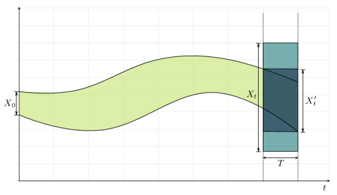
Prunefwd(Bxt,y)=Hull(Bxty(It,Bx0)).subscriptPrunefwdsubscript𝐵subscript𝑥𝑡𝑦Hullsubscript𝐵subscript𝑥𝑡𝑦subscript𝐼𝑡subscript𝐵subscript𝑥0\mathrm{Prune}_{\mathrm{fwd}}(B_{\vec{x}_{t}},\vec{y})=\operatorname{Hull}\Big{(}B_{\vec{x}_{t}}\cap\sharp\vec{y}(I_{t},B_{\vec{x}_{0}})\Big{)}.
Refer to caption
Figure 1: Forward Pruning. X0subscript𝑋0X_{0}, Xtsubscript𝑋𝑡X_{t}, t𝑡t represents the current interval assignments, and Xtsuperscriptsubscript𝑋𝑡X_{t}^{\prime} is the refined interval assignment on xtsubscript𝑥𝑡\vec{x}_{t} after pruning.
Algorithm 3 Prunefwd(y,Bx0,Bxt,It)subscriptPrunefwd𝑦subscript𝐵subscript𝑥0subscript𝐵subscript𝑥𝑡subscript𝐼𝑡\mathrm{Prune}_{\mathrm{fwd}}(\sharp{\vec{y}},B_{\vec{x_{0}}},B_{\vec{x_{t}}},I_{t})
1:Bxtϕsuperscriptsubscript𝐵subscript𝑥𝑡italic-ϕB_{\vec{x_{t}}}^{\prime}\leftarrow\phi
2:IΔt[Itl,Itl+ε]subscript𝐼Δ𝑡superscriptsubscript𝐼𝑡𝑙superscriptsubscript𝐼𝑡𝑙𝜀I_{{\Delta}t}\leftarrow[I_{t}^{l},I_{t}^{l}+{\varepsilon}]
3:while IΔtu<Itusubscriptsuperscript𝐼𝑢Δ𝑡superscriptsubscript𝐼𝑡𝑢I^{u}_{{\Delta}t}<I_{t}^{u} do
4:     BxtHull(Bxty(IΔt,Bx0))superscriptsubscript𝐵subscript𝑥𝑡Hullsuperscriptsubscript𝐵subscript𝑥𝑡𝑦subscript𝐼Δ𝑡subscript𝐵subscript𝑥0B_{\vec{x_{t}}}^{\prime}\leftarrow\operatorname{Hull}(B_{\vec{x_{t}}}^{\prime}\cup\sharp{\vec{y}}({{I_{{\Delta}t}}},B_{\vec{x_{0}}}))
5:     IΔtIΔt+εsubscript𝐼Δ𝑡subscript𝐼Δ𝑡𝜀{{I_{{\Delta}t}}}\leftarrow{I_{{\Delta}t}}+{\varepsilon}
6:end while
7:return BxtBxtsubscript𝐵subscript𝑥𝑡superscriptsubscript𝐵subscript𝑥𝑡B_{\vec{x_{t}}}\cap B_{\vec{x_{t}}}^{\prime}

Backward Pruning. Given interval assignments on xtsubscript𝑥𝑡\vec{x}_{t} and t𝑡t, we can compute a refinement of the interval assignments on x0subscript𝑥0\vec{x}_{0} using the reverse of the solution function. Figure 2 depicts backward pruning. Formally, we define the following operator:

Definition 3.8 (Backward Pruning).

Let y:[0,T]×DD:𝑦0𝑇𝐷𝐷\vec{y}:[0,T]\times D\rightarrow D be the solution functions of an ODE system, and let ysubscript𝑦\vec{y}_{-} be the reverse of y𝑦\vec{y}. Let Bx0subscript𝐵subscript𝑥0B_{\vec{x}_{0}}, Bxtsubscript𝐵subscript𝑥𝑡B_{\vec{x}_{t}}, and Itsubscript𝐼𝑡I_{t} be interval assignments on the variables x0subscript𝑥0\vec{x}_{0}, xtsubscript𝑥𝑡\vec{x}_{t}, and t𝑡t. We define the backward-pruning operator as:
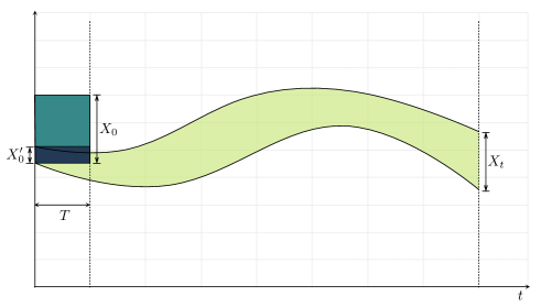
Prunebwd(Bx0,y)=Hull(Bx0y(It,Bxt)).subscriptPrunebwdsubscript𝐵subscript𝑥0𝑦Hullsubscript𝐵subscript𝑥0subscript𝑦subscript𝐼𝑡subscript𝐵subscript𝑥𝑡\mathrm{Prune}_{\mathrm{bwd}}(B_{\vec{x}_{0}},\vec{y})=\operatorname{Hull}\Big{(}B_{\vec{x}_{0}}\cap\sharp\vec{y}_{-}(I_{t},B_{\vec{x}_{t}})\Big{)}.
Refer to caption
Figure 2: Backward Pruning. X0subscript𝑋0X_{0}, Xtsubscript𝑋𝑡X_{t}, t𝑡t represents the current interval assignments, and X0superscriptsubscript𝑋0X_{0}^{\prime} is the refined interval assignment on x0subscript𝑥0\vec{x}_{0} after pruning.

Time-Domain Pruning. Given interval assignments on x0subscript𝑥0\vec{x}_{0} and xtsubscript𝑥𝑡\vec{x}_{t}, we can also refine the interval assignment on t𝑡t by pruning out the time intervals that do not contain any xtsubscript𝑥𝑡\vec{x}_{t} that is consistent with the current interval assignments on xtsubscript𝑥𝑡\vec{x}_{t}. Figure 3 depicts time-domain pruning. Formally, we define the following operator:

Definition 3.9 (Time-Domain Pruning).

Let y:[0,T]×DD:𝑦0𝑇𝐷𝐷\vec{y}:[0,T]\times D\rightarrow D be the solution functions of an ODE system. Let Bx0subscript𝐵subscript𝑥0B_{\vec{x}_{0}}, Bxtsubscript𝐵subscript𝑥𝑡B_{\vec{x}_{t}}, Itsubscript𝐼𝑡I_{t} be interval assignments on the variables x0subscript𝑥0\vec{x}_{0}, xtsubscript𝑥𝑡\vec{x}_{t}, and t𝑡t. We define the time-domain pruning operator as:
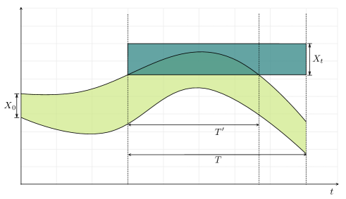
Prunetime(It,y)=Hull(It{I:y(I,Bx0)Bxt}).subscriptPrunetimesubscript𝐼𝑡𝑦Hullsubscript𝐼𝑡conditional-set𝐼𝑦𝐼subscript𝐵subscript𝑥0subscript𝐵subscript𝑥𝑡\mathrm{Prune}_{\mathrm{time}}(I_{t},\vec{y})=\operatorname{Hull}\Big{(}I_{t}\cap\{I:\sharp\vec{y}(I,B_{\vec{x}_{0}})\cap B_{\vec{x}_{t}}\not=\emptyset\}\Big{)}.
Refer to caption
Figure 3: Time-Domain Pruning. X0subscript𝑋0X_{0}, Xtsubscript𝑋𝑡X_{t}, t𝑡t represents the current interval assignments, and Tsuperscript𝑇T^{\prime} is the refined interval assignment on t𝑡t after pruning.

Overall, the pruning algorithm on based on ODE constraints iteratively applies the three pruning operators until a fixed point on the interval assignments is reached.

Algorithm 4 Prunebwd(y,Bx0,Bxt,It)subscriptPrunebwd𝑦subscript𝐵subscript𝑥0subscript𝐵subscript𝑥𝑡subscript𝐼𝑡\mathrm{Prune}_{\mathrm{bwd}}(\sharp{\vec{y}},B_{\vec{x_{0}}},B_{\vec{x_{t}}},I_{t})
1:Bx0ϕsuperscriptsubscript𝐵subscript𝑥0italic-ϕB_{\vec{x_{0}}}^{\prime}\leftarrow\phi
2:IΔt[Itl,Itl+ε]subscript𝐼Δ𝑡superscriptsubscript𝐼𝑡𝑙superscriptsubscript𝐼𝑡𝑙𝜀{{I_{{\Delta}t}}}\leftarrow[I_{t}^{l},I_{t}^{l}+{\varepsilon}]
3:while IΔtu<Itusubscriptsuperscript𝐼𝑢Δ𝑡superscriptsubscript𝐼𝑡𝑢I^{u}_{{\Delta}t}<I_{t}^{u} do
4:     Bx0Hull(Bx0y(IΔt,Bxt))superscriptsubscript𝐵subscript𝑥0Hullsuperscriptsubscript𝐵subscript𝑥0subscript𝑦subscript𝐼Δ𝑡subscript𝐵subscript𝑥𝑡B_{\vec{x_{0}}}^{\prime}\leftarrow\operatorname{Hull}(B_{\vec{x_{0}}}^{\prime}\cup\sharp{\vec{y}_{-}}({{I_{{\Delta}t}}},B_{\vec{x_{t}}}))
5:     IΔtIΔt+εsubscript𝐼Δ𝑡subscript𝐼Δ𝑡𝜀{{I_{{\Delta}t}}}\leftarrow{I_{{\Delta}t}}+{\varepsilon}
6:end while
7:return Bx0Bx0subscript𝐵subscript𝑥0superscriptsubscript𝐵subscript𝑥0B_{\vec{x_{0}}}\cap B_{\vec{x_{0}}}^{\prime}

We show the more detailed steps in the three pruning operations in Algorithm 2, 3, 4, and 5.

Algorithm 5 Prunetime(y,Bx0,Bxt,It)subscriptPrunetime𝑦subscript𝐵subscript𝑥0subscript𝐵subscript𝑥𝑡subscript𝐼𝑡\mathrm{Prune}_{\mathrm{time}}(\sharp{\vec{y}},B_{\vec{x_{0}}},B_{\vec{x_{t}}},I_{t})
1:Itϕsuperscriptsubscript𝐼𝑡italic-ϕI_{t}^{\prime}\leftarrow\phi
2:IΔt[Itl,Itl+ε]subscript𝐼Δ𝑡superscriptsubscript𝐼𝑡𝑙superscriptsubscript𝐼𝑡𝑙𝜀I_{{\Delta}t}\leftarrow[I_{t}^{l},I_{t}^{l}+{\varepsilon}]
3:while IΔtu<Itusubscriptsuperscript𝐼𝑢Δ𝑡superscriptsubscript𝐼𝑡𝑢I^{u}_{{\Delta}t}<I_{t}^{u} do
4:     Bxty(IΔt,Bx0)superscriptsubscript𝐵subscript𝑥𝑡𝑦subscript𝐼Δ𝑡subscript𝐵subscript𝑥0B_{\vec{x_{t}}}^{\prime}\leftarrow\sharp{\vec{y}}({{I_{{\Delta}t}}},B_{\vec{x_{0}}})
5:     if BxtBxtϕsuperscriptsubscript𝐵subscript𝑥𝑡subscript𝐵subscript𝑥𝑡italic-ϕB_{\vec{x_{t}}}^{\prime}\cap B_{\vec{x_{t}}}\not=\phi then
6:         It=Hull(ItIΔt)superscriptsubscript𝐼𝑡Hullsuperscriptsubscript𝐼𝑡subscript𝐼Δ𝑡I_{t}^{\prime}=\operatorname{Hull}(I_{t}^{\prime}\cup{{I_{{\Delta}t}}})
7:     else
8:         IΔtIΔt+εsubscript𝐼Δ𝑡subscript𝐼Δ𝑡𝜀I_{{\Delta}t}\leftarrow I_{{\Delta}t}+{\varepsilon}
9:     end if
10:end while
11:return Itsuperscriptsubscript𝐼𝑡I_{t}^{\prime}
Theorem 3.10.

The three pruning operators are well-defined.

Proof.

We prove that the forward pruning operator is well-defined, and the proofs for the other two operators are similar. Note that the definitions of well-defined pruning are formulated for equality constraints compared to 0. Here we use the function f=y(t,x0)xt𝑓𝑦𝑡subscript𝑥0subscript𝑥𝑡f=\vec{y}(t,\vec{x}_{0})-\vec{x}_{t} in the pruning operator. (Strictly speaking f𝑓f is a function vector that evaluates to 00\vec{0} on points satisfying the ODE flow. Here for notational simplicity we just write f𝑓f as a single-valued function and compare with the scalar 00.)

First, (W1) is satisfied because of the simple fact that for any boxes B1,B2𝔹𝔽subscript𝐵1subscript𝐵2𝔹𝔽B_{1},B_{2}\in\mathbb{BF}, we have Hull(B1B2)B1Hullsubscript𝐵1subscript𝐵2subscript𝐵1\operatorname{Hull}(B_{1}\cap B_{2})\subseteq B_{1}.

Next, suppose 0f(Prunefwd(Bxt,y)Bxt)0𝑓subscriptPrunefwdsubscript𝐵subscript𝑥𝑡𝑦subscript𝐵subscript𝑥𝑡0\not\in\sharp f(\mathrm{Prune}_{\mathrm{fwd}}(B_{\vec{x}_{t}},\vec{y})-B_{\vec{x}_{t}}). Then there does not exist any atnsubscript𝑎𝑡superscript𝑛\vec{a}_{t}\in\mathbb{R}^{n} that satisfies both atBxtsubscript𝑎𝑡subscript𝐵subscript𝑥𝑡\vec{a}_{t}\in B_{\vec{x}_{t}} and atPrunefwd(Bxt,y)subscript𝑎𝑡subscriptPrunefwdsubscript𝐵subscript𝑥𝑡𝑦\vec{a}_{t}\in\mathrm{Prune_{\mathrm{fwd}}}(B_{\vec{x}_{t}},\vec{y}). Since at the same time

Prunefwd(Bxt,y)=Hull(Bxty(It,Bx0))Bxt,subscriptPrunefwdsubscript𝐵subscript𝑥𝑡𝑦Hullsubscript𝐵subscript𝑥𝑡𝑦subscript𝐼𝑡subscript𝐵subscript𝑥0subscript𝐵subscript𝑥𝑡\mathrm{Prune}_{\mathrm{fwd}}(B_{\vec{x}_{t}},\vec{y})=\operatorname{Hull}\Big{(}B_{\vec{x}_{t}}\cap\sharp\vec{y}(I_{t},B_{\vec{x}_{0}})\Big{)}\subseteq B_{\vec{x}_{t}},

this requires that Prunefwd(Bxt,y)=subscriptPrunefwdsubscript𝐵subscript𝑥𝑡𝑦\mathrm{Prune}_{\mathrm{fwd}}(B_{\vec{x}_{t}},\vec{y})=\emptyset. Consequently (W2) is satisfied.

Third, note that y(It,Bx0)𝑦subscript𝐼𝑡subscript𝐵subscript𝑥0\sharp\vec{y}(I_{t},B_{\vec{x}_{0}}) is an interval extension of y𝑦\vec{y}. Thus, for any atnsubscript𝑎𝑡superscript𝑛\vec{a}_{t}\in\mathbb{R}^{n} such that y(t,x0)𝑦𝑡subscript𝑥0\vec{y}(t,\vec{x}_{0}) for some tIt𝑡subscript𝐼𝑡t\in I_{t} and x0Bx0subscript𝑥0subscript𝐵subscript𝑥0\vec{x}_{0}\in B_{\vec{x}_{0}}, we have aty(It,Bx0)subscript𝑎𝑡𝑦subscript𝐼𝑡subscript𝐵subscript𝑥0\vec{a}_{t}\in\sharp\vec{y}(I_{t},B_{\vec{x}_{0}}). Following the definition of the pruning operator, we have atPrunefwd(Bxt,y)subscript𝑎𝑡subscriptPrunefwdsubscript𝐵subscript𝑥𝑡𝑦\vec{a}_{t}\in\mathrm{Prune}_{\mathrm{fwd}}(B_{\vec{x}_{t}},\vec{y}). Thus, BxtZfPrunefwd(Bxt,f)subscript𝐵subscript𝑥𝑡subscript𝑍𝑓subscriptPrunefwdsubscript𝐵subscript𝑥𝑡𝑓B_{\vec{x}_{t}}\cap Z_{f}\subseteq\mathrm{Prune}_{\mathrm{fwd}}(B_{\vec{x}_{t}},f) and (W3) holds. ∎

3.3 tsuperscriptfor-all𝑡\exists\forall^{t}-Formulas and Low-Order Approximations

For for-all\exists\forall-formulas, if the universal quantification is only over the time variables, we can follow the trajectory and prune away the assignment on x0subscript𝑥0\vec{x}_{0}, xtsubscript𝑥𝑡\vec{x}_{t}, and t𝑡t that violates the constraints on the universally quantified time variable. In fact, although the extra quantification complicates the problem, the universal constraints improve the power of the pruning operations.

Here we focus on problems with one ODE system, which can be easily generalized. Let y𝑦\vec{y} denote the solution functions of an ODE system, we consider an tsuperscriptfor-all𝑡\exists\forall^{t}-formula of the form

Xx0Xxt[0,T]t[0,t]t.xt=y(t,x0)φ(y(t,x0))formulae-sequencesuperscript𝑋subscript𝑥0superscript𝑋subscript𝑥𝑡superscript0𝑇𝑡superscriptfor-all0𝑡superscript𝑡subscript𝑥𝑡𝑦𝑡subscript𝑥0𝜑𝑦superscript𝑡subscript𝑥0\displaystyle\exists^{X}\vec{x}_{0}\exists^{X}\vec{x}_{t}\exists^{[0,T]}t\forall^{[0,t]}t^{\prime}.\;\vec{x}_{t}=\vec{y}(t,\vec{x}_{0})\wedge\varphi(\vec{y}(t^{\prime},\vec{x}_{0})) (8)

Note that the problems encoded as Σ2subscriptΣ2\Sigma_{2}-SMT formulas as listed in Section 2.4 are all of this form.

We consider φ(y(t,x0))𝜑𝑦superscript𝑡subscript𝑥0\varphi(\vec{y}(t^{\prime},\vec{x}_{0})) as a special constraint on the x0subscript𝑥0\vec{x}_{0} and t𝑡t variables. Using this constraint, we can further refine the three pruning operators as follows.

Definition 3.11 (Pruning Refined by tsuperscriptfor-all𝑡\forall^{t}-Constraints).

Let y:[0,T]×Dn:𝑦0𝑇𝐷superscript𝑛\vec{y}:[0,T]\times D\rightarrow\mathbb{R}^{n} be the solution functions of an ODE system. Let Bx0subscript𝐵subscript𝑥0B_{\vec{x}_{0}}, Bxtsubscript𝐵subscript𝑥𝑡B_{\vec{x}_{t}}, and Itsubscript𝐼𝑡I_{t} be interval assignments on the variables x0subscript𝑥0\vec{x}_{0}, xtsubscript𝑥𝑡\vec{x}_{t}, and t𝑡t. Let φ(y(t,x0))𝜑𝑦superscript𝑡subscript𝑥0\varphi(\vec{y}(t^{\prime},\vec{x}_{0})) be a constraint on the universally quantified time variable, as in (8). We first define

φ(It,Bx0)=Hull({an:a=y(t,x0),tIt,x0Bx0, and φ(a) is true.})𝜑subscript𝐼𝑡subscript𝐵subscript𝑥0Hullconditional-set𝑎superscript𝑛formulae-sequence𝑎𝑦𝑡subscript𝑥0formulae-sequence𝑡subscript𝐼𝑡subscript𝑥0subscript𝐵subscript𝑥0 and 𝜑𝑎 is true.\sharp\varphi(I_{t},B_{\vec{x}_{0}})=\operatorname{Hull}(\{\vec{a}\in\mathbb{R}^{n}:\vec{a}=\vec{y}(t,\vec{x}_{0}),t\in I_{t},\\ \vec{x}_{0}\in B_{\vec{x}_{0}},\mbox{ and }\varphi(\vec{a})\mbox{ is true.}\})

and define φsubscript𝜑\sharp\varphi_{-} by replacing y𝑦\vec{y} with ysubscript𝑦\vec{y}_{-} in the definition above. The forward pruning operator with φ𝜑\varphi, written as Prunefwdφ(Bxt,y)superscriptsubscriptPrunefwd𝜑subscript𝐵subscript𝑥𝑡𝑦\mathrm{Prune}_{\mathrm{fwd}}^{\varphi}(B_{\vec{x}_{t}},\vec{y}), is defined as

Hull(Bxty(It,Bx0)φ(It,Bx0))Hullsubscript𝐵subscript𝑥𝑡𝑦subscript𝐼𝑡subscript𝐵subscript𝑥0𝜑subscript𝐼𝑡subscript𝐵subscript𝑥0\operatorname{Hull}\Big{(}B_{\vec{x}_{t}}\cap\sharp\vec{y}(I_{t},B_{\vec{x}_{0}})\cap\sharp\varphi(I_{t},B_{\vec{x}_{0}})\Big{)}

Backward pruning Prunebwdφ(Bx0,y)subscriptsuperscriptPrune𝜑bwdsubscript𝐵subscript𝑥0𝑦\mathrm{Prune}^{\varphi}_{\mathrm{bwd}}(B_{\vec{x}_{0}},\vec{y}) is defined as

Hull(Bx0y(It,Bxt)φ(It,Bxt)).Hullsubscript𝐵subscript𝑥0subscript𝑦subscript𝐼𝑡subscript𝐵subscript𝑥𝑡subscript𝜑subscript𝐼𝑡subscript𝐵subscript𝑥𝑡\operatorname{Hull}\Big{(}B_{\vec{x}_{0}}\cap\sharp\vec{y}_{-}(I_{t},B_{\vec{x}_{t}})\cap\sharp\varphi_{-}(I_{t},B_{\vec{x}_{t}})\Big{)}.

Time-domain pruning Prunetimeφ(It,y)superscriptsubscriptPrunetime𝜑subscript𝐼𝑡𝑦\mathrm{Prune}_{\mathrm{time}}^{\varphi}(I_{t},\vec{y}) is defined as

Hull(It{I:y(I,Bx0)Bxtφ(It,Bx0)}).Hullsubscript𝐼𝑡conditional-set𝐼𝑦𝐼subscript𝐵subscript𝑥0subscript𝐵subscript𝑥𝑡𝜑subscript𝐼𝑡subscript𝐵subscript𝑥0\operatorname{Hull}\Big{(}I_{t}\cap\{I:\sharp\vec{y}(I,B_{\vec{x}_{0}})\cap B_{\vec{x}_{t}}\cap\sharp\varphi(I_{t},B_{\vec{x}_{0}})\not=\emptyset\}\Big{)}.

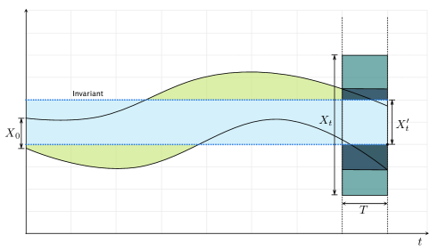
In general, φ𝜑\sharp\varphi can be computed by a recursive call to DPLL(ICP), by solving the Σ1subscriptΣ1\Sigma_{1}-SMT problem φ(x)𝜑𝑥\varphi(\vec{x}). In many practical applications, φ𝜑\varphi is of some simple form such as axtb𝑎subscript𝑥𝑡𝑏\vec{a}\leq\vec{x}_{t}\leq\vec{b}, in which case simple pruning is shown in Figure 4.
Refer to caption
Figure 4: Pruning with tsuperscriptfor-all𝑡\forall^{t}-Constraints

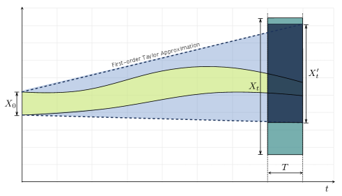
Another useful heuristic in ODE pruning is to bound the range of the derivatives for a vector space specified by g𝑔\vec{g}. Suppose for any time t[0,T]𝑡0𝑇t\in[0,T], the derivatives g𝑔\vec{g} are bounded in [lg,ug]subscript𝑙𝑔subscript𝑢𝑔[\vec{l}_{g},\vec{u}_{g}]. Then by the Picard-Lindelöf representation, we have

xt=0tg(y(s,y0))𝑑s+y0[0,T][lg,ug]+Bx0subscript𝑥𝑡superscriptsubscript0𝑡𝑔𝑦𝑠subscript𝑦0differential-d𝑠subscript𝑦00𝑇subscript𝑙𝑔subscript𝑢𝑔subscript𝐵subscript𝑥0\vec{x}_{t}=\int_{0}^{t}\vec{g}(\vec{y}(s,\vec{y}_{0}))ds+\vec{y}_{0}\in[0,T]\cdot[\vec{l}_{g},\vec{u}_{g}]+B_{\vec{x}_{0}}

We can use this formula to perform preliminary pruning on xtsubscript𝑥𝑡\vec{x}_{t}, which is especially efficient when combined with tsuperscriptfor-all𝑡\forall^{t}-constraints. Figure 5 illustrates this pruning method.
Refer to caption
Figure 5: Pruning with Low-Order Taylor Approximations

4 Experiments

Our tool dReal implements the procedures we studied for solving SMT formulas with ODEs. It is built on several existing packages, including opensmt [3] for the general DPLL(T) framework, realpaver [14] for ICP, and CAPD [1] for computing interval-enclosures of ODEs. The tool is open-source at http://dreal.cs.cmu.edu. All benchmarks and data shown here are also available on the tool website.

P #M #D #O #V delta R Time(s) Trace
AF 4 3 20 44 0.001 S 43.10 90K
AF 8 7 40 88 0.001 S 698.86 20M
AF 8 23 120 246 0.001 S 4528.13 59M
AF 8 31 160 352 0.001 S 8485.99 78M
AF 8 47 240 528 0.001 S 15740.41 117M
AF 8 55 280 616 0.001 S 19989.59 137M
CT 2 2 15 36 0.005 S 345.84 3.1M
CT 2 2 15 36 0.002 S 362.84 3.1M
EO 3 2 18 42 0.01 S 52.93 998K
EO 3 2 18 42 0.001 S 57.67 847K
EO 3 11 72 168 0.01 U 7.75
BB 2 10 22 66 0.01 S 0.25 123K
BB 2 20 42 126 0.01 S 0.57 171K
BB 2 20 42 126 0.001 S 2.21 168K
BB 2 40 82 246 0.01 U 0.27 —-
BB 2 40 82 246 0.001 U 0.26 —-
D1 3 2 9 24 0.1 S 30.84 72K
DU 3 2 6 16 0.1 U 0.04
Table 1: #M = Number of modes in the hybrid system, #D = Unrolling depth, #O = Number of ODEs in the unrolled formula, #V = Number of variables in the unrolled formula, R = Bounded Model Checking Result (delta-SAT/UNSAT) Time = CPU time (s), Trace = Size of the ODE trajectory, AF = Atrial Filbrillation, CT = Cancer Treatment, EO = Electronic Oscillator, BB = Bouncing Ball with Drag, D1,DU = Decay Model.

All experiments were conducted on a machine with a 3.4GHz octa-core Intel Core i7-2600 processor and 16GB RAM, running 64-bit Ubuntu 12.04LTS. Table 1 is a summary of the running time of the tool on various SMT formulas generated from bounded model checking hybrid systems. The formulas typically contain a large number of variables and nonlinear ODEs.
Refer to caption
Refer to caption
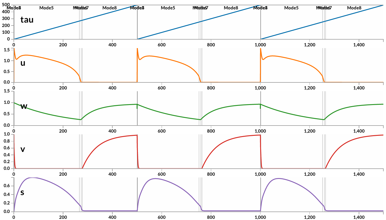
Figure 6: Above: Witness for the AF model at depth 23 and 1500 time units. Below: Experimental simulation data.

The AF model as we show in Table 1 is obtained from [15]. It is a precise model of atrial fibrillation, a serious cardiac disorder. The continuous dynamics in the model concerns four state variables and the ODEs are highly nonlinear, such as:

dudt𝑑𝑢𝑑𝑡\displaystyle\frac{du}{dt} =\displaystyle= e+(uθv)(uuu)vgfi+wsgsigso(u)𝑒𝑢subscript𝜃𝑣subscript𝑢𝑢𝑢𝑣subscript𝑔𝑓𝑖𝑤𝑠subscript𝑔𝑠𝑖subscript𝑔𝑠𝑜𝑢\displaystyle e+(u-\theta_{v})(u_{u}-u)vg_{fi}+wsg_{si}-g_{so}(u)
dsdt𝑑𝑠𝑑𝑡\displaystyle\frac{ds}{dt} =\displaystyle= gs2(1+e2k(uus))gs2ssubscript𝑔𝑠21superscript𝑒2𝑘𝑢𝑢𝑠subscript𝑔𝑠2𝑠\displaystyle\displaystyle\frac{g_{s2}}{(1+e^{-2k(u-us)})}-g_{s2}s
dvdt𝑑𝑣𝑑𝑡\displaystyle\frac{dv}{dt} =\displaystyle= gv+vdwdt=gw+wsuperscriptsubscript𝑔𝑣𝑣𝑑𝑤𝑑𝑡superscriptsubscript𝑔𝑤𝑤\displaystyle-g_{v}^{+}\cdot v\ \ \ \ \frac{dw}{dt}=-g_{w}^{+}\cdot w

The exponential term on the right-hand side of the ODE is the sigmoid function, which often appears in modelling biological switches. On this model, our tool is able to perform a depth-55 unrolling, and solve the generated logic formula. Such a formula contains 280 nonlinear ODEs of the type shown here, with 616 variables. The computed trace from dReal suggests a witness of the reachability property that can be confirmed by experimental simulation. Figure 6 shows the comparison between the trace computed from bounded model checking and the actual experimental simulation trace.
Refer to caption
Refer to caption
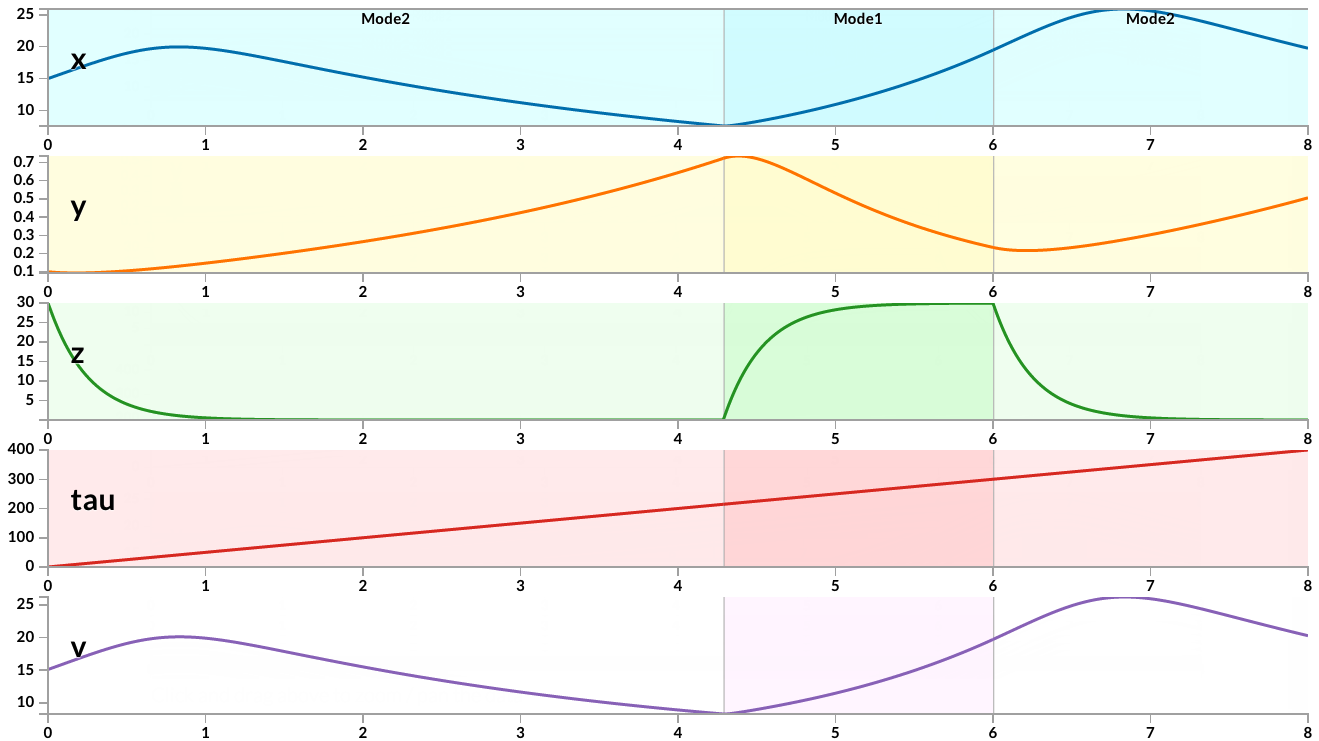
Figure 7: Above: Witness computed for the CT model at depth 3 and 500 time units. Below: Experimental simulation data.

The CT model represents a prostate cancer treatment model that contains nonlinear ODEs such as following:

dxdt𝑑𝑥𝑑𝑡\displaystyle\frac{dx}{dt} =\displaystyle= (αx(k1+(1k1)zz+k2\displaystyle(\alpha_{x}(k_{1}+(1-k_{1})\frac{z}{z+k_{2}}
βx((1k3)zz+k4+k3))m1(1zz0))x+c1x\displaystyle-\beta_{x}((1-k_{3})\frac{z}{z+k_{4}}+k_{3}))-m_{1}(1-\frac{z}{z_{0}}))x+c_{1}x
dydt𝑑𝑦𝑑𝑡\displaystyle\frac{dy}{dt} =\displaystyle= m1(1zz0)x+(αy(1dzz0)βy)y+c2ysubscript𝑚11𝑧subscript𝑧0𝑥subscript𝛼𝑦1𝑑𝑧subscript𝑧0subscript𝛽𝑦𝑦subscript𝑐2𝑦\displaystyle m_{1}(1-\frac{z}{z_{0}})x+(\alpha_{y}(1-d\frac{z}{z_{0}})-\beta_{y})y+c_{2}y
dzdt𝑑𝑧𝑑𝑡\displaystyle\frac{dz}{dt} =\displaystyle= zτ+c3z𝑧𝜏subscript𝑐3𝑧\displaystyle\frac{-z}{\tau}+c_{3}z
dvdt𝑑𝑣𝑑𝑡\displaystyle\frac{dv}{dt} =\displaystyle= (αx(k1+(1k1)zz+k2βx(k3+(1k3)zz+k4))\displaystyle(\alpha_{x}(k_{1}+(1-k_{1})\frac{z}{z+k_{2}}-\beta_{x}(k_{3}+(1-k_{3})\frac{z}{z+k_{4}}))
m1(1zz0))x+c1x+m1(1zz0)x\displaystyle-m_{1}(1-\frac{z}{z_{0}}))x+c_{1}x+m_{1}(1-\frac{z}{z_{0}})x
+(αy(1dzz0)βy)y+c2ysubscript𝛼𝑦1𝑑𝑧subscript𝑧0subscript𝛽𝑦𝑦subscript𝑐2𝑦\displaystyle+(\alpha_{y}(1-d\frac{z}{z_{0}})-\beta_{y})y+c_{2}y

The EO model represents an electronic oscillator model that contains nonlinear ODEs such as the following:

dxdt𝑑𝑥𝑑𝑡\displaystyle\frac{dx}{dt} =\displaystyle= axsin(ω1τ)𝑎𝑥𝑠𝑖𝑛subscript𝜔1𝜏\displaystyle-ax\cdot sin(\omega_{1}\cdot\tau)
dydt𝑑𝑦𝑑𝑡\displaystyle\frac{dy}{dt} =\displaystyle= aysin((ω1+c1)τ)sin(ω2)2𝑎𝑦𝑠𝑖𝑛subscript𝜔1subscript𝑐1𝜏𝑠𝑖𝑛subscript𝜔22\displaystyle-ay\cdot sin((\omega_{1}+c_{1})\cdot\tau)\cdot sin(\omega_{2})\cdot 2
dzdt𝑑𝑧𝑑𝑡\displaystyle\frac{dz}{dt} =\displaystyle= azsin((ω2+c2)τ)cos(ω1)2𝑎𝑧𝑠𝑖𝑛subscript𝜔2subscript𝑐2𝜏𝑐𝑜𝑠subscript𝜔12\displaystyle-az\cdot sin((\omega_{2}+c_{2})\cdot\tau)\cdot cos(\omega_{1})\cdot 2
ω1dtsubscript𝜔1𝑑𝑡\displaystyle\frac{\omega_{1}}{dt} =\displaystyle= c3ω1ω2dt=c4ω2dτdt=1formulae-sequencesubscript𝑐3subscript𝜔1subscript𝜔2𝑑𝑡subscript𝑐4subscript𝜔2𝑑𝜏𝑑𝑡1\displaystyle-c_{3}\cdot\omega_{1}\ \ \ \frac{\omega_{2}}{dt}=-c_{4}\cdot\omega_{2}\ \ \ \frac{d\tau}{dt}=1

The other models are standard simple nonlinear models (for instance, bouncing ball with nonlinear friction), on which our tool has no difficulty in solving.

5 Conclusion

In this paper we have studied SMT problems over the real numbers with ODE constraints. We have developed δ𝛿\delta-complete algorithms in the DPLL(ICP) framework, for both the standard SMT formulas that are purely existentially quantified, as well as for-all\exists\forall-formulas whose universal quantification is restricted to the time variables. We have demonstrated the scalability of our approach on nonlinear SMT benchmarks. We believe that the proposed decision procedures can scale on nonlinear problems and can serve as the underlying engine for formal verification of realistic hybrid systems and embedded software.

Ackowledgements. We are grateful for many important suggestions from Jeremy Avigad, Andreas Eggers, and Martin Fränzle. In particular, we formulated the notion of δ𝛿\delta-regular interval extensions to avoid technical difficulties that Eggers and Fränzle pointed out to us. We thank the anonymous referees for various important comments.

References

  • [1] CAPD: Computer assisted proofs in dynamical systems. http://capd.ii.uj.edu.pl/index.php.
  • [2] F. Benhamou and L. Granvilliers. Continuous and interval constraints. In F. Rossi, P. van Beek, and T. Walsh, editors, Handbook of Constraint Programming, chapter 16. Elsevier, 2006.
  • [3] R. Bruttomesso, E. Pek, N. Sharygina, and A. Tsitovich. The opensmt solver. In J. Esparza and R. Majumdar, editors, TACAS, volume 6015 of Lecture Notes in Computer Science, pages 150–153. Springer, 2010.
  • [4] A. Cimatti, S. Mover, and S. Tonetta. A quantifier-free SMT encoding of non-linear hybrid automata. In FMCAD, pages 187–195, 2012.
  • [5] A. Cimatti, S. Mover, and S. Tonetta. SMT-based verification of hybrid systems. In AAAI, 2012.
  • [6] J. Cruz and P. Barahona. Constraint satisfaction differential problems. In CP, pages 259–273, 2003.
  • [7] A. Eggers, M. Fränzle, and C. Herde. SAT modulo ODE: A direct SAT approach to hybrid systems. In ATVA, pages 171–185, 2008.
  • [8] A. Eggers, N. Ramdani, N. Nedialkov, and M. Fränzle. Improving SAT modulo ODE for hybrid systems analysis by combining different enclosure methods. In G. Barthe, A. Pardo, and G. Schneider, editors, SEFM, volume 7041 of Lecture Notes in Computer Science, pages 172–187. Springer, 2011.
  • [9] S. Gao, J. Avigad, and E. M. Clarke. Delta-complete decision procedures for satisfiability over the reals. In B. Gramlich, D. Miller, and U. Sattler, editors, IJCAR, volume 7364 of Lecture Notes in Computer Science, pages 286–300. Springer, 2012.
  • [10] S. Gao, J. Avigad, and E. M. Clarke. Delta-decidability over the reals. In LICS, pages 305–314, 2012.
  • [11] S. Gao, S. Kong, and E. Clarke. dReal: An SMT solver for nonlinear theories over the reals. CADE, 2013.
  • [12] A. Goldsztejn, O. Mullier, D. Eveillard, and H. Hosobe. Including ordinary differential equations based constraints in the standard cp framework. In D. Cohen, editor, CP, volume 6308 of Lecture Notes in Computer Science, pages 221–235. Springer, 2010.
  • [13] L. Granvilliers. Parameter estimation using interval computations. SIAM J. Sci. Comput., 26(2):591–612, Feb. 2005.
  • [14] L. Granvilliers and F. Benhamou. Algorithm 852: Realpaver: an interval solver using constraint satisfaction techniques. ACM Trans. Math. Softw., 32(1):138–156, 2006.
  • [15] R. Grosu, G. Batt, F. H. Fenton, J. Glimm, C. L. Guernic, S. A. Smolka, and E. Bartocci. From cardiac cells to genetic regulatory networks. In CAV, pages 396–411, 2011.
  • [16] D. Ishii, K. Ueda, and H. Hosobe. An interval-based sat modulo ode solver for model checking nonlinear hybrid systems. STTT, 13(5):449–461, 2011.
  • [17] K.-I. Ko. Complexity Theory of Real Functions. BirkHauser, 1991.
  • [18] Y. Lin and M. A. Stadtherr. Guaranteed state and parameter estimation for nonlinear continuous-time systems with bounded-error measurements. Industrial and Engineering Chemistry Research, pages 7198–7207, 2007.
  • [19] K. Weihrauch. Computable Analysis: An Introduction. 2000.