Numerical Methods for Linear Diffusion Equations in the Presence of an Interface

Abstract:

We consider numerical methods for linear parabolic equations in one spatial dimension having piecewise constant diffusion coefficients defined by a one parameter family of interface conditions at the discontinuity. We construct immersed interface finite element methods for an alternative formulation of the original deterministic diffusion problem in which the interface condition is recast as a natural condition on the interfacial flux for which the given operator is self adjoint. An Euler-Maruyama method is developed for the stochastic differential equation corresponding to the alternative divergence formulation of the equation having a discontinuous coefficient and a one-parameter family of interface conditions. We then prove convergence estimates for the Euler scheme. The main goal is to develop numerical schemes that can accommodate specification of any one of the possible interface conditions, and to illustrate the implementation for each of the deterministic and stochastic formulations, respectively. The issues pertaining to speed-ups of the numerical schemes are left to future work.

Keywords: Diffusion, divergence form operators, discontinuous coefficients, interface conditions, Immersed Interface methods, stochastic differential equations, Euler-Maruyama method.

AMS Classification: (primary): 60H10, 65U05; (Secondary): 65C05, 60J30, 60E07, 65R20

1 Introduction

The computational simulation of solutions to diffusion equations in heterogeneous materials or landscapes requires the use of highly efficient numerical methods which are consistent, stable, and potentially have high orders of accuracy. Discontinuities in parameters may decrease the overall accuracy of the method if not handled appropriately. The correct discretization at the interface depends on the type of interface condition imposed by the problem.

In diffusion models the transmission properties may be coupled to physically discrete, discontinuous properties of the environment such as river networks [7] or landscape topography and meteorological conditions [32, 35, 25, 24, 29]. Diffusion equations provide one of the standard approaches to modeling population dynamics with dispersal in spatially patchy environments [36, 9]. There are a number of empirical studies which indicate that the dispersal behavior of individuals, such as species of insects including aphids, beetles and caterpillar, foraging honey bees as well as several species of butterflies, is influenced by boundaries (interfaces) between different types of habitats (patches) [34, 39, 33, 1].

In recent work on interfacial effects [4, 3, 5], the authors analyze the underlying stochastic process determined by the equation in divergence form and having a specific interfacial condition in the presence of discontinuities in diffusion coefficients across interfaces. The theory of Brownian motion applies to diffusion models in homogeneous media with constant coefficients [10]. However, the discontinuity in the diffusion tensor at the interface between two media ‘skews’ the basic particle motion. Incorporating bias in behavior/movement at an interface or patch boundary into diffusion models naturally leads to Skew Brownian Motion (SBM) [15, 40, 14, 8], from which the underlying stochastic particle motions across the discontinuity, called $\alpha$-skew diffusion, can be constructed [4]. SBM assumes that particles (individuals) move according to ordinary diffusion until they encounter an interface, but at an interface the probability that a particle (individual) will move into the region on one side of the interface is different than the chance that it will move into the region on the other side; see [8] for the case of conservative interface conditions.

The basic idea to be developed in the present article to deal with more general specifications of interface conditions (than the conservative case) can be used in either deterministic or stochastic numerical framework. Thus we have elected to present numerical approaches to both the deterministic and the stochastic equations in this single article. Readers may be selective in this regard since the deterministic and stochastic methods are treated independently up to sharing common notation where possible. The key idea that used for both approaches is a change of variables that transforms the given problem into one that involves a natural continuity of flux interface condition, rendering the problem self-adjoint, i.e., a form of symmetrization.

For the numerical simulation of diffusion equations with discontinuous coefficients involving special interface conditions we will develop immersed interface methods for the spatial discretization that have been recently formulated for elliptic problems [19, 22, 21, 20, 41, 30, 44, 43]. For the time discretization we use implicit finite difference schemes such as Backward Euler and the Crank-Nicolson method. Here we present error estimates for the semi-discrete (continuous in time) problem with immersed finite element for the spatial discretization as well as error estimates for the fully discrete scheme.

In our previous work [4] an equivalent formulation in terms of solutions to stochastic differential equations in which the effect of the interface is reflected in an added drift rate involving the local time [3] of the process (the stochastic counterpart of the interface condition) was developed. The numerical simulation of SDEs corresponding to divergence form operators involving a discontinuous coefficient has also been the subject of various articles in the recent past. In the one-dimensional context, schemes based on random walks [11, 17, 18, 16], Euler methods [26] (based on stochastic Taylor expansions) and [27], and exact simulation methods [12] have been developed for the simulation of the solution of such SDEs for the case of conservative (self-adjoint) interface conditions.

The paper is organized as follows. We first introduce a natural one parameter family of possible interface conditions coupled to a diffusion problem, with discontinuous diffusion coefficient, in one spatial dimension (Section 2). Motivating areas of application from the engineering, ecological and biological sciences are briefly noted. We then present a reformulation of the problem which naturally allows the application of finite element methods, where the immersed interface method is used to ensure that the basis functions satisfy the reformulated interface condition (Section 3). We recall standard estimates for the elliptic problem and then apply them to the case in question. We consider both backward Euler and Crank-Nicolson methods for time discretization. We provide error estimates for the fully discrete scheme with backward Euler time discetization and verify rates with numerical examples. Next, we introduce the corresponding stochastic differential equation and develop the Euler- Maruyama scheme for numerical solutions applicable to any one of the interface conditions (Section 5). We prove convergence of the Euler-Maruyama scheme under mild assumptions using the approach developed in [27]. Finally, numerical simulations are provided that illustrate our theoretical results in Sections 4 and 6.

2 Diffusion with Discontinuous Coefficients

We consider the time dependent diffusion equation in one dimension with a piecewise discontinuous diffusion coefficient across an interface at $x=0$ on which a one parameter family of interface conditions is prescribed. We define the time interval $J=[0,T]$ and the domain $\Omega=\mathbb{R}$. The corresponding initial value problem on $\Omega\times J$ is given as

$${\frac{\partial u}{\partial t}}(t,x) ={\frac{\partial}{\partial x}}\left(\frac{D(x)}{2}{\frac{\partial u(t,x)}{\partial x}}\right),\quad\forall x\in\Omega,\ t\in J\setminus\{0\},$$ (2.1a)

$$u(t,0^{+}) =u(t,0^{-}),\forall\ t\in J,$$ (2.1b)

$$\lambda{\frac{\partial u}{\partial x}}(t,0^{+}) =(1-\lambda){\frac{\partial u}{\partial x}}(t,0^{-}),\ \forall\ t\in J,$$ (2.1c)

$$u(0,x) =u_{0}(x),\forall\ x\in\Omega.$$ (2.1d)

In model (2.1) the diffusion coefficient $D$ is piecewise defined by

$$D(x)=\begin{cases}D^{+}&\mbox{if }x>0,\\ D^{-}&\mbox{if }x<0,\end{cases}$$ (2.2)

for some positive constants $D^{+},D^{-}$. We assume initial data $u(0,x)=u_{0}(x)$ given for all $x\in\Omega$ in equation (2.1d). Continuity of the solution $u(t,x)$ at the interface $x=0$ given in (2.1b), as well as a condition at $x=0$ given in (2.1c) that depends on a parameter $\lambda$ with $0<\lambda<1$, and involves the derivative of the solution, specify the nature of the interface. The choice of the value of $\lambda$ varies according to the application, and may be a function of $D^{+}$ and $D^{-}$.

Remark 2.1

One may note that the extreme cases in which $\lambda=0,1$, respectively, correspond to Neumann boundary conditions at the point of interface. In particular, therefore the coefficients are purely constant (smooth) on the corresponding half-line and amenable to standard approaches to Neumann boundary value problems. From this perspective there is no loss to restricting considerations to $0<\lambda<1$.

From the point of view of applications to environmental sciences, the cases of $\lambda=\lambda^{*}:={D^{+}\over D^{+}+D^{-}}$ (continuity of flux), $\lambda=\lambda^{\#}:=1/2$ (continuity of derivatives), and $\lambda=0$, arise as solute transport interfaces [4, 2], upwelling of ocean current modeling [28], and one-sided barrier (reflective) regions, respectively. There are ecological species, example Fender’s blue butterfly, and aphids for which inter-facial effects are widely reported from experiments, but the precise interface condition is unknown from a mathematical perspective. e.g., see [34, 39]. For the latter, the problem of determining $\lambda$ can also be treated as a statistical problem.

2.1 Reformulated (Symmetrized) Model

In order to setup the problem for easy application of the deterministic and stochastic numerical methods, it is convenient to relate the parameter $\lambda$ in the interface condition (2.1c) to one which appears in a reformulation of problem (2.1) written in self-adjoint form. We do this via multiplication of both sides of the PDE in (2.1a) by a piecewise defined (positive) function

$$c(x)=\begin{cases}c^{+}:=\lambda/D^{+}&\mbox{if }x>0,\\ c^{-}:=(1-\lambda)/D^{-}&\mbox{if }x<0.\end{cases}$$ (2.3)

The resulting PDE can be written

$$c(x){\frac{\partial u}{\partial t}}={\frac{\partial}{\partial x}}\left(\kappa(x){\frac{\partial u}{\partial x}}\right),\quad\forall x\in\Omega,t\in J\setminus\{0\},$$ (2.4)

where the positive function $\kappa$ is defined as

$$\kappa(x)=c(x)\frac{D(x)}{2}=\begin{cases}\kappa^{+}:=\frac{\lambda}{2}&\mbox{if }x>0,\\ \kappa^{-}:=\frac{(1-\lambda)}{2}&\mbox{if }x<0.\end{cases}$$ (2.5)

Thus, the interface condition (2.1c) may be interpreted as

$$\left[\kappa{\frac{\partial u}{\partial x}}\right]:=\kappa^{+}{\frac{\partial u}{\partial x}}(t,0^{+})-\kappa^{-}{\frac{\partial u}{\partial x}}(t,0^{-})=0,$$ (2.6)

i.e., the jump across the interface of $\kappa{\frac{\partial u}{\partial x}}$ at $x=0$, denoted as$\left[\kappa{\frac{\partial u}{\partial x}}\right]$, is zero. Thus, problem (2.1) can be reformulated to have an interface condition that resembles a natural flux condition (conservative) which is more easily amenable to numerical discretization. The reformulated version of problem (2.1) on $\Omega=\mathbb{R}$ can be stated as

$$c(x){\frac{\partial u}{\partial t}}(t,x) ={\frac{\partial}{\partial x}}\left(\kappa(x){\frac{\partial u(t,x)}{\partial x}}\right),\quad\forall x\in\Omega,\ t\in J\setminus\{0\},$$ (2.7a)

$$\left[u\right] :=u(t,0^{+})-u(t,0^{-})=0,\ \forall\ t\in J,$$ (2.7b)

$$\left[\kappa{\frac{\partial u}{\partial x}}\right] :=\kappa^{+}{\frac{\partial u}{\partial x}}(t,0^{+})-\kappa^{-}{\frac{\partial u}{\partial x}}(t,0^{-})=0,\ \forall\ t\in J,$$ (2.7c)

$$u(0,x) =u_{0}(x),\forall x\in\Omega.$$ (2.7d)

Remark 2.2

We note that $c$ plays the role of specific heat capacity times mass density of the material, and $\kappa$ is a thermal conductivity, in the context of heat flow. We observe that for the special case of $\lambda=\lambda^{*}:=D^{+}/(D^{+}+D^{-})$ we have that $c(x)\equiv\mbox{\em constant}$.

3 The Immersed Finite Element Method (IFEM)

To construct a discrete solution of the problem (2.7) and to generate numerical simulations we will need to consider problem (2.1) and hence problem (2.7) on a finite interval. Thus, in this section we will formulate problem (2.7) on the domain $\Omega:=(-L,L)$ for $L>0,L\in\mathbb{R}$. In order for problem (2.1) and problem (2.7) to be well-posed on $\Omega$ we will impose the boundary conditions

$$u(t,-L)=u(t,L)=0,\ \forall\ t\in J,$$ (3.1)

on the boundary of $\Omega$.

There are several numerical approaches available for the spatial discretization of parabolic interface problems like problem (2.7) along with (3.1). These include domain embedding methods like the fictitious domain method [13, 42], implicit derivative matching methods [44], immersed boundary methods [31] and immersed interface methods based on either finite differences [21, 22] or finite element methods [20]. In this paper we consider the immersed finite element method (IFEM), which is a numerical techinique based on the finite element method (FEM) for spatially discretizing problem (2.7) along with (3.1). Like FEM the IFEM is based on a variational formulation of the initial boundary value problem (2.7) along with (3.1). However, unlike the FEM the spatial mesh of the IFEM can be constructed independently of the interface. Also, unlike the FEM, some of the basis functions in the IFEM depend on the interface location at $x=0$ and the interface jump conditions (2.7b) and (2.7c). We refer the reader to [22] for further details.

3.1 Functional Spaces and the Variational Formulation

We define the sub-domains $\Omega_{1}=(-L,0)$ and $\Omega_{2}=(0,L)$, so that $\Omega=\Omega_{1}\cup\Omega_{2}\cup\{0\}$, For $m>0$ and $1\leq p\leq\infty$, $H^{m}(\Omega)$ is the Sobolev space of order $m$ with norm $||\cdot||_{H^{m}(\Omega)}$ and for $m=0$, $H^{0}(\Omega)\equiv L^{2}(\Omega)$ with norm $||\cdot||_{L^{2}(\Omega)}$. For $k\geq 0$ we define the functional spaces

$$H^{k,0}(\Omega) =\{v\in L^{2}(\Omega)\ |\ v\in H^{k}(\Omega_{1})\cap H^{k}(\Omega_{2}),[v]=0,[\kappa{\frac{\partial v}{\partial x}}]=0\},$$ (3.2)

$$H_{0}^{k,0}(\Omega) =\{v\in H^{k,0}(\Omega)\ |\ v(-L)=v(L)=0\},$$ (3.3)

along with the norm

$$||v||^{2}_{H^{k,0}(\Omega)}:=\left(||v||^{2}_{H^{k}(\Omega_{1})}+||v||^{2}_{H^{k}(\Omega_{2})}\right),$$ (3.4)

where $H^{k}(\Omega)$ and $H^{k}_{0}(\Omega)$ are the usual Sobolev spaces for $k\geq 1$. On $H^{k}(\Omega)$ we also define the seminorm $|v|_{H^{k}(\Omega)}:=||\frac{\partial^{k}v}{\partial x^{k}}||_{L^{2}(\Omega)}$ and recall that for functions in $H^{1}_{0}(\Omega)$, the norms $||v||_{H^{1}(\Omega)}$ and $|v|_{H^{1}(\Omega)}$ are equivalent due to Friedrichs’ lemma [38]. The (semi) norms $|v|_{H^{k,0}(\Omega)}$ are defined in a similar manner to (3.4). For a normed vector space $X$ and for $1\leq p\leq\infty$ we define the Lebesgue space $L^{p}(0,T;X)$ to be the space of all $X$ valued functions $v:J\rightarrow X$ for which $t\rightarrow||v(t)||_{X}$ is in the Banach space $L^{p}(J)$ equipped with the norm

$$||v||_{L^{p}(X)}=\begin{cases}\left(\int_{0}^{T}||v(t)||^{p}_{X}dt\right)^{\frac{1}{p}},&\text{if}\ p<\infty\\ {\underset{t\in J}{\mathrm{ess\ sup}}}||v(t)||_{X},&\text{if}\ p=\infty.\end{cases}$$ (3.5)

On the space $L^{p}(0,T;H^{2,0}(\Omega)\cap H_{0}^{1}(\Omega))$ we will also define the (semi) norm $|v|_{L^{p}(H^{2,0}(\Omega))}$ in a similar manner to (3.5) using the seminorm $|v|_{H^{2,0}(\Omega)}$ on $H^{2,0}(\Omega)\cap H_{0}^{1}(\Omega))$. We define the operator $\mathcal{L}$ as

$$\begin{split}&\mathcal{L}:C^{0}([0,1];H_{0}^{1,0}(\Omega))\times H_{0}^{1,0}(\Omega)\rightarrow C^{0}([0,1];\mathbb{R});\\ &\mathcal{L}(u,v)=\int_{\Omega}\kappa(x){\frac{\partial u(t)}{\partial x}}{\frac{\partial v}{\partial x}}dx=\int_{\Omega^{-}}\kappa^{-}{\frac{\partial u(t)}{\partial x}}{\frac{\partial v}{\partial x}}dx+\int_{\Omega^{+}}\kappa^{+}{\frac{\partial u(t)}{\partial x}}{\frac{\partial v}{\partial x}}dx.\end{split}$$ (3.6)

The variational formulation corresponding to problem (2.7) along with (3.1) is:
Find $u:J\longrightarrow H_{0}^{1,0}(\Omega)$ such that

$$\int_{\Omega}c(x){\frac{\partial u(t)}{\partial t}}vdx+\mathcal{L}(u,v)=0,\ \forall v\in H_{0}^{1,0}(\Omega).$$ (3.7)

3.2 Spatial Discretization Using Immersed Finite Elements

We partition $\overline{\Omega}=[-L,L]$ using a uniform mesh

$$-L=x_{0}<x_{1}<x_{2}<\ldots<x_{N}=L.$$

We define the mesh step size, $h_{i}:=x_{i}-x_{i-1}$, to be a constant $h$ for all subintervals in the partition $i=1,2,\ldots,N$. The discrete mesh is then denoted $\tau_{h}={\underset{i=0}{\overset{N-1}{\bigcup E_{i}}}}$ with $E_{i}=[x_{i},x_{i+1}]$.

At every node $x_{i}$ we define basis functions $\phi_{j}(x)$ as

$$\phi_{j}(x_{i})=\begin{cases}1,&i=j,\\ 0,&i\neq j,\end{cases}$$ (3.8)

satisfying the interface conditions $[\phi_{j}]=0$ and $[\kappa\phi_{j}^{\prime}]=0$. We consider the linear IFE space

$$S_{h}^{1}(\Omega)=\text{span}\{\phi_{j}\}_{j=1}^{N-1}.$$ (3.9)

Since $\forall j,\phi_{j}\in H^{1,0}(\Omega)$, we have that $S_{h}^{1}(\Omega)\subset H^{1,0}(\Omega)$. Let $x_{j}<0<x_{j+1}$, for some $j$, then the basis functions $\phi_{j}$ and $\phi_{j+1}$ are the only ones that need to be modified to satisfy the flux jump condition. This modification can be made using the method of undetermined coefficients as is done in [20]. We refer the reader to [23, 20] for the construction of the IFE basis functions $\phi_{j}$.

3.2.1 Interpolation Functions and Error Estimates

To derive the error estimates for the time dependent problem (2.7) along with (3.1), we will use the error analysis derived for the corresponding stationary problem in [20, 23] which is outlined below. Consider the stationary problem :

$$-{\frac{\partial}{\partial x}}\left(\kappa(x){\frac{\partial u(t,x)}{\partial x}}\right) =f(x),\ \forall x\in\Omega,$$ (3.10a)

$$[u]:=u(0^{+})-u(0^{-}) =0,$$ (3.10b)

$$\left[\kappa{\frac{\partial u}{\partial x}}\right]:=\kappa^{+}{\frac{\partial u}{\partial x}}(0^{+})-\kappa^{-}{\frac{\partial u}{\partial x}}(0^{-}) =0,$$ (3.10c)

$$u(-L)=u(L) =0,$$ (3.10d)

with $f\in L^{2}(\Omega)$. We define the linear functional $\ell$ as

$$\ell:C^{0}([0,1];H_{0}^{1,0}(\Omega))\rightarrow C^{0}([0,1];\mathbb{R});\ \ell(u)=\int_{\Omega}fudx.$$ (3.11)

The weak form of problem (3.10) is:
Find $u\in H_{0}^{1,0}(\Omega)$ such that

$$\mathcal{L}(u,v)=(f,v),\forall\ v\in H_{0}^{1,0}(\Omega).$$ (3.12)

The discrete variational problem using immersed finite elements is:
Find $u_{h}\in S_{h,0}^{1}:=S_{h}^{1}(\Omega)\cap H_{0}^{1,0}(\Omega)$ such that

$$\mathcal{L}(u_{h},v_{h})=(f,v_{h}),\forall\ v_{h}\in S_{h,0}^{1}(\Omega).$$ (3.13)

Based on the estimates for the interpolants error estimates for the IFE solutions are derived in [20, 23].

Theorem 3.1 (Theorem 4 from [23])

Let $u\in H^{2,0}(\Omega)\cap H_{0}^{1,0}(\Omega)$ and $u_{h}\in S_{h,0}^{1}(\Omega)\subset H^{1,0}_{0}(\Omega)$ be solutions to (3.12) and (3.13), respectively. Then $\exists$ a positive constant $C$ independent of $u$ and $h$ such that

$$||u-u_{h}||_{H^{0,0}(\Omega)}+h||u-u_{h}||_{H^{1,0}(\Omega)}\leq C\rho h^{2}|u|_{H^{2,0}(\Omega)},$$ (3.14)

where $\rho:=\mathrm{max}\{\displaystyle\frac{\kappa^{-}}{\kappa^{+}},\displaystyle\frac{\kappa^{+}}{\kappa^{-}}\}$.

Theorem 3.2 (Theorem 3.4 from [20])

Let $u\in H^{2,0}(\Omega)\cap H_{0}^{1,0}(\Omega)$ and $u_{h}\in S_{h,0}^{1}(\Omega)\subset H^{1,0}_{0}(\Omega)$ be solutions to (3.12) and (3.13), respectively. Then $\exists$ a positive constant $\bar{C}$ independent of $u$ and $h$ such that

$$||u-u_{h}||_{L^{\infty}(\Omega)}\leq\bar{C}h^{2}||\frac{\partial^{2}u}{\partial x^{2}}||_{L^{\infty}(\Omega)},$$ (3.15)

where $\bar{C}=\displaystyle\frac{2\mathrm{max}\{1,\rho\}}{\mathrm{min}\{1,\rho\}}+\displaystyle\frac{3}{2}$, and $\rho$ as defined in Theorem 3.1.

3.3 Semi-Discrete Schemes: The Continuous Time Galerkin Immersed Finite Element Problem

We now study the convergence properties of a semi-discrete scheme applied to the time dependent problem (2.7) obtained by spatially discretizing the problem using IFEM. Denoting the $L^{2}(\Omega)$ inner product as $(\cdot,\cdot)$ the weak formulation of the semi-discrete IFEM problem based on (3.7) is
Find $u_{h}:J\longrightarrow S_{h,0}^{1}(\Omega)$ such that

$$(c{\frac{\partial u_{h}}{\partial t}}(t),v_{h})+\mathcal{L}(u_{h},v_{h})=0,\ \forall v_{h}\in S_{h,0}^{1}(\Omega).$$ (3.16)

Let $u(t)\in H^{2,0}(\Omega)\cap H_{0}^{1,0}(\Omega)$ for $t\in J\setminus\{0\}$ be the solution to (3.7). The elliptic projection $P_{h}u$ is defined to be the solution to the auxilliary problem:

Find $P_{h}u:J\longrightarrow S_{h,0}^{1}(\Omega)$ such that $\forall v_{h}\in S_{h,0}^{1}(\Omega),\forall\ t\in J$,

$$\mathcal{L}(u(t)-P_{h}u(t),v_{h})=0;\implies\ \int_{\Omega}\kappa{\frac{\partial u(t)}{\partial x}}{\frac{\partial v_{h}}{\partial x}}dx=\int_{\Omega}{\frac{\partial P_{h}u(t)}{\partial x}}{\frac{\partial v_{h}}{\partial x}}dx;$$ (3.17)

In addition we have $\forall v_{h}\in S_{h,0}^{1}(\Omega),\forall\ t\in J$,

$$\mathcal{L}({\frac{\partial u}{\partial t}}(t)-{\frac{\partial(P_{h}u)}{\partial t}}(t),v_{h})=0;\implies\ \int_{\Omega}\kappa{\frac{\partial}{\partial x}}\left({\frac{\partial u(t)}{\partial t}}\right){\frac{\partial v_{h}}{\partial x}}dx=\int_{\Omega}{\frac{\partial}{\partial x}}\left({\frac{\partial P_{h}u(t)}{\partial t}}\right){\frac{\partial v_{h}}{\partial x}}dx;$$ (3.18)

Thus, ${\frac{\partial P_{h}u}{\partial t}}(t)$ is the elliptic projection of ${\frac{\partial u}{\partial t}}(t),\forall t\in J$. We have the following result

Theorem 3.3

Let $\forall\ t\in J$, $u(t)\in H^{2,0}(\Omega)\cap H_{0}^{1,0}(\Omega)$, and $u_{h}(t)\in S_{h,0}^{1}(\Omega)$, be the solutions to problems (3.7), and (3.16) respectively. Then $\exists$ a positive constant $C$ such that

$$||u-u_{h}||_{L^{\infty}(L^{2}(\Omega))}\leq||(u-u_{h})(0)||_{L^{2}(\Omega)}+C\rho h^{2}\left[|u|_{L^{\infty}(H^{2,0}(\Omega))}+\alpha_{1}|{\frac{\partial u}{\partial t}}|_{L^{1}(H^{2,0}(\Omega))}\right],$$ (3.19)

where

$$\alpha_{1}=\displaystyle\frac{\mathrm{max}\{c^{+},c^{-}\}}{\mathrm{min}\{c^{+},c^{-}\}}$$ (3.20)

and $\rho$ is defined in Theorem 3.1

Proof. The proof is quite standard and we just give the salient details here. We refer the reader to [38] for details on similar proofs. We split the error into two parts

$$u(t)-u_{h}(t)=(u-P_{h}u)(t)+(P_{h}u-u_{h})(t)=\eta(t)+\xi(t).$$ (3.21)

From Theorem 3.1 we have $\forall\ t\in J$

$$||\eta(t)||_{L^{2}(\Omega)} \leq C\rho h^{2}|u(t)|_{H^{2,0}(\Omega)},$$ (3.22)

$$||{\frac{\partial\eta}{\partial t}}(t)||_{L^{2}(\Omega)} \leq C\rho h^{2}|{\frac{\partial u}{\partial t}}(t)|_{H^{2,0}(\Omega)}.$$ (3.23)

To obtain bounds on $\xi$ we insert $\xi$ into the variational formulation (3.16). We have $\forall v_{h}\in S_{h,0}^{1}(\Omega)$,

$$(c{\frac{\partial\xi}{\partial t}},v_{h})+\mathcal{L}(\xi,v_{h})=(c{\frac{\partial(P_{h}u)}{\partial t}},v_{h})-(c{\frac{\partial(u_{h})}{\partial t}},v_{h})+\mathcal{L}(P_{h}u,v_{h})-\mathcal{L}(u_{h},v_{h}).$$ (3.24)

Using $\mathcal{L}(P_{h}u,v_{h})=\mathcal{L}(u,v_{h})$ and the identity $(c{\frac{\partial u_{h}}{\partial t}},v_{h})+\mathcal{L}(u_{h},v_{h})=0$, $\forall v_{h}\in S_{h,0}^{1}(\Omega)$, we have $\forall v_{h}\in S_{h,0}^{1}(\Omega)$

$$\begin{split}(c{\frac{\partial\xi}{\partial t}},v_{h})+\mathcal{L}(\xi,v_{h})&=(c{\frac{\partial(P_{h}u)}{\partial t}},v_{h})+\mathcal{L}(u,v_{h})\\ &=(c{\frac{\partial(P_{h}u)}{\partial t}},v_{h})-(c{\frac{\partial(u)}{\partial t}},v_{h})\\ &=-(c{\frac{\partial\eta}{\partial t}},v_{h}).\end{split}$$ (3.25)

Allowing $v_{h}=\xi$ and using the Cauchy-Schwarz inequality we have

$$\frac{1}{2}{\frac{d}{dt}}{||\sqrt{c}\xi(t)||_{L^{2}(\Omega)}^{2}}+\mathcal{L}(\xi(t),\xi(t))\leq||c{\frac{\partial\eta}{\partial t}}(t)||_{L^{2}(\Omega)}||\xi(t)||_{L^{2}(\Omega)}.$$ (3.26)

Since $\mathcal{L}(\xi(t),\xi(t))$ is nonnegative, by dropping this term and dividing by $||\xi(t)||_{L^{2}(\Omega)}\neq 0$ we obtain the stability result

$${\frac{d}{dt}}{||\xi(t)||_{L^{2}(\Omega)}}\leq\alpha_{1}||{\frac{\partial\eta}{\partial t}}(t)||_{L^{2}(\Omega)},$$ (3.27)

Integrating from 0 to $\tau\leq T$ we have

$$||\xi(\tau)||_{L^{2}(\Omega)}\leq||\xi(0)||_{L^{2}(\Omega)}+\alpha_{1}\int_{0}^{\tau}||{\frac{\partial\eta}{\partial t}}(s)||_{L^{2}(\Omega)}ds.$$ (3.28)

From Theorem 3.1 we have

$$\begin{split}||\xi(0)||_{L^{2}(\Omega)}=||(P_{h}u-u_{h})(0)||_{L^{2}(\Omega)}&\leq||(u-u_{h})(0)||_{L^{2}(\Omega)}+||(u-P_{h}u)(0)||_{L^{2}(\Omega)}\\ &\leq||(u-u_{h})(0)||_{L^{2}(\Omega)}+C\rho h^{2}|u(0)|_{H^{2,0}(\Omega)}.\end{split}$$ (3.29)

Using Theorem 3.1 for ${\frac{\partial u}{\partial t}}$ and ${\frac{\partial(P_{h}u)}{\partial t}}$ to get

$$||\xi||_{L^{\infty}(L^{2}(\Omega))}\leq||(u-u_{h})(0)||_{L^{2}(\Omega)}+C\rho h^{2}\left(|u(0)|_{H^{2,0}(\Omega)}+\alpha_{1}\int_{0}^{\tau}|{\frac{\partial u}{\partial t}}(s)|_{H^{2,0}(\Omega)}ds\right).$$ (3.30)

Combining the estimates on $\xi$ and $\eta$ together gives us the result (3.19).   

Estimates in space in the semi-norm $|\cdot|_{H^{1,0}(\Omega)}$ can also be derived by choosing $v_{h}=\xi_{t}$ in (3.25). See [6] for details.

3.4 Fully Discrete Schemes: Error Estimates

In this section we develop error estimates for the fully discrete numerical scheme obtained by applying a backward Euler discretization or a Crank-Nicolson update in time. Given a time step $\Delta t>0$ we define discrete time levels $t_{k}=k\Delta t$ for $k=0,1,2,\ldots,M$ with $t_{M}=M\Delta t=T$. The fully discrete solution at $t_{k}$ is denoted as $u_{h}^{k}$.

3.4.1 Discretization in Time with $\theta$ Schemes

We consider a one parameter family of finite difference discretizations in time called $\theta$ schemes. The fully discrete variational problem using a $\theta$ scheme in time is:
Find $u_{h}^{k}\in S_{h,0}^{1}(\Omega),k=1,2,\ldots,M$ such that

$$\begin{split}&\left(c(x)\displaystyle\frac{u_{h}^{k}-u_{h}^{k-1}}{\Delta t},v_{h}\right)+\mathcal{L}(u_{h}^{k-\theta},v_{h})=0,\ \forall v_{h}\in S_{h,0}^{1}(\Omega),\forall\ k=1,2,\ldots,M,\\ &(u_{h}^{0}-u_{0},v_{h})=0,\ \forall v_{h}\in S_{h,0}^{1}(\Omega),\end{split}$$ (3.31)

where $0\leq\theta\leq 1$ and

$$u_{h}^{k-\theta}=\theta u_{h}^{k}+(1-\theta)u_{h}^{k-1}.$$ (3.32)

Thus, if $\theta=0$ we obtain the forward Euler method in time, if $\theta=1$ we obtain the backward Euler method and for $\theta=\frac{1}{2}$ we obtain the Crank-Nicolson scheme. Here we consider $\theta=\frac{1}{2}$ and develop the error estimates for the IFEM method with a Crank Nicolson time discretization. For other values of $\theta\in[0,1]$ the analysis is analogous [37, 38].

3.4.2 Crank-Nicolson Discretization in Time

The fully discrete variational problem using a Crank-Nicolson time discretization is:
Find $u_{h}^{k}\in S_{h,0}^{1}(\Omega)$ such that

$$\left(c(x)\displaystyle\frac{u_{h}^{k}-u_{h}^{k-1}}{\Delta t},v_{h}\right)+\mathcal{L}(\displaystyle\frac{u_{h}^{k}+u_{h}^{k-1}}{2},v_{h})=0,\ \forall v_{h}\in S_{h,0}^{1}(\Omega),\forall\ k=1,2,\ldots,M,$$ (3.33)

The fully discrete variational problem (3.33) satisfies the following error estimate.

Theorem 3.4

Let $u(t_{k})\in H^{2,0}(\Omega)\cap H_{0}^{1}(\Omega)$ and $u_{h}^{k}\in S_{h,0}^{1}(\Omega);k=1,2,\ldots,M$ be the solutions to problems (3.7) and (3.33). Then $\exists$ a positive constant $C$ such that

$$\begin{split}{\underset{0\leq k\leq M}{\mathrm{max}}}||u(t_{k})-u_{h}^{k}||_{L^{2}(\Omega)}&\leq C\rho h^{2}\left(\alpha_{3}^{T}{\underset{0\leq k\leq M}{\mathrm{max}}}|u(t)|_{H^{2,0}(\Omega)}+\alpha_{4}\int_{0}^{T}|{\frac{\partial u}{\partial t}}(s)|_{H^{2,0}(\Omega)}ds\right)\\ &+\alpha_{4}\frac{\Delta t^{2}}{2}\left(\frac{1}{4}\int_{0}^{T}||\frac{\partial^{3}u}{\partial t^{3}}(s)||_{L^{2}(\Omega)}ds+\alpha_{5}\int_{0}^{T}|\frac{\partial^{2}u}{\partial t^{2}}(s)|_{H^{2,0}(\Omega)}ds\right)\\ &+\alpha_{3}^{T}||u(0)-u_{h}^{0}||_{L^{2}(\Omega)}.\end{split}$$ (3.34)

where $\alpha_{3}$, $\alpha_{4}$ and $\alpha_{5}$ are defined as

$$\alpha_{3} =\displaystyle\frac{\mathrm{max}\{\sqrt{c^{+}},\sqrt{c^{-}}\}}{\mathrm{min}\{\sqrt{c^{+}},\sqrt{c^{-}}\}},$$ (3.35)

$$\alpha_{4} ={\underset{0\leq\ell\leq k-1}{\mathrm{max}}}\{\alpha_{3}^{\ell}\},$$ (3.36)

$$\alpha_{5} =\displaystyle\frac{\mathrm{max}\{\sqrt{\kappa^{+}},\sqrt{\kappa^{-}}\}}{\mathrm{min}\{\sqrt{c^{+}},\sqrt{c^{-}}\}},$$ (3.37)

Proof. We split the error into two parts

$$u(t_{k})-u_{h}^{k}=(u(t_{k})-P_{h}u(t_{k}))+(P_{h}u(t_{k})-u_{h}^{k})=\eta_{k}+\xi_{k},\forall\ k=1,2,\ldots,M.$$ (3.38)

We insert $\xi_{k}$ into the fully discrete variational formulation (3.33), add and subtract the term $c\frac{u(t_{k})-u(t_{k-1})}{\Delta t}$, use $\mathcal{L}(P_{h}u(t_{k}),v_{h})=\mathcal{L}(u(t_{k}),v_{h})$ and the identity (3.33) to get

$$\begin{split}\left(c\displaystyle\frac{\xi_{k}-\xi_{k-1}}{\Delta t},v_{h}\right)+\mathcal{L}(\displaystyle\frac{\xi_{k}+\xi_{k-1}}{2},v_{h})=-(c(w^{1}_{k}+w^{2}_{k}+w^{3}_{k}),v_{h}),\forall v_{h}\in S_{h,0}^{1}(\Omega),\end{split}$$ (3.39)

where

$$w_{k}^{1} =\left[\left({\frac{\partial u}{\partial t}}(t_{k-\frac{1}{2}})-\displaystyle\frac{u(t_{k})-u(t_{k-1})}{\Delta t}\right)\right],$$ (3.40)

$$w_{k}^{2} =\left[\left(\displaystyle\frac{u(t_{k})-u(t_{k-1})}{\Delta t}-\displaystyle\frac{P_{h}u(t_{k})-P_{h}u(t_{k-1})}{\Delta t}\right)\right],$$ (3.41)

and $w_{k}^{3}$ is defined through the auxilliary problem

$$-(cw_{k}^{3},v_{h})=\mathcal{L}(\displaystyle\frac{u(t_{k})+u(t_{k-1})}{2}-u(t_{k-\frac{1}{2}}),v_{h}),\forall\ v_{h}\in S_{h,0}^{1}(\Omega).$$ (3.42)

Choose $v_{h}=\frac{(\xi_{k}+\xi_{k-1})}{2}$ in (3.39) to get

$$\begin{split}||\sqrt{c}\xi_{k}||_{L^{2}(\Omega)}^{2}-||\sqrt{c}\xi_{k-1}||_{L^{2}(\Omega)}^{2}&+\Delta t|\sqrt{\kappa}(\xi_{k}+\xi_{k-1})|_{H^{1,0}(\Omega)}^{2}\\ \leq\Delta t\left(||\sqrt{c}\xi_{k}||_{L^{2}(\Omega)}\right.&+\left.||\sqrt{c}\xi_{k-1})||_{L^{2}(\Omega)}\right)||\sqrt{c}(w^{1}_{k}+w^{2}_{k}+w^{3}_{k})||_{L^{2}(\Omega)}.\end{split}$$ (3.43)

By dropping the nonnegative term $\Delta t|\sqrt{\kappa}(\xi_{k}+\xi_{k-1})|_{H^{1,0}(\Omega)}^{2}$ and dividing by $(||\sqrt{c}\xi_{k}||_{L^{2}(\Omega)}+||\sqrt{c}\xi_{k-1}||_{L^{2}(\Omega)})$ we have

$$||\xi_{k}||_{L^{2}(\Omega)}\leq\displaystyle\frac{\mathrm{max}\{\sqrt{c^{+}},\sqrt{c^{-}}\}}{\mathrm{min}\{\sqrt{c^{+}},\sqrt{c^{-}}\}}\left[||\xi_{k-1}||_{L^{2}(\Omega)}+\Delta t||w^{1}_{k}+w^{2}_{k}+w^{3}_{k}||_{L^{2}(\Omega)}\right].$$ (3.44)

Applying (3.44) recursively, using the definition (3.35) of $\alpha_{3}$ and using the definition of $\alpha_{4}$ from (3.36) gives us the discrete stability estimate

$$||\xi_{k}||_{L^{2}(\Omega)}\leq\alpha_{3}^{k}||\xi_{0}||_{L^{2}(\Omega)}+\Delta t\ \alpha_{4}\left[\sum_{\ell=1}^{k}\left(||w^{1}_{\ell}||_{L^{2}(\Omega)}+||w_{\ell}^{2}||_{L^{2}(\Omega)}+||w_{\ell}^{3}||_{L^{2}(\Omega)}\right)\right].$$ (3.45)

From Taylor’s formula we can show that

$$\Delta t\sum_{\ell=1}^{k}||w_{\ell}^{1}||_{L^{2}(\Omega)}\leq\frac{\Delta t^{2}}{8}\int_{0}^{t_{k}}||\frac{\partial^{3}u}{\partial t^{3}}(s)||_{L^{2}(\Omega)}ds.$$ (3.46)

Next, we have

$$w_{\ell}^{2}=\left(\displaystyle\frac{u(t_{\ell})-P_{h}u(t_{\ell})}{\Delta t}\right)-\left(\displaystyle\frac{u(t_{\ell-1})-P_{h}u(t_{\ell-1})}{\Delta t}\right)=\displaystyle\frac{1}{\Delta t}\int_{t_{\ell-1}}^{t_{\ell}}{\frac{\partial(u-P_{h}u)}{\partial t}}(s)ds.$$ (3.47)

From Theorem 3.1 we have

$$\Delta t\sum_{\ell=1}^{k}||w_{\ell}^{2}||_{L^{2}(\Omega)}\leq\sum_{\ell=1}^{k}\int_{t_{\ell-1}}^{t_{\ell}}C\rho h^{2}|{\frac{\partial u}{\partial t}}(s)|_{H^{2,0}(\Omega)}ds\leq C\rho h^{2}\int_{0}^{t_{k}}|{\frac{\partial u}{\partial t}}(s)|_{H^{2,0}(\Omega)}ds.$$ (3.48)

Finally we have

$$||w_{k}^{3}||_{L^{2}(\Omega)}\leq\alpha_{5}||\frac{\partial^{2}}{\partial x^{2}}\left(\displaystyle\frac{u(t_{k})+u(t_{k-1})}{2}-u(t_{k-\frac{1}{2}})\right)||_{L^{2}(\Omega)}$$ (3.49)

and thus

$$\Delta t\sum_{\ell=1}^{k}||w_{\ell}^{3}||_{L^{2}(\Omega)}\leq\alpha_{5}\frac{\Delta t^{2}}{2}\int_{0}^{t_{k}}|\frac{\partial^{2}u}{\partial t^{2}}(s)|_{H^{2,0}(\Omega)}ds.$$ (3.50)

Thus, $\forall\ k=1,2,\ldots,M$ we have

$$\begin{split}||\xi_{k}||_{L^{2}(\Omega)}&\leq\alpha_{3}^{k}||u(0)-u_{h}^{0}||_{L^{2}(\Omega)}+C\rho h^{2}\left(\alpha_{3}^{k}|u(0)|_{H^{2,0}(\Omega)}+\alpha_{4}\int_{0}^{t_{k}}|{\frac{\partial u}{\partial t}}(s)|_{H^{2,0}(\Omega)}ds\right)\\ &+\alpha_{4}\frac{\Delta t^{2}}{2}\left(\frac{1}{4}\int_{0}^{t_{k}}||\frac{\partial^{3}u}{\partial t^{3}}(s)||_{L^{2}(\Omega)}ds+\alpha_{5}\int_{0}^{t_{k}}|\frac{\partial^{2}u}{\partial t^{2}}(s)|_{H^{2,0}(\Omega)}ds\right).\end{split}$$ (3.51)

Combining the bounds (3.51) on $\xi_{k}$ with the bounds on $\eta_{k}$ from (3.22) with $t=t_{k}$ we finally obtain the result (3.34) of the theorem.   

4 Numerical Examples of the Deterministic Methods

Consider the initial profile given by

$$u_{0}(x)=\begin{cases}(1-x^{2})^{5}&\mbox{if }|x|<1\\ 0&\mbox{else}.\end{cases}$$ (4.1)

In this section simulations are provided of the solution to (2.1) with (4.1) for values of $D^{+}=\{10,100\}$ while holding $D^{-}=1$. We consider scenarios with $\lambda=\{\lambda^{*},\lambda^{\#}\}$. Using the IFEM-CN method, the expected value solution formula from [4], and the SDE-Euler-Maruyama method discussed in Section 5, all computed at $t=0.2$, are shown in Figure 1. As the simulations using IFEM-BE are indistinguishable, only the IFEM-CN are displayed in these plots.

In each of the above cases, the error is computed between the numerical approximation and the expected value solution formula on the interval $[-5,5]$. (Note that in the case of IFEM, the solution was computed on a larger interval in order to avoid contamination from boundary effects.) The two-norm of the error (in space, infinity-norm in time) is plotted versus the spatial step $h$ on a log-log plot demonstrating second order (spatial) accuracy. In the case of Backward Euler (Figure 2), the time step was chosen to be $O(h^{2})$, whereas for Crank-Nicolson (Figure 3) $\Delta t=O(h)$.

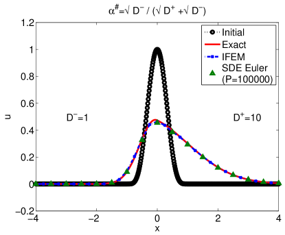
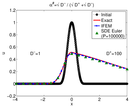
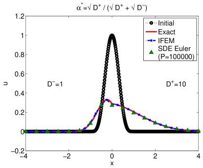
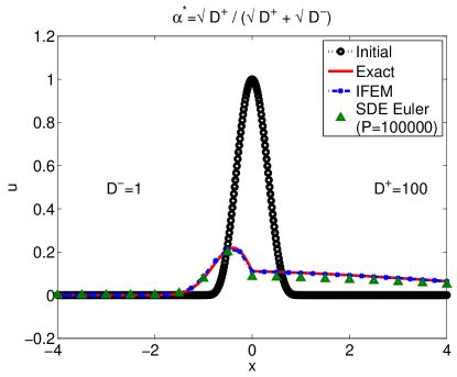
Figure 1: Initial and computed solution of (4.1) at $t=0.2$ using IFEM-CN method, the SDE-Euler method and the expected value solution formula from [4], for various combinations of $D^{+}$ and $\lambda$ values.

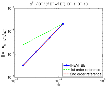
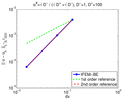
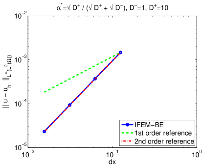
Figure 2: Error for the IFEM-BE method demonstrating second order convergence for the above scenarios.

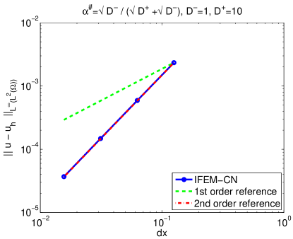
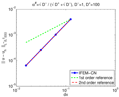
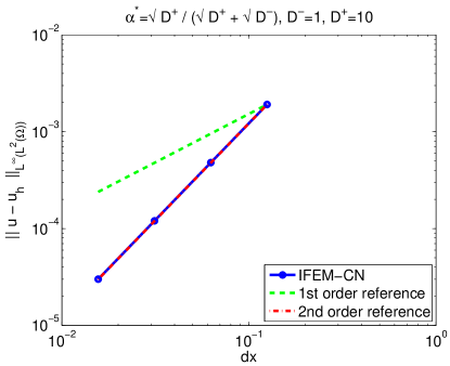
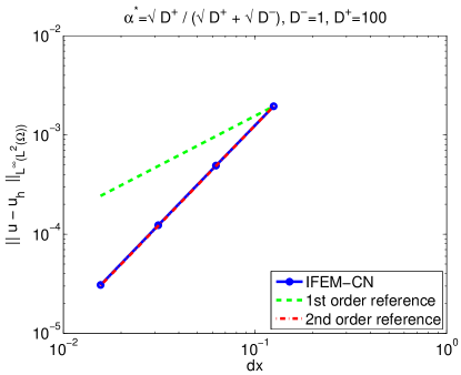
Figure 3: Error for the IFEM-CN method demonstrating second order convergence for the above scenarios.

5 Numerical Methods for Stochastic Diffusion in the Presence of an Interface

In this section we will consider a numerical solution to system (2.1) using a Monte-Carlo method. The discontinuities in the coefficient of the equation, as well as the generality of the interface condition considered in this paper present challenges in two different aspects of the theory. On the one hand, the discontinuity in the diffusion coefficient naturally requires to consider SDE’s that include a local time term (see section 2.1 for details.) As noted in [27], a transformation of the stochastic process can be defined so that this local time term is eliminated. On the other hand, the generality of the interface condition renders inadequate the approach of [27] since they benefited from the self adjoint property of the problem under their consideration. Instead, in the problem consider in this paper, a careful quantification of the effect of the interface condition is needed.

The organization of this section is as follows. In section 5.1 we review basic aspects of Skew Brownian motion, review details of the stochastic representation of solutions of (2.1) obtained in [2], and obtain basic estimates on the corresponding transition probability densities. In section 5.2 we follow a similar approach as the one developed in [27] to eliminate the local time term in the SDE associated to solutions of (2.1), an introduce an Euler-Maruyama method to approximate solutions of the resulting SDE. The main theorems establishing the rate of convergence of the approximation are stated in this section, with proofs given in section 5.3.

5.1 Stochastic Representation of the Solution to (2.1).

Let us first record a definition of skew Brownian motion $B^{(\alpha)}(t)$, $0<\alpha<1$, originally introduced by Itô and McKean. Let $|B(t)|$ denote the reflecting Brownian motion starting at $0$, and enumerate the excursion intervals away from $0$ by $J_{1},J_{2},...$. Let $A_{1},A_{2},...$ be an i.i.d. sequence of Bernoulli $\pm 1$ random variables, independent of $B(t)$, with $P(A_{n}=1)=\alpha$. Then $B^{(\alpha)}(t)$ is defined by changing the signs of the excursion over the intervals $J_{n}$ whenever to $A_{n}=-1$, for $n=1,2,...$. That is

$$B^{(\alpha)}(t)=\sum_{n=1}^{\infty}A_{n}\mathbf{1}_{J_{n}}(t)|B(t)|,\quad t\geq 0.$$ (5.1)

Denote $\sigma(x)=\sqrt{D^{+}}x\mathbf{1}_{[0,\infty)}(x)+\sqrt{D^{-}}x\mathbf{1}_{(-\infty,0)}(x)$ and

$$Y^{(\alpha)}(t)=\sigma\big{(}B^{(\alpha)}(t)\big{)},\quad(t\geq 0).$$ (5.2)

It follows from [2, Theorem 3.1] that if $f\in C^{2}(\mathbb{R}\setminus\{0\})\cap C(\mathbb{R})$ satisfying the condition $\lambda f^{\prime}(0^{+})=(1-\lambda)f^{\prime}(0^{-})$ then, for

$$\alpha=\alpha(\lambda)={\lambda\sqrt{D^{-}}\over\lambda\sqrt{D^{-}}+(1-\lambda)\sqrt{D^{+}}}$$ (5.3)

we have

$$f\big{(}Y^{(\alpha)}(t)\big{)}=f\big{(}Y^{(\alpha)}(0)\big{)}+\int_{0}^{t}f^{\prime}_{-}\big{(}Y^{(\alpha)}(s)\big{)}\sqrt{D\big{(}Y^{(\alpha)}(s)\big{)}}dB(s)+{1\over 2}\int_{0}^{t}D\big{(}Y^{(\alpha)}(s)\big{)}f^{\prime\prime}\big{(}Y^{(\alpha)}(s)\big{)}ds.$$ (5.4)

In addition, $Y^{(\alpha)}(t)$ satisfies the following stochastic differential equation with a local time

$$dY^{(\alpha)}(t)=\sqrt{D\big{(}Y^{(\alpha)}(t)\big{)}}dB(t)+\Big{(}{\sqrt{D^{+}}-\sqrt{D^{-}}\over 2}+\sqrt{D^{-}}{2\alpha-1\over 2\alpha}\Big{)}dl_{t}^{B^{(\alpha)},+}(0)$$ (5.5)

where $D(x)$ is defined as in (2.2) and the local time $l_{t}^{B^{(\alpha)},+}(0)$ is defined by

$$l_{t}^{B^{(\alpha)},+}(0)=\lim_{\epsilon\downarrow 0}{1\over\epsilon}\int_{0}^{t}\mathbf{1}_{[0,\epsilon)}(B^{(\alpha)}(s))d\langle B^{(\alpha)}\rangle_{s}.$$

For each $g\in C^{2}_{b}(\mathbb{R}\setminus\{0\})$ and $x\neq 0$ we denote the operator

$$\tilde{\mathcal{L}}g(x)={D(x)\over 2}g^{\prime\prime}(x).$$ (5.6)

In addition, denote

$$\mathcal{W}^{2} =\{g\in C^{2}_{b}(\mathbb{R}\setminus\{0\}):g^{(i)}\in L^{1}(\mathbb{R})\cap L^{2}(\mathbb{R}),i=1,2;\lambda g^{\prime}(0^{+})=(1-\lambda)g^{\prime}(0^{-})\},$$ (5.7)

$$\mathcal{W}^{4} =\{g\in C^{4}_{b}(\mathbb{R}\setminus\{0\}):g^{(i)}\in L^{1}(\mathbb{R})\cap L^{2}(\mathbb{R}),i=1,...,4;\lambda g^{\prime}(0^{+})=(1-\lambda)g^{\prime}(0^{-}),$$

$$\hskip 223.92305pt\lambda(\tilde{\mathcal{L}}g)^{\prime}(0^{+})=(1-\lambda)(\tilde{\mathcal{L}}g)^{\prime}(0^{-})\}.$$ (5.8)

Now we are in a position to state the stochastic representation theorem which can be found in [2] (see also [27])

Theorem 5.1 (Corollary 3.2 from [2])

Let $0<\lambda<1$, $\alpha=\alpha(\lambda)$ as in (5.3) and $u_{0}\in\mathcal{W}^{2}$. Then the function $u(t,x)=E^{x}u_{0}(Y^{(\alpha)}(t))$, where $(t,x)\in[0,T]\times\mathbb{R}$, is the unique function in $C^{1,2}_{b}([0,T]\times(\mathbb{R}\setminus\{0\}))\cap C([0,T]\times\mathbb{R})$ which satisfies the equations (2.1).

Next, we have some pointwise estimates for the derivatives of $u(t,x)$. A similar result for the case of $\lambda={D^{+}\over D^{+}+D^{-}}$ (continuity of flux) was given in [27].

Theorem 5.2

(i) Let $0<\lambda<1$, $\alpha=\alpha(\lambda)$ as in (5.3). Then the probability distribution of $Y^{(\alpha)}(t)$ under $P^{x}$ (i.e. $Y^{(\alpha)}(0)=x$) has a density $q^{(\alpha)}(t,x,y)$ which satisfies

• There exists $C>0$ such that for all $x\in\mathbb{R}$, $t>0$ and for Lebesgue a.s. $y\in\mathbb{R}\setminus\{0\}$,

  $$q^{(\alpha)}(t,x,y)\leq{C\over\sqrt{t}}.$$ (5.9)

• There exists $C>0$ such that for all $x\in\mathbb{R}$, $t>0$ and $u_{0}\in L^{1}(\mathbb{R})$,

  $$|E^{x}u_{0}\big{(}Y^{(\alpha)}(t)\big{)}|\leq{C\over\sqrt{t}}\|u_{0}\|_{1}.$$ (5.10)

(ii) For all $j=0,1,2$ and $i=1,2,3,4$ satisfying $2j+i\leq 4$ there exists $c>0$ such that for all $x\in\mathbb{R}$, $t>0$ and $u_{0}\in\mathcal{W}^{4}$,

$$\big{|}{\partial^{j}\over\partial t^{j}}{\partial^{i}\over\partial x^{i}}u(t,x)\big{|}\leq{C\over\sqrt{t}}\|u_{0}^{\prime}\|_{\gamma,1},$$ (5.11)

where $\gamma=1$ if $2j+i=1$ or $2$; $\gamma=2$ if $2j+i=3$ or $4$, and $\|g\|_{\gamma,1}=\sum_{i=1}^{\gamma}\|{\partial^{i}g\over\partial x^{i}}\|_{1}$.

The proof of the theorem will be presented in the next subsection to keep the presentation more transparent.

5.2 The Numerical Method

In this section we will construct an explicit one-to-one transformation which transforms $Y^{(\alpha)}$ to a solution to a stochastic differential equation without a local time which can easily be discretized by a standard Euler-Maruyama scheme. Since the transformation is one-to-one and explicit, we can take the inverse transformation of this numerical solution to obtain a numerical approximation for $Y^{(\alpha)}$. As a consequence of Theorem 5.1, we can approximate $u(t,x)$ by $E^{x}u_{0}(Y^{(\alpha)}(t))$ and compute the latter using the Monte-Carlo simulation.

To proceed, we denote

$$\beta(x)=\lambda x\mathbf{1}_{(-\infty,0]}(x)+(1-\lambda)x\mathbf{1}_{(0,\infty)}(x).$$ (5.12)

Then $\beta^{\prime}_{-}(x)=\lambda\mathbf{1}_{(-\infty,0]}(x)+(1-\lambda)\mathbf{1}_{(0,\infty)}(x)$ and $\beta^{-1}(x)={x\over\lambda}\mathbf{1}_{(-\infty,0]}(x)+{x\over 1-\lambda}\mathbf{1}_{(0,\infty)}(x)$. It follows that

$$\theta(x):=\beta_{-}^{\prime}(x)\sqrt{D(x)}=\lambda\sqrt{D^{-}}\mathbf{1}_{(-\infty,0]}(x)+(1-\lambda)\sqrt{D^{+}}\mathbf{1}_{(0,\infty)}(x).$$ (5.13)

Since $\lambda\beta^{\prime}_{-}(0^{+})=(1-\lambda)\beta^{\prime}_{-}(0^{-})$ and $\beta\in C^{2}(\mathbb{R}\setminus\{0\})\cap C(\mathbb{R})$, by virtue of (5.4),

$$\beta\big{(}Y^{(\alpha)}(t)\big{)} =\beta\big{(}Y^{(\alpha)}(0)\big{)}+\int_{0}^{t}\beta^{\prime}_{-}\big{(}Y^{(\alpha)}(s)\big{)}\sqrt{D\big{(}Y^{(\alpha)}(s)\big{)}}dB(s)$$

$$=\beta\big{(}Y^{(\alpha)}(0)\big{)}+\int_{0}^{t}\theta\big{(}\beta\big{(}Y^{(\alpha)}(s)\big{)}\big{)}dB(s).$$ (5.14)

Denote $X(t)=\beta\big{(}Y^{(\alpha)}(t)\big{)}$, then (5.14) yields

$$X(t)=X(0)+\int_{0}^{t}\theta(X(s))dB(s).$$ (5.15)

Let $\Delta=\Delta t={T\over M}$ be the step size. For $0\leq k\leq M$, put $t_{k}=k\Delta t$. Let $\bar{X}^{\Delta}(t)$ be the Euler-Maruyama approximation of $X(t)$,

$$\bar{X}^{\Delta}(t)=\bar{X}^{\Delta}(t_{k})+\theta\big{(}\bar{X}^{\Delta}(t_{k})\big{)}\big{(}B(t)-B(t_{k})\big{)},\quad\bar{X}^{\Delta}(0)=\beta\big{(}Y^{(\alpha)}(0)\big{)}.$$ (5.16)

The numerical solution to (2.1) can be now obtained. Define

$$\bar{Y}^{\Delta}(t)=\beta^{-1}\big{(}\bar{X}^{\Delta}(t)\big{)},\quad u_{\Delta}(T,x)=E^{x}u_{0}(\bar{Y}^{\Delta}(T)).$$ (5.17)

The convergence rate of the above numerical method is given in the following theorem.

Theorem 5.3

For all initial condition $u_{0}\in\mathcal{W}^{4}$, all parameter $0<\epsilon<1/2$ there exists a constant $C$ depending on $\epsilon$ such that for all $n$ large enough, and all $x_{0}\in{\mathbb{R}}$,

$$\big{|}E^{x_{0}}u_{0}(Y^{(\alpha)}(T))-E^{x_{0}}u_{0}(\bar{Y}^{\Delta}(T))\big{|}\leq C\|u_{0}^{\prime}\|_{1,1}\Delta t^{(1-\epsilon)/2}+C\|u_{0}^{\prime}\|_{1,1}\sqrt{\Delta t}+C\|u_{0}^{\prime}\|_{3,1}\Delta t^{1-\epsilon}.$$ (5.18)

Next, we can relax the transmission conditions of $u_{0}$ and $\tilde{\mathcal{L}}u_{0}$ in the above theorem which are required in the definition of $\mathcal{W}_{4}$.

Theorem 5.4

Let $u_{0}:\mathbb{R}\to\mathbb{R}$ be in the space

$$\mathcal{W}=\Big{\{}g\in\mathcal{C}^{4}_{b}(\mathbb{R}\backslash\{0\}),g^{(i)}\in L^{1}(\mathbb{R})\cap L^{2}(\mathbb{R})\text{ for }i=1,...,4\Big{\}}.$$

Then for any parameter $0<\epsilon<1/2$ there exists a constant $C$ depending on $u_{0}$ and $\epsilon$ such that for all $n$ large enough, and all $x_{0}\in{\mathbb{R}}$,

$$\big{|}u_{\Delta}(T,x_{0})-u(T,x_{0})\big{|}\leq C\Delta t^{1/2-\epsilon}.$$ (5.19)

5.3 Proofs

In this section we will gather the proofs of Theorem 5.2, Theorem 5.3 and Theorem 5.4. Proof of Theorem 5.2. The proof will follow from a sequence of steps involving lemmas.

Step $1$: Prove (i).
Let $p^{(\alpha)}(t,x,y)$ be the density function of the skew Brownian motion $B^{(\alpha)}$, then according to [40],

$$p^{(\alpha)}(t,x,y)=\begin{cases}{1\over\sqrt{2\pi t}}e^{-(y-x)^{2}\over 2t}+{(2\alpha-1)\over\sqrt{2\pi t}}e^{-(x+y)^{2}\over 2t},&\text{if $x>0$, $y>0$,}\\ {1\over\sqrt{2\pi t}}e^{-(y-x)^{2}\over 2t}-{(2\alpha-1)\over\sqrt{2\pi t}}e^{-(x+y)^{2}\over 2t},&\text{if $x<0$, $y<0$,}\\ {2\alpha\over\sqrt{2\pi t}}e^{-(y-x)^{2}\over 2t},&\text{if $x\leq 0$, $y>0$,}\\ {2(1-\alpha)\over\sqrt{2\pi t}}e^{-(y-x)^{2}\over 2t},&\text{if $x\geq 0$, $y<0$.}\end{cases}$$ (5.20)

Hence, it follows from (5.2) that $Y^{(\alpha)}(t)$ under $P^{x}$ has a density denoted by $q^{(\alpha)}(t,x,y)$ which satisfies

$$q^{(\alpha)}(t,x,y)={1\over\sqrt{D(y)}}p^{(\alpha)}\Big{(}t,{x\over\sqrt{D(x)}},{y\over\sqrt{D(y)}}\Big{)}.$$ (5.21)

It is clear that (5.20) and (5.21) imply (5.9) and then (5.10).

Step 2: Estimate ${\partial u\over\partial t}(t,x)$. We first prove the following lemma.

Lemma 5.5

There exists a positive constant $C$ such that for all $t\in(0,T]$,

$$\sup_{x\neq 0}\big{|}{\partial u\over\partial t}(t,x)\big{|}\leq{C\over\sqrt{t}}\|u_{0}^{\prime}\|_{1,1}.$$ (5.22)

Proof. Recall that for any $u_{0}\in C^{2}_{b}(\mathbb{R}\setminus\{0\})\cap C(\mathbb{R})$ satisfying $\lambda u_{0}^{\prime}(0^{+})=(1-\lambda)u_{0}^{\prime}(0^{-})$ (5.4) holds true. Hence, for all $x\in\mathbb{R}$ and $t>0$,

$$E^{x}u_{0}\big{(}Y^{(\alpha)}(t)\big{)}=g(x)+\int_{0}^{t}E^{x}\tilde{\mathcal{L}}u_{0}\big{(}Y^{(\alpha)}(s)\big{)}ds,$$ (5.23)

where the operator $\tilde{\mathcal{L}}$ is defined as in (5.6). In addition, notice that

$$dY^{(\alpha)}(t)=\sqrt{\big{(}Y^{(\alpha)}(t)\big{)}}dB(t)+\Big{(}{\sqrt{D^{+}}-\sqrt{D^{-}}\over 2}+\sqrt{D^{-}}{2\alpha-1\over 2\alpha}\Big{)}dl^{B^{(\alpha)},+}_{t}(0).$$ (5.24)

Fix $x>0$. Denote $\tau_{0}(Y^{(\alpha)})=\inf\{s>0:Y^{(\alpha)}(s)=0\}$ and $r_{0}^{x}(s)$ the density of $\tau_{0}(Y^{(\alpha)})\wedge T$ under $P^{x}$. Notice that $\tau_{0}(Y^{(\alpha)})=\tau_{0}\big{(}x+\sqrt{D^{+}}B\big{)}$ where $B(\cdot)$ is the standard Brownian motion. For all function $h$ such that $E^{x}h(Y^{(\alpha)})<\infty$ we have

$$E^{x}h(Y^{(\alpha)}(t))$$

$$=E^{x}\big{[}h(Y^{(\alpha)}(t))\mathbf{1}_{\{\tau_{0}\geq t\}}\big{]}+E^{x}\big{[}h(Y^{(\alpha)}(t))\mathbf{1}_{\{\tau_{0}<t\}}\big{]}$$

$$=E^{x}\big{[}h\big{(}x+\sqrt{D^{+}}B(t)\big{)}\mathbf{1}_{\{\tau_{0}\geq t\}}\big{]}+\int_{0}^{t}E^{0}h\big{(}Y^{(\alpha)}(t-s)\big{)}r_{0}^{x}(s)ds$$

$$=E^{x}h\big{(}x+\sqrt{D^{+}}B(t)\big{)}-E^{x}\big{[}h\big{(}x+\sqrt{D^{+}}B(t)\big{)}\mathbf{1}_{\{\tau_{0}<t\}}\big{]}+\int_{0}^{t}E^{0}h\big{(}Y^{(\alpha)}(t-s)\big{)}r_{0}^{x}(s)ds$$

$$=E^{x}h\big{(}x+\sqrt{D^{+}}B(t)\big{)}-\int_{0}^{t}E^{0}h\big{(}\sqrt{D^{+}}B(s)\big{)}r_{0}^{x}(t-s)ds+\int_{0}^{t}E^{0}h\big{(}Y^{(\alpha)}(s)\big{)}r_{0}^{x}(t-s)ds.$$ (5.25)

For $x<0$ we have a similar identity. To proceed, we assume that $x>0$. From (5.25) we can write

$$u(t,x)=E^{x}u_{0}(Y^{(\alpha)}(t))=E^{x}u_{0}\big{(}x+\sqrt{D^{+}}B(t)\big{)}+v(t,x),$$ (5.26)

where

$$v(t,x) =-\int_{0}^{t}E^{0}u_{0}\big{(}\sqrt{D^{+}}B(s)\big{)}r_{0}^{x}(t-s)ds+\int_{0}^{t}E^{0}u_{0}\big{(}Y^{(\alpha)}(s)\big{)}r_{0}^{x}(t-s)ds$$

$$=\int_{0}^{t}\int_{0}^{t-s}\Big{[}E^{0}\tilde{\mathcal{L}}u_{0}\big{(}Y^{(\alpha)}(\xi)\big{)}-E^{0}\tilde{\mathcal{L}}^{+}u_{0}\big{(}\sqrt{D^{+}}B(\xi)\big{)}\Big{]}d\xi r_{0}^{x}(s)ds$$ (5.27)

and $\tilde{\mathcal{L}}^{+}u_{0}={D^{+}\over 2}u_{0}^{\prime\prime}$. Since

$${\partial v\over\partial t}(t,x)=\int_{0}^{t}\Big{[}E^{0}\tilde{\mathcal{L}}u_{0}\big{(}Y^{(\alpha)}(s)\big{)}-E^{0}\tilde{\mathcal{L}}^{+}u_{0}\big{(}\sqrt{D^{+}}B(s)\big{)}\Big{]}r_{0}^{x}(t-s)ds,$$ (5.28)

according to Lemma 8.1 we obtain,

$$\Big{|}{\partial v\over\partial t}(t,x)\Big{|} \leq\int_{0}^{t}\Big{[}\big{|}E^{0}\tilde{\mathcal{L}}u_{0}\big{(}Y^{(\alpha)}(s)\big{)}\big{|}+\big{|}E^{0}\tilde{\mathcal{L}}^{+}u_{0}\big{(}\sqrt{D^{+}}B(s)\big{)}\big{|}\Big{]}r_{0}^{x}(t-s)ds$$

$$\leq C\big{(}\|\tilde{\mathcal{L}}u_{0}\|_{1}+\|\tilde{\mathcal{L}}^{+}u_{0}\|_{1}\big{)}\int_{0}^{t}{1\over\sqrt{s}}r_{0}^{x}(t-s)ds$$

$$\leq{C\over\sqrt{t}}\big{(}\|\tilde{\mathcal{L}}u_{0}\|_{1}+\|\tilde{\mathcal{L}}^{+}u_{0}\|_{1}\big{)}.$$ (5.29)

Next we estimate ${\partial\over\partial t}E^{x}u_{0}(x+\sqrt{D^{+}}B(t))$. It is obvious that the density $q^{+}(t,x,y)$ of $x+\sqrt{D^{+}}B(t)$ satisfies the inequality $q^{+}(t,x,y)\leq{C\over\sqrt{t}}\exp\{-{(y-x)^{2}\over\nu t}\}$ for all $0\leq t\leq T$ for some constants $C,\nu$. It follows from the equation

$${\partial\over\partial t}E^{x}u_{0}(x+\sqrt{D^{+}}B(t))=E^{x}\tilde{\mathcal{L}}^{+}\big{(}u_{0}(x+\sqrt{D^{+}}B(t))\big{)}={D^{+}\over 2}\int u_{0}^{\prime\prime}(y)q^{+}(t,x,y)dy$$

that

$$\sup_{x\in\mathbb{R}}\Big{|}{\partial\over\partial t}E^{x}u_{0}(x+\sqrt{D^{+}}B(t))\Big{|}\leq{C\over\sqrt{t}}\|\tilde{\mathcal{L}}^{+}u_{0}\|_{1}$$ (5.30)

Combining (5.26), (5.29) and (5.30) we derive (5.22) as desired.$\qquad\Box$

Lemma 5.6

There exists a positive constant $C$ such that for all $t\in(0,T]$,

$$\sup_{x\neq 0}\big{|}{\partial^{2}u\over\partial t^{2}}(t,x)\big{|}\leq{C\over\sqrt{t}}\|u_{0}^{\prime}\|_{3,1}.$$ (5.31)

Proof. For $u_{0}\in\mathcal{W}^{4}$, $\tilde{\mathcal{L}}u_{0}\in\mathcal{W}^{2}$. By virtue of (5.26) and (5.28) we have

$${\partial^{2}u\over\partial t^{2}}(t,x) ={\partial^{2}\over\partial t^{2}}E^{x}u_{0}(x+\sqrt{D^{+}}B(t))$$

$$\quad+\int_{0}^{t}{\partial\over\partial t}\Big{[}E^{0}\tilde{\mathcal{L}}u_{0}\big{(}Y^{(\alpha)}(t-s)\big{)}-E^{0}\tilde{\mathcal{L}}^{+}u_{0}\big{(}\sqrt{D^{+}}B(t-s)\big{)}\Big{]}r_{0}^{x}(s)ds$$

$$={\partial\over\partial t}E^{x}\tilde{\mathcal{L}}^{+}u_{0}(x+\sqrt{D^{+}}B(t))$$

$$\quad+\int_{0}^{t}\Big{[}E^{0}\tilde{\mathcal{L}}(\tilde{\mathcal{L}}u_{0})\big{(}Y^{(\alpha)}(s)\big{)}-E^{0}\tilde{\mathcal{L}}^{+}(\tilde{\mathcal{L}}^{+}u_{0})\big{(}\sqrt{D^{+}}B(s)\big{)}\Big{]}r_{0}^{x}(t-s)ds.$$

Therefore, by Lemma 5.5, we obtain

$$\Big{|}{\partial^{2}u\over\partial t^{2}}(t,x)\Big{|}\leq{C\over\sqrt{t}}\|\tilde{\mathcal{L}}^{+}(\tilde{\mathcal{L}}^{+}u_{0})\|_{1}+{C\over\sqrt{t}}\Big{(}\|\tilde{\mathcal{L}}(\tilde{\mathcal{L}}u_{0})\|_{1}+\|\tilde{\mathcal{L}}^{+}(\tilde{\mathcal{L}}^{+}u_{0})\|_{1}\Big{)}={C\over\sqrt{t}}\|u_{0}^{\prime}\|_{3,1}.$$ (5.32)

Step 3: Estimate ${\partial^{i}u\over\partial x^{i}}(t,x)$. We have the following lemma.

Lemma 5.7

There exists a positive constant $C$ such that for all $t\in(0,T]$,

$$\sup_{x\neq 0}\big{|}{\partial u\over\partial x}(t,x)\big{|}\leq{C\over\sqrt{t}}\|u_{0}^{\prime}\|_{1,1}.$$ (5.33)

Proof. Since ${\partial\over\partial x}E^{x}u_{0}(x+\sqrt{D^{+}}B(t))=E^{x}u_{0}^{\prime}(x+\sqrt{D^{+}}B(t))$, we have

$$\Big{\|}{\partial\over\partial x}E^{x}u_{0}(x+\sqrt{D^{+}}B(t))\Big{\|}_{\infty} =\big{\|}E^{x}u_{0}^{\prime}(x+\sqrt{D^{+}}B(t))\big{\|}_{\infty}$$

$$=\big{\|}\int u_{0}^{\prime}(y)q^{+}(t,x,y)dy\big{\|}_{\infty}$$

$$\leq{C\over\sqrt{t}}\big{\|}\int u_{0}^{\prime}(y)e^{-{(y-x)^{2}\over D^{+}t^{2}}}dy\big{\|}_{\infty}\leq{C\over\sqrt{t}}\|u_{0}^{\prime}\|_{1}.$$ (5.34)

Let $H(s)=\int_{0}^{s}\big{[}E^{0}\tilde{\mathcal{L}}u_{0}(Y^{(\alpha)}(\xi))-E^{0}\tilde{\mathcal{L}}^{+}u_{0}(x+\sqrt{D^{+}}B(\xi))\big{]}d\xi$, then since $H(0)=0$ and $H^{\prime}(s)\leq C\big{(}\|\tilde{\mathcal{L}}u_{0}\|_{1}+\|\tilde{\mathcal{L}}^{+}u_{0}\|_{1}\big{)}={C_{H}\over s^{0}}$ we have by (5.27) and Lemma 8.2 that

$$v(t,x)=\int_{0}^{t}H(s)r_{0}^{x}(t-s)ds$$

and

$$\Big{|}{\partial v\over\partial x}(t,x)\Big{|}\leq\tilde{C}\big{(}\|\tilde{\mathcal{L}}^{+}u_{0}\|_{1}+\|\tilde{\mathcal{L}}u_{0}\|_{1}\big{)}.$$ (5.35)

In view of (5.26), (5.34) and (5.35) we obtain (5.33).$\qquad\Box$

By the similar way we can prove the estimates for $|{\partial^{j}\over\partial t^{j}}{\partial^{i}\over\partial x^{i}}u(t,x)|$ for $2j+i\leq 4$.$\qquad\Box$

Proof of Theorem 5.3. Denote $s_{k}=T-t_{k}$ for $0\leq k\leq M$. Since $u(0,x)=u_{0}(x)$ and $u(T,x)=E^{x}u_{0}(Y^{(\alpha)}(T))$,

$$u(0,\beta^{-1}(\bar{X}^{\Delta}(T))=u_{0}(\beta^{-1}(\bar{X}^{\Delta}(T))),$$

$$u(T,x_{0})=u(T,\bar{X}^{\Delta}(0))=u(T,\beta^{-1}(Y^{(\alpha)}(0))=E^{x_{0}}u_{0}(Y^{(\alpha)}(T)).$$

Therefore,

$$\epsilon_{T}^{x_{0}} =\Big{|}E^{x_{0}}u_{0}\big{(}Y^{(\alpha)}(T)\big{)}-E^{x_{0}}u_{0}\big{(}\bar{Y}^{\Delta}(T)\big{)}\Big{|}=\Big{|}E^{x_{0}}u_{0}\big{(}\beta^{-1}(\bar{X}(T))\big{)}-E^{x_{0}}u_{0}\big{(}\beta^{-1}(\bar{X}^{\Delta}(T))\big{)}\Big{|}$$

$$=\Big{|}E^{x_{0}}u\big{(}T,\beta^{-1}(\bar{X}^{\Delta}(0))\big{)}-E^{x_{0}}u\big{(}0,\beta^{-1}(\bar{X}^{\Delta}(T))\big{)}\Big{|}$$

$$=\Big{|}\sum_{k=0}^{M-1}\Big{[}E^{x_{0}}u\big{(}T-t_{k},\beta^{-1}(\bar{X}^{\Delta}(t_{k}))\big{)}-E^{x_{0}}u\big{(}T-t_{k+1},\beta^{-1}(\bar{X}^{\Delta}(t_{k+1}))\big{)}\Big{]}\Big{|}$$

$$\leq\Big{|}\sum_{k=0}^{M-2}\Big{[}E^{x_{0}}u\big{(}s_{k},\beta^{-1}(\bar{X}^{\Delta}(t_{k}))\big{)}-E^{x_{0}}u\big{(}s_{k+1},\beta^{-1}(\bar{X}^{\Delta}(t_{k+1}))\big{)}\Big{]}\Big{|}$$

$$\quad+\Big{|}E^{x_{0}}u\big{(}s_{M-1},\beta^{-1}(\bar{X}^{\Delta}(t_{M-1}))\big{)}-E^{x_{0}}u\big{(}0,\beta^{-1}(\bar{X}^{\Delta}(T))\big{)}\Big{|}.$$ (5.36)

To estimate the second term in (5.36), we use the fact that $u(0,x)=u_{0}(x)$ and obtain

$$\Big{|}E^{x_{0}}u\big{(}s_{M-1},\beta^{-1}(\bar{X}^{\Delta}(t_{M-1}))\big{)}-E^{x_{0}}u\big{(}0,\beta^{-1}(\bar{X}^{\Delta}(T))\big{)}\Big{|}$$

$$\quad\leq\Big{|}E^{x_{0}}u\big{(}s_{M-1},\beta^{-1}(\bar{X}^{\Delta}(t_{M-1}))\big{)}-E^{x_{0}}u\big{(}0,\beta^{-1}(\bar{X}^{\Delta}(t_{M-1}))\big{)}\Big{|}$$

$$\quad\quad+\Big{|}E^{x_{0}}u_{0}\big{(}\beta^{-1}(\bar{X}^{\Delta}(t_{M-1}))\big{)}-E^{x_{0}}u_{0}\big{(}\beta^{-1}(\bar{X}^{\Delta}(T))\big{)}\Big{|}.$$

Since $u_{0}^{\prime\prime}$ is in $L_{1}({\mathbb{R}})$, $u_{0}^{\prime}$ is bounded and $u_{0}\circ\beta^{-1}$ is Lipschitz. By virtue of the inequality $\sup_{x\neq 0}|{\partial u\over\partial t}(t,x)|\leq{C\over\sqrt{t}}\|u_{0}^{\prime}\|_{1,1}$ we have

$$\Big{|}E^{x_{0}}u\big{(}s_{M-1},\beta^{-1}(\bar{X}^{\Delta}(t_{M-1}))\big{)}-E^{x_{0}}u\big{(}0,\beta^{-1}(\bar{X}^{\Delta}(T))\big{)}\Big{|}\leq C\|u_{0}^{\prime}\|_{1,1}\sqrt{\Delta t}.$$ (5.37)

It remains to estimate the first term in (5.36). To proceed, we denote the time and space increments as follow

$$T_{k} =u\big{(}s_{k},\beta^{-1}(\bar{X}^{\Delta}(t_{k}))\big{)}-u\big{(}s_{k+1},\beta^{-1}(\bar{X}^{\Delta}(t_{k}))\big{)},$$

$$S_{k} =u\big{(}s_{k+1},\beta^{-1}(\bar{X}^{\Delta}(t_{k+1}))\big{)}-u\big{(}s_{k+1},\beta^{-1}(\bar{X}^{\Delta}(t_{k}))\big{)}.$$

The first term in (5.36) then can be rewritten as $\big{|}\sum_{k=0}^{M-2}E^{x_{0}}(T_{k}-S_{k})\big{|}$. The analysis of this term will be divided into $4$ steps.

Step 1: Estimate for the time increment $T_{k}$: Since $s_{k}-s_{k+1}=\Delta t$, by the definition of $T_{k}$ and Taylor expansion we have

$$\Big{[}u\big{(}s_{k},\beta^{-1}(\bar{X}^{\Delta}(t_{k}))\big{)}-u\big{(}s_{k+1},\beta^{-1}(\bar{X}^{\Delta}(t_{k}))\big{)}\Big{]}1_{\{\bar{X}^{\Delta}(t_{k})>0\}}$$

$$=\Delta t{\partial u\over\partial t}\big{(}s_{k+1},\beta^{-1}(\bar{X}^{\Delta}(t_{k}))\big{)}1_{\{\bar{X}^{\Delta}(t_{k})>0\}}$$

$$\quad+\Delta t^{2}\int_{[0,1]^{2}}{\partial^{2}u\over\partial t^{2}}\big{(}s_{k+1}+\tau_{1}\tau_{2}\Delta t,\beta^{-1}(\bar{X}^{\Delta}(t_{k}))\big{)}\tau_{1}d\tau_{1}d\tau_{2}1_{\{\bar{X}^{\Delta}(t_{k})>0\}}$$

$$=T^{+}_{k}+R^{+}_{k}.$$

Similarly,

$$\Big{[}u\big{(}s_{k},\beta^{-1}(\bar{X}^{\Delta}(t_{k}))\big{)}-u\big{(}s_{k+1},\beta^{-1}(\bar{X}^{\Delta}(t_{k}))\big{)}\Big{]}1_{\{\bar{X}^{\Delta}(t_{k})<0\}}$$

$$=\Delta t{\partial u\over\partial t}\big{(}s_{k+1},\beta^{-1}(\bar{X}^{\Delta}(t_{k}))\big{)}1_{\{\bar{X}^{\Delta}(t_{k})<0\}}$$

$$\quad+\Delta t^{2}\int_{[0,1]^{2}}{\partial^{2}u\over\partial t^{2}}\big{(}s_{k+1}+\tau_{1}\tau_{2}\Delta t,\beta^{-1}(\bar{X}^{\Delta}(t_{k}))\big{)}\tau_{1}d\tau_{1}d\tau_{2}1_{\{\bar{X}^{\Delta}(t_{k})<0\}}$$

$$=T^{-}_{k}+R^{-}_{k}.$$

It follows from the above equations and the inequality $\sup_{x\neq 0}|{\partial^{2}u\over\partial t^{2}}(t,x)|\leq{C\over\sqrt{t}}\|u_{0}^{\prime}\|_{3,1}$ that

$$E^{x_{0}}\big{|}R^{+}_{k}+R^{-}_{k}\big{|}=E^{x_{0}}\Delta t^{2}\Big{|}\int_{[0,1]^{2}}{\partial^{2}u\over\partial t^{2}}\big{(}s_{k+1}+\tau_{1}\tau_{2}\Delta t,\beta^{-1}(\bar{X}^{\Delta}(t_{k}))\big{)}\tau_{1}d\tau_{1}d\tau_{2}\Big{|}\leq{C\Delta t^{2}\over\sqrt{s_{k+1}}}\|u_{0}^{\prime}\|_{3,1}.$$

Therefore, we obtain

$$E^{x_{0}}T_{k}=\Delta tE^{x_{0}}\Big{[}{\partial u\over\partial t}\big{(}s_{k+1},\beta^{-1}(\bar{X}^{\Delta}(t_{k}))\big{)}\Big{]}+O\left({\Delta t^{2}\over\sqrt{s_{k+1}}}\right).$$ (5.38)

Step 2: Estimate for the space increment $S_{k}$: Let us denote the following increments

$$\triangle_{k+1}B =B(t_{k+1})-B(t_{k}),$$

$$\triangle_{k+1}\bar{X}^{\Delta} =\theta\big{(}\bar{X}^{\Delta}(t_{k})\big{)}\triangle_{k+1}B,$$

$$\tilde{\triangle}_{k+1}\bar{Y}^{\Delta} ={\triangle_{k+1}\bar{X}^{\Delta}\over 1-\lambda}1_{\{\bar{X}^{\Delta}(t_{k})>0\}}+{\triangle_{k+1}\bar{X}^{\Delta}\over\lambda}1_{\{\bar{X}^{\Delta}(t_{k})<0\}},$$ (5.39)

and events

$$\Omega_{k}^{++} =\big{\{}\bar{X}^{\Delta}(t_{k})>0,\bar{X}^{\Delta}(t_{k+1})>0\big{\}},\quad\Omega_{k}^{+-}=\big{\{}\bar{X}^{\Delta}(t_{k})>0,\bar{X}^{\Delta}(t_{k+1})\leq 0\big{\}},$$

$$\Omega_{k}^{--} =\big{\{}\bar{X}^{\Delta}(t_{k})\leq 0,\bar{X}^{\Delta}(t_{k+1})\leq 0\big{\}},\quad\Omega_{k}^{-+}=\big{\{}\bar{X}^{\Delta}(t_{k})\leq 0,\bar{X}^{\Delta}(t_{k+1})>0\big{\}}.$$

Hence, by the definition of the function $\beta$, on $\Omega^{++}_{k}$,

$$\beta^{-1}\big{(}\bar{X}^{\Delta}(t_{k+1})\big{)}=\beta^{-1}\big{(}\bar{X}^{\Delta}(t_{k})\big{)}+{\triangle_{k+1}\bar{X}^{\Delta}\over 1-\lambda}.$$

This and Taylor expansion yield

$$S_{k}1_{\Omega^{++}_{k}}$$

$$={\triangle_{k+1}\bar{X}^{\Delta}\over 1-\lambda}{\partial u\over\partial x}\big{(}s_{k+1},\beta^{-1}(\bar{X}^{\Delta}(t_{k}))\big{)}1_{\Omega^{++}_{k}}+{1\over 2}{(\triangle_{k+1}\bar{X}^{\Delta})^{2}\over(1-\lambda)^{2}}{\partial^{2}u\over\partial x^{2}}\big{(}s_{k+1},\beta^{-1}(\bar{X}^{\Delta}(t_{k}))\big{)}1_{\Omega^{++}_{k}}$$

$$\quad+{1\over 6}{(\triangle_{k+1}\bar{X}^{\Delta})^{3}\over(1-\lambda)^{3}}{\partial^{3}u\over\partial x^{3}}\big{(}s_{k+1},\beta^{-1}(\bar{X}^{\Delta}(t_{k}))\big{)}1_{\Omega^{++}_{k}}$$

$$\quad+{(\triangle_{k+1}\bar{X}^{\Delta})^{4}\over(1-\lambda)^{4}}\int_{[0,1]^{4}}{\partial^{4}u\over\partial x^{4}}\Big{(}s_{k+1},\beta^{-1}(\bar{X}^{\Delta}(t_{k}))+\tau_{1}\tau_{2}\tau_{3}\tau_{4}{\triangle_{k+1}\bar{X}^{\Delta}\over 1-\lambda}\Big{)}\tau_{1}\tau_{2}\tau_{3}d\tau_{1}...d\tau_{4}1_{\Omega^{++}_{k}}$$

$$=:S_{k}^{++1}+S_{k}^{++2}+S_{k}^{++3}+S_{k}^{++4}.$$

Similarly,

$$S_{k}1_{\Omega^{--}_{k}}$$

$$={\triangle_{k+1}\bar{X}^{\Delta}\over\lambda}{\partial u\over\partial x}\big{(}s_{k+1},\beta^{-1}(\bar{X}^{\Delta}(t_{k}))\big{)}1_{\Omega^{--}_{k}}+{1\over 2}{(\triangle_{k+1}\bar{X}^{\Delta})^{2}\over\lambda^{2}}{\partial^{2}u\over\partial x^{2}}\big{(}s_{k+1},\beta^{-1}(\bar{X}^{\Delta}(t_{k}))\big{)}1_{\Omega^{--}_{k}}$$

$$\quad+{1\over 6}{(\triangle_{k+1}\bar{X}^{\Delta})^{3}\over\lambda^{3}}{\partial^{3}u\over\partial x^{3}}\big{(}s_{k+1},\beta^{-1}(\bar{X}^{\Delta}(t_{k}))\big{)}1_{\Omega^{--}_{k}}$$

$$\quad+{(\triangle_{k+1}\bar{X}^{\Delta})^{4}\over\lambda^{4}}\int_{[0,1]^{4}}{\partial^{4}u\over\partial x^{4}}\Big{(}s_{k+1},\beta^{-1}(\bar{X}^{\Delta}(t_{k}))+\tau_{1}\tau_{2}\tau_{3}\tau_{4}{\triangle_{k+1}\bar{X}^{\Delta}\over\lambda}\Big{)}\tau_{1}\tau_{2}\tau_{3}d\tau_{1}...d\tau_{4}1_{\Omega^{--}_{k}}$$

$$=:S_{k}^{--1}+S_{k}^{--2}+S_{k}^{--3}+S_{k}^{--4}.$$

Since $\Omega^{++}_{k}\cup\Omega^{--}_{k}=\Omega-(\Omega^{+-}_{k}\cup\Omega^{-+}_{k})$ and $\Omega^{+-}_{k}\cup\Omega^{-+}_{k}\in\sigma\{B(t):0\leq t\leq t_{k+1}\}$, by (5.39) we get

$$E^{x_{0}}(S^{++1}_{k}+S^{--1}_{k})$$

$$=E^{x_{0}}\Big{[}{\triangle_{k+1}\bar{X}^{\Delta}\over 1-\lambda}{\partial u\over\partial x}\big{(}s_{k+1},\beta^{-1}(\bar{X}^{\Delta}(t_{k}))\big{)}1_{\Omega^{++}_{k}}+{\triangle_{k+1}\bar{X}^{\Delta}\over\lambda}{\partial u\over\partial x}\big{(}s_{k+1},\beta^{-1}(\bar{X}^{\Delta}(t_{k}))\big{)}1_{\Omega^{--}_{k}}\Big{]}$$

$$\quad+E^{x_{0}}\big{[}\tilde{\triangle}_{k+1}\bar{Y}^{\Delta}{\partial u\over\partial x}\big{(}s_{k+1},\beta^{-1}(\bar{X}^{\Delta}(t_{k}))\big{)}1_{\{\Omega^{+-}_{k}\cup\Omega^{-+}_{k}\}}\big{]}$$

$$\quad-E^{x_{0}}\big{[}\tilde{\triangle}_{k+1}\bar{Y}^{\Delta}{\partial u\over\partial x}\big{(}s_{k+1},\beta^{-1}(\bar{X}^{\Delta}(t_{k}))\big{)}1_{\{\Omega^{+-}_{k}\cup\Omega^{-+}_{k}\}}\big{]}$$

$$=E^{x_{0}}\Big{[}\Big{(}{\triangle_{k+1}\bar{X}^{\Delta}\over 1-\lambda}1_{\{\bar{X}^{\Delta}(t_{k})>0\}}+{\triangle_{k+1}\bar{X}^{\Delta}\over\lambda}1_{\{\bar{X}^{\Delta}(t_{k})<0\}}\Big{)}{\partial u\over\partial x}\big{(}s_{k+1},\beta^{-1}(\bar{X}^{\Delta}(t_{k}))\big{)}\Big{]}$$

$$\quad-E^{x_{0}}\big{[}\tilde{\triangle}_{k+1}\bar{Y}^{\Delta}{\partial u\over\partial x}\big{(}s_{k+1},\beta^{-1}(\bar{X}^{\Delta}(t_{k}))\big{)}1_{\{\Omega^{+-}_{k}\cup\Omega^{-+}_{k}\}}\big{]}$$

$$=-E^{x_{0}}\big{[}\tilde{\triangle}_{k+1}\bar{Y}^{\Delta}{\partial u\over\partial x}\big{(}s_{k+1},\beta^{-1}(\bar{X}^{\Delta}(t_{k}))\big{)}1_{\{\Omega^{+-}_{k}\cup\Omega^{-+}_{k}\}}\big{]}.$$

By the similar way and notice that $E\big{(}(\triangle_{k+1}B)^{2}\big{|}\,B(t),\,0\leq t\leq t_{k}\big{)}=\Delta t$, we obtain

$$E^{x_{0}}(S^{++2}_{k}+S^{--2}_{k})$$

$$={1\over 2}E^{x_{0}}\Big{\{}\Big{[}\Big{(}{\triangle_{k+1}\bar{X}^{\Delta}\over 1-\lambda}\Big{)}^{2}1_{\Omega^{++}_{k}}+\Big{(}{\triangle_{k+1}\bar{X}^{\Delta}\over\lambda}\Big{)}^{2}1_{\Omega^{--}_{k}}\Big{]}{\partial^{2}u\over\partial x^{2}}\big{(}s_{k+1},\beta^{-1}(\bar{X}^{\Delta}(t_{k}))\big{)}\Big{\}}$$

$$={1\over 2}E^{x_{0}}\Big{\{}\Big{[}\Big{(}{\theta(\bar{X}^{\Delta}(t_{k}))\triangle_{k+1}B\over 1-\lambda}\Big{)}^{2}1_{\{\bar{X}^{\Delta}(t_{k})>0\}}+\Big{(}{\theta(\bar{X}^{\Delta}(t_{k}))\triangle_{k+1}B\over\lambda}\Big{)}^{2}1_{\{\bar{X}^{\Delta}(t_{k})<0\}}\Big{]}$$

$$\quad\times{\partial^{2}u\over\partial x^{2}}\big{(}s_{k+1},\beta^{-1}(\bar{X}^{\Delta}(t_{k}))\big{)}\Big{\}}-{1\over 2}E^{x_{0}}\big{[}\big{(}\tilde{\triangle}_{k+1}\bar{Y}^{\Delta}\big{)}^{2}{\partial^{2}u\over\partial x^{2}}\big{(}s_{k+1},\beta^{-1}(\bar{X}^{\Delta}(t_{k}))\big{)}1_{\{\Omega^{+-}_{k}\cup\Omega^{-+}_{k}\}}\big{]}$$

$$={\Delta t\over 2}E^{x_{0}}\Big{\{}\Big{[}D^{+}1_{\{\bar{X}^{\Delta}(t_{k})>0\}}+D^{-}1_{\{\bar{X}^{\Delta}(t_{k})<0\}}\Big{]}{\partial^{2}u\over\partial x^{2}}\big{(}s_{k+1},\beta^{-1}(\bar{X}^{\Delta}(t_{k}))\big{)}\Big{\}}$$

$$\quad-{1\over 2}E^{x_{0}}\big{[}\big{(}\tilde{\triangle}_{k+1}\bar{Y}^{\Delta}\big{)}^{2}{\partial^{2}u\over\partial x^{2}}\big{(}s_{k+1},\beta^{-1}(\bar{X}^{\Delta}(t_{k}))\big{)}1_{\{\Omega^{+-}_{k}\cup\Omega^{-+}_{k}\}}\big{]}$$

$$={\Delta t\over 2}E^{x_{0}}\Big{[}D\big{(}\beta^{-1}(\bar{X}^{\Delta}(t_{k}))\big{)}{\partial^{2}u\over\partial x^{2}}\big{(}s_{k+1},\beta^{-1}(\bar{X}^{\Delta}(t_{k}))\big{)}\Big{]}$$

$$\quad-{1\over 2}E^{x_{0}}\big{[}\big{(}\tilde{\triangle}_{k+1}\bar{Y}^{\Delta}\big{)}^{2}{\partial^{2}u\over\partial x^{2}}\big{(}s_{k+1},\beta^{-1}(\bar{X}^{\Delta}(t_{k}))\big{)}1_{\{\Omega^{+-}_{k}\cup\Omega^{-+}_{k}\}}\big{]}.$$

Since $E\big{(}(\triangle_{k+1}B)^{3}\big{|}\,B(t),\,0\leq t\leq t_{k}\big{)}=0$,

$$E^{x_{0}}(S^{++3}_{k}+S^{--3}_{k})=-{1\over 6}E^{x_{0}}\big{[}\big{(}\tilde{\triangle}_{k+1}\bar{Y}^{\Delta}\big{)}^{3}{\partial^{3}u\over\partial x^{3}}\big{(}s_{k+1},\beta^{-1}(\bar{X}^{\Delta}(t_{k}))\big{)}1_{\{\Omega^{+-}_{k}\cup\Omega^{-+}_{k}\}}\big{]}.$$

Next, according to Theorem 2,

$$E^{x_{0}}\big{|}S^{++4}_{k}+S^{--4}_{k}\big{|}\leq{C\Delta t^{2}\over\sqrt{s_{k+1}}}\|u_{0}^{\prime}\|_{3,1}.$$

Combining the calculations above, we arrive at

$$E^{x_{0}}S_{k} =E^{x_{0}}\tilde{\mathcal{L}}u\big{(}s_{k+1},\beta^{-1}(\bar{X}^{\Delta}(t_{k}))\big{)}\Delta t$$

$$\quad\quad+E^{x_{0}}\Big{\{}\Big{[}S_{k}-\tilde{\triangle}_{k+1}\bar{Y}^{\Delta}{\partial u\over\partial x}\big{(}s_{k+1},\beta^{-1}(\bar{X}^{\Delta}(t_{k}))\big{)}\Big{]}1_{\{\Omega^{+-}_{k}\cup\Omega^{-+}_{k}\}}$$

$$\quad\quad-{1\over 2}\big{(}\tilde{\triangle}_{k+1}\bar{Y}^{\Delta}\big{)}^{2}{\partial^{2}u\over\partial x^{2}}\big{(}s_{k+1},\beta^{-1}(\bar{X}^{\Delta}(t_{k}))\big{)}1_{\{\Omega^{+-}_{k}\cup\Omega^{-+}_{k}\}}$$

$$\quad\quad-{1\over 6}\big{(}\tilde{\triangle}_{k+1}\bar{Y}^{\Delta}\big{)}^{3}{\partial^{3}u\over\partial x^{3}}\big{(}s_{k+1},\beta^{-1}(\bar{X}^{\Delta}(t_{k}))\big{)}1_{\{\Omega^{+-}_{k}\cup\Omega^{-+}_{k}\}}\Big{\}}+O\Big{(}{\Delta t^{2}\over\sqrt{s_{k+1}}}\Big{)}$$

$$=:E^{x_{0}}\tilde{\mathcal{L}}u\big{(}s_{k+1},\beta^{-1}(\bar{X}^{\Delta}(t_{k}))\big{)}\Delta t+E^{x_{0}}\mathcal{R}_{k}+O\Big{(}{\Delta t^{2}\over\sqrt{s_{k+1}}}\Big{)}.$$ (5.40)

We now estimate the remaining term $E^{x_{0}}\mathcal{R}_{k}$.

Step 3: Estimate $E^{x_{0}}\mathcal{R}_{k}$:

For any fixed $\epsilon\in(0,1/2)$, we will show that

$$|E^{x_{0}}\mathcal{R}_{k}| \leq{C\Delta t^{1-2\epsilon}\over\sqrt{s_{k+1}}}\|u_{0}^{\prime}\|_{1,1}P^{x_{0}}\Big{\{}\big{|}\bar{X}^{\Delta}(t_{k})\big{|}\leq\Delta t^{{1\over 2}-\epsilon}\Big{\}}$$

$$\quad\quad\quad+{C\Delta t^{{3\over 2}-3\epsilon}\over\sqrt{s_{k+1}}}\|u_{0}^{\prime}\|_{3,1}P^{x_{0}}\Big{\{}\big{|}\bar{X}^{\Delta}(t_{k})\big{|}\leq\Delta t^{{1\over 2}-\epsilon}\Big{\}}.$$ (5.41)

Notice that we can rewrite $\Omega^{+-}_{k}$ as

$$\Omega^{+-}_{k}= \,\,\Big{\{}\bar{X}^{\Delta}(t_{k})\geq\Delta t^{{1\over 2}-\epsilon},\,\,\bar{X}^{\Delta}(t_{k+1})\leq 0\Big{\}}\cup\Big{\{}0<\bar{X}^{\Delta}(t_{k})\leq\Delta t^{{1\over 2}-\epsilon},\,\,\bar{X}^{\Delta}(t_{k+1})\leq-\Delta t^{{1\over 2}-\epsilon}\Big{\}}$$

$$\cup\Big{\{}0<\bar{X}^{\Delta}(t_{k})\leq\Delta t^{{1\over 2}-\epsilon},\,\,-\Delta t^{{1\over 2}-\epsilon}\leq\bar{X}^{\Delta}(t_{k+1})\leq 0\Big{\}}.$$

Since $\bar{X}^{\Delta}(t_{k+1})=\bar{X}^{\Delta}(t_{k})+\theta\big{(}\bar{X}^{\Delta}(t_{k})\big{)}B(\Delta t)$, it follows that

$$P\Big{\{}\bar{X}^{\Delta}(t_{k})\geq\Delta t^{{1\over 2}-\epsilon},\,\,\bar{X}^{\Delta}(t_{k+1})\leq 0\Big{\}}\leq P\Big{\{}(1-\lambda)\sqrt{D^{+}}B(\Delta t)\geq\Delta t^{{1\over 2}-\epsilon}\Big{\}}\leq C\exp\{-CM^{\epsilon}\}.$$

Similarly,

$$P\Big{\{}0<\bar{X}^{\Delta}(t_{k})\leq\Delta t^{{1\over 2}-\epsilon},\,\,\bar{X}^{\Delta}(t_{k+1})\leq-\Delta t^{{1\over 2}-\epsilon}\Big{\}}\leq C\exp\{-CM^{\epsilon}\}.$$

We can proceed analogously on the event $\Omega^{-+}_{k}$. This leads us to limit to consider the events

$$\hat{\Omega}^{+-}_{k} =\Big{\{}0<\bar{X}^{\Delta}(t_{k})\leq\Delta t^{{1\over 2}-\epsilon},\,\,-\Delta t^{{1\over 2}-\epsilon}\leq\bar{X}^{\Delta}(t_{k+1})\leq 0\Big{\}},$$

$$\hat{\Omega}^{-+}_{k} =\Big{\{}-\Delta t^{{1\over 2}-\epsilon}\leq\bar{X}^{\Delta}(t_{k})<0,\,\,0\leq\bar{X}^{\Delta}(t_{k+1})\leq\Delta t^{{1\over 2}-\epsilon}\Big{\}}.$$

Note that, by (5.39), $\tilde{\triangle}_{k+1}\bar{Y}^{\Delta}\leq C\Delta t^{1/2-\epsilon}$ on these sets. Hence, we have

$$\Big{|}E^{x_{0}}\Big{[}\big{(}\tilde{\triangle}_{k+1}\bar{Y}^{\Delta}\big{)}^{2}{\partial^{2}u\over\partial x^{2}}\big{(}s_{k+1},\beta^{-1}(\bar{X}^{\Delta}(t_{k}))\big{)}1_{\{\hat{\Omega}^{+-}_{k}\cup\hat{\Omega}^{-+}_{k}\}}\Big{]}\Big{|}$$

$$\quad\leq{C\Delta t^{1-2\epsilon}\over\sqrt{s_{k+1}}}\|u_{0}^{\prime}\|_{1,1}P^{x_{0}}\Big{\{}\big{|}\bar{X}^{\Delta}(t_{k})\big{|}\leq\Delta t^{{1\over 2}-\epsilon}\Big{\}},$$

$$\Big{|}E^{x_{0}}\Big{[}\big{(}\tilde{\triangle}_{k+1}\bar{Y}^{\Delta}\big{)}^{3}{\partial^{3}u\over\partial x^{3}}\big{(}s_{k+1},\beta^{-1}(\bar{X}^{\Delta}(t_{k}))\big{)}1_{\{\hat{\Omega}^{+-}_{k}\cup\hat{\Omega}^{-+}_{k}\}}\Big{]}\Big{|}$$

$$\quad\leq{C\Delta t^{{3\over 2}-3\epsilon}\over\sqrt{s_{k+1}}}\|u_{0}^{\prime}\|_{3,1}P^{x_{0}}\Big{\{}\big{|}\bar{X}^{\Delta}(t_{k})\big{|}\leq\Delta t^{{1\over 2}-\epsilon}\Big{\}}.$$

Therefore, it suffices to show that

$$\Big{|}E^{x_{0}}\Big{[}S_{k}-\tilde{\triangle}_{k+1}\bar{Y}^{\Delta}{\partial u\over\partial x}\big{(}s_{k+1},\beta^{-1}(\bar{X}^{\Delta}(t_{k}))\big{)}\Big{]}1_{\{\hat{\Omega}^{+-}_{k}\cup\hat{\Omega}^{-+}_{k}\}}\Big{|}$$

$$\quad\leq{C\Delta t^{1-2\epsilon}\over\sqrt{s_{k+1}}}\|u_{0}^{\prime}\|_{1,1}P^{x_{0}}\Big{\{}\big{|}\bar{X}^{\Delta}(t_{k})\big{|}\leq\Delta t^{{1\over 2}-\epsilon}\Big{\}}.$$ (5.42)

Step 4: Proof of (5.42)

Note that on the set $\hat{\Omega}^{+-}_{k}$, $\bar{X}^{\Delta}(t_{k})$ and $\bar{X}^{\Delta}(t_{k+1})$ are both closed to $0$. In addition, $\bar{X}^{\Delta}(t_{k})>0$ and $\bar{X}^{\Delta}(t_{k+1})<0$. Thus, we have

$$\beta^{-1}\big{(}\bar{X}^{\Delta}(t_{k})\big{)}={\bar{X}^{\Delta}(t_{k})\over 1-\lambda},\quad\beta^{-1}\big{(}\bar{X}^{\Delta}(t_{k+1})\big{)}={\bar{X}^{\Delta}(t_{k+1})\over\lambda}.$$

Since $u(t,x)$ is continuous at $0$, we get

$$E^{x_{0}}\Big{[}S_{k}-\tilde{\triangle}_{k+1}\bar{Y}^{\Delta}{\partial u\over\partial x}\big{(}s_{k+1},\beta^{-1}(\bar{X}^{\Delta}(t_{k}))\big{)}\Big{]}1_{\hat{\Omega}^{+-}_{k}}$$

$$={1\over\lambda}E^{x_{0}}\Big{[}\bar{X}^{\Delta}(t_{k+1}){\partial u\over\partial x}\big{(}s_{k+1},0^{-}\big{)}1_{\hat{\Omega}^{+-}_{k}}\Big{]}-{1\over 1-\lambda}E^{x_{0}}\Big{[}\bar{X}^{\Delta}(t_{k}){\partial u\over\partial x}\big{(}s_{k+1},0^{+}\big{)}1_{\hat{\Omega}^{+-}_{k}}\Big{]}$$

$$\quad-E^{x_{0}}\Big{[}\tilde{\triangle}_{k+1}\bar{Y}^{\Delta}{\partial u\over\partial x}\big{(}s_{k+1},0^{+}\big{)}1_{\hat{\Omega}^{+-}_{k}}\Big{]}$$

$$\quad+E^{x_{0}}\Big{[}\Big{(}\big{(}\beta^{-1}\big{(}\bar{X}^{\Delta}(t_{k+1})\big{)}\big{)}^{2}\int_{[0,1]^{2}}{\partial^{2}u\over\partial x^{2}}\big{(}s_{k+1},\tau_{1}\tau_{2}\beta^{-1}\big{(}\bar{X}^{\Delta}(t_{k+1})\big{)}\big{)}\tau_{1}d\tau_{1}d\tau_{2}$$

$$\quad\quad-\big{(}\beta^{-1}\big{(}\bar{X}^{\Delta}(t_{k})\big{)}\big{)}^{2}\int_{[0,1]^{2}}{\partial^{2}u\over\partial x^{2}}\big{(}s_{k+1},\tau_{1}\tau_{2}\beta^{-1}\big{(}\bar{X}^{\Delta}(t_{k})\big{)}\big{)}\tau_{1}d\tau_{1}d\tau_{2}$$

$$\quad\quad-\tilde{\triangle}_{k+1}\bar{Y}^{\Delta}\beta^{-1}(\bar{X}^{\Delta}(t_{k}))\int_{0}^{1}{\partial^{2}u\over\partial x^{2}}\big{(}s_{k+1},\tau_{1}\beta^{-1}\big{(}\bar{X}^{\Delta}(t_{k})\big{)}\big{)}d\tau_{1}\Big{)}1_{\hat{\Omega}^{+-}_{k}}\Big{]}.$$

On one hand, since $|\beta^{-1}\big{(}\bar{X}^{\Delta}(t_{k})\big{)}|$ and $|\beta^{-1}\big{(}\bar{X}^{\Delta}(t_{k+1})\big{)}|\leq C\Delta t^{1/2-\epsilon}$ on $\hat{\Omega}^{+-}_{k}$, the absolute value of the last expectation in the right-hand side can be bounded from above by

$${C\Delta t^{1-2\epsilon}\over\sqrt{s_{k+1}}}\|u_{0}^{\prime}\|_{1,1}P^{x_{0}}\Big{(}\big{|}\bar{X}^{\Delta}(t_{k})\big{|}\leq\Delta t^{{1\over 2}-\epsilon}\Big{)}.$$

On the other hand, by (5.39), we can rewrite the sum of the first three terms in the right hand side as

$$E^{x_{0}}\Big{\{}\Big{[}{\bar{X}^{\Delta}(t_{k+1})\over\lambda}{\partial u\over\partial x}\big{(}s_{k+1},0^{-}\big{)}-{\bar{X}^{\Delta}(t_{k})\over 1-\lambda}{\partial u\over\partial x}\big{(}s_{k+1},0^{+}\big{)}$$

$$\quad\quad-{\bar{X}^{\Delta}(t_{k+1})-\bar{X}^{\Delta}(t_{k})\over 1-\lambda}{\partial u\over\partial x}\big{(}s_{k+1},0^{+}\big{)}\Big{]}1_{\hat{\Omega}^{+-}_{k}}\Big{\}}$$

$$= E^{x_{0}}\Big{\{}\Big{[}{1\over\lambda}{\partial u\over\partial x}\big{(}s_{k+1},0^{-}\big{)}-{1\over 1-\lambda}{\partial u\over\partial x}\big{(}s_{k+1},0^{+}\big{)}\Big{]}\bar{X}^{\Delta}(t_{k+1})1_{\hat{\Omega}^{+-}_{k}}\Big{\}}=0$$

by the transmission condition. By the same way, we can proceed for the set $\hat{\Omega}^{-+}_{k}$. Then (5.42) follows and we obtain (5.41) as a consequence.

Next, combining (5.36)-(5.38), (5.40), (5.41) we arrive at

$$\epsilon_{T}^{x_{0}} \leq C\sum_{k=0}^{M-2}\Big{(}{\Delta t^{1-2\epsilon}\over\sqrt{s_{k+1}}}\|u_{0}^{\prime}\|_{1,1}+{\Delta t^{{3\over 2}-3\epsilon}\over\sqrt{s_{k+1}}}\|u_{0}^{\prime}\|_{3,1}\Big{)}P^{x_{0}}\Big{\{}\big{|}\bar{X}^{\Delta}(t_{k})\big{|}\leq\Delta t^{{1\over 2}-\epsilon}\Big{\}}$$

$$\quad\quad+C\|u_{0}^{\prime}\|_{1,1}\Delta t^{1\over 2}+C\|u_{0}^{\prime}\|_{3,1}\Delta t.$$

By Theorem 8.3 it follows that there is a constant $M_{0}$ such that for $M\geq M_{0}$, the right hand side in the above inequality is bounded above by $C\|u_{0}^{\prime}\|_{1,1}\Delta t^{(1-\epsilon)/2}+C\|u_{0}^{\prime}\|_{1,1}\Delta t^{1/2}+C\|u_{0}^{\prime}\|_{3,1}\Delta t$. This proves the theorem.$\qquad\Box$

Proof of Theorem 5.4 Let $u_{0}$ be any function in $\mathcal{W}$, and $0<\delta<1$ we will first approximate $u_{0}$ by a function $u_{\delta}$ in $\mathcal{W}^{4}$ such that

$$\begin{cases}u_{\delta}(x)=u_{0}(x)&\text{for $|x|>2\delta$},\\ u_{\delta}(x)=u_{0}(0)&\text{for $-\delta\leq x\leq\delta$}\end{cases}\quad\text{and}\quad\begin{cases}u_{\delta}^{(i)}(2\delta)=u_{0}^{(i)}(2\delta),\\ u_{\delta}^{(i)}(-2\delta)=u_{0}^{(i)}(-2\delta),\\ u_{\delta}^{(i)}(-\delta)=u_{\delta}^{(i)}(\delta)=0\end{cases}\quad\text{for }1\leq i\leq 4.$$

For $\delta\leq x\leq 2\delta$ denote

$$u_{\delta}(x)= u_{0}(0)+\big{(}u_{0}(2\delta)-u_{0}(0)\big{)}p_{0}\big{(}{x-\delta\over\delta}\big{)}+\delta u_{0}^{(1)}(2\delta)p_{1}\big{(}{x-\delta\over\delta}\big{)}$$

$$\quad\quad+\delta^{2}u_{0}^{(2)}(2\delta)p_{2}\big{(}{x-\delta\over\delta}\big{)}+\delta^{3}u_{0}^{(3)}(2\delta)p_{3}\big{(}{x-\delta\over\delta}\big{)}+\delta^{4}u_{0}^{(4)}(2\delta)p_{4}\big{(}{x-\delta\over\delta}\big{)},$$

and for $-2\delta\leq x\leq-\delta$ denote

$$u_{\delta}(x)= u_{0}(0)+\big{(}u_{0}(-2\delta)-u_{0}(0)\big{)}p_{0}\big{(}-{x+\delta\over\delta}\big{)}-\delta u_{0}^{(1)}(-2\delta)p_{1}\big{(}-{x+\delta\over\delta}\big{)}$$

$$+\delta^{2}u_{0}^{(2)}(-2\delta)p_{2}\big{(}-{x+\delta\over\delta}\big{)}-\delta^{3}u_{0}^{(3)}(-2\delta)p_{3}\big{(}-{x+\delta\over\delta}\big{)}+\delta^{4}u_{0}^{(4)}(-2\delta)p_{4}\big{(}-{x+\delta\over\delta}\big{)},$$

where $p_{j}(x)$, $0\leq j\leq 4$, are polynomials on $[0,1]$ satisfying the following interpolation problem

$$p^{(i)}_{j}(0)=0,\quad p^{(i)}_{j}(1)=\delta_{ij}\text{ for }0\leq i,j\leq 4,$$

where $\delta_{ij}$ is the Kronecker symbol. We can choose

$$p_{0}(x) =x^{5}(70x^{4}-315x^{3}+540x^{2}-420x+126),$$

$$p_{1}(x) =x^{5}(1-x)(35x^{3}-120x^{2}+140x-56),$$

$$p_{2}(x) ={1\over 2}x^{5}(1-x)^{2}(15x^{2}-35x+21),$$

$$p_{3}(x) ={1\over 6}x^{5}(1-x)^{3}(5x-6),$$

$$p_{4}(x) ={1\over 24}x^{5}(1-x)^{4},$$

which satisfy

$$\Big{\|}p^{(i)}_{j}\Big{(}{\cdot-\delta\over\delta}\Big{)}\Big{\|}_{L^{1}([\delta,2\delta])}+\Big{\|}p^{(i)}_{j}\Big{(}-{\cdot+\delta\over\delta}\Big{)}\Big{\|}_{L^{1}([-2\delta,-\delta])}\leq C\delta^{1-i},\quad\forall\,i=1,...,4$$

and imply

$$\|u_{0}-u_{\delta}\|_{1}=\int_{-2\delta}^{2\delta}|u_{0}(y)-u_{0}(0)+u_{0}(0)-u_{\delta}(y)|dy\leq C\delta^{2}.$$

Similarly, there is a constant only depends on $u_{0}$ such that

$$\|u_{0}^{(i)}-u_{\delta}^{(i)}\|_{1}\leq C\delta^{2-i}\quad\forall\,i=1,...,4.$$ (5.43)

Next, we will use the approximation $u_{\delta}$ of $u_{0}$ to estimate the error $\epsilon^{x}_{T}$. We have

$$\epsilon^{x}_{T} =\big{|}E^{x}u_{0}\big{(}Y^{(\alpha)}(T)\big{)}-E^{x}u_{0}\big{(}\bar{Y}^{\Delta}(T)\big{)}\big{|}$$

$$\leq\big{|}E^{x}u_{0}\big{(}Y^{(\alpha)}(T)\big{)}-E^{x}u_{\delta}\big{(}Y^{(\alpha)}(T)\big{)}\big{|}+\big{|}E^{x}u_{\delta}\big{(}Y^{(\alpha)}(T)\big{)}-E^{x}u_{\delta}\big{(}\bar{Y}^{\Delta}(T)\big{)}\big{|}$$

$$\quad\quad+\big{|}E^{x}u_{\delta}\big{(}\bar{Y}^{\Delta}(T)\big{)}-E^{x}u_{0}\big{(}\bar{Y}^{\Delta}(T)\big{)}\big{|}$$

$$\leq I_{1}(\delta)+I_{2}(\delta)+I_{3}(\delta).$$ (5.44)

It follows from (5.9) that

$$I_{1}(\delta)\leq\int_{-\infty}^{\infty}|u_{0}(y)-u_{\delta}(y)|q^{(\alpha)}(T,x,y)dy\leq C\delta\int_{-2\delta}^{2\delta}q^{(\alpha)}(T,x,y)dy\leq C\delta^{2}.$$ (5.45)

By virtue of Theorem 5.3 and (5.43), there are constants $C$ depending only on $u$ such that

$$I_{2}(\delta)\leq C\|u_{\delta}^{\prime}\|_{1,1}\Delta t^{1/2-\epsilon}+C\|u_{\delta}^{\prime}\|_{1,1}\Delta t^{1/2}+\|u_{\delta}^{\prime}\|_{3,1}\Delta t^{1-\epsilon}\leq C\Delta t^{1/2-\epsilon}+C\delta^{-2}\Delta t^{1-\epsilon}.$$ (5.46)

To proceed, we need to estimate $I_{3}(\delta)$. Let $\chi$ be a function in $C^{\infty}(\mathbb{R})$ such that

$$\chi(x)\geq 1\quad\forall\,|x|\leq 1,\quad\text{and}\quad\chi^{(i)}(0)=0,\quad\forall\,i=1,...,4.$$

Denote $\chi_{\delta}(x)=\chi({x\over 2\delta})$ then $\chi_{\delta}\geq\mathbf{1}_{[-2\delta,2\delta]}$, $\text{supp}(\chi_{\delta})=[-4\delta,4\delta]$, and it is clear that $\chi,\chi_{\delta}\in\mathcal{W}^{2}$. In addition

$$\|\chi_{\delta}^{\prime}\|_{1,1}\leq{C\over\delta}\quad\text{and}\quad\|\chi_{\delta}^{\prime}\|_{3,1}\leq{C\over\delta^{3}}.$$

Thus, Theorem 5.3 and (5.9) yield

$$P^{x}\big{(}|\bar{Y}^{\Delta}(T)|\leq 2\delta\big{)} \leq E^{x}\chi_{\delta}(\bar{Y}^{\Delta}(T))$$

$$\leq\big{|}E^{x}\chi_{\delta}(\bar{Y}^{\Delta}(T))-E^{x}\chi_{\delta}(Y^{(\alpha)}(T))\big{|}+E^{x}\chi_{\delta}(Y^{(\alpha)}(T))$$

$$\leq C\Delta t^{1-\epsilon\over 2}\|\chi^{\prime}\|_{1,1}+C\Delta t^{1-\epsilon}\|\chi^{\prime}\|_{3,1}+\int_{-4\delta}^{4\delta}\chi_{\delta}(y)q^{(\alpha)}(t,x,y)dy$$

$$\leq C{\Delta t^{1-\epsilon\over 2}\over\delta}+C{\Delta t^{1-\epsilon}\over\delta^{3}}+{C\over\sqrt{T}}\|\chi\|_{\infty}\delta$$

and

$$I_{3}(\delta)\leq C\delta P^{x}\big{(}|\bar{Y}^{\Delta}(T)|\leq 2\delta\big{)}\leq C\Delta t^{1-\epsilon\over 2}+C{\Delta t^{1-\epsilon}\over\delta^{2}}+{C\over\sqrt{T}}\|\chi\|_{\infty}\delta^{2}.$$ (5.47)

By choosing the optimal value of the type $\Delta t^{\gamma}$ of $\delta$ (with $\gamma=1/4$), and combining (5.44)-(5.47), we obtain (5.18). $\qquad\Box$

6 Numerical Examples of Stochastic Method

We again consider the initial profile given by (4.1). Note that $u_{0}$ given in (4.1) satisfies the conditions of Theorem 5.4. Numerical simulations are provided for two values of $D^{+}=\{10,100\}$ while holding $D^{-}=1$. We consider scenarios with $\lambda=\{\lambda^{*},\lambda^{\#}\}$. Simulations of (2.1) with (4.1) are shown in Figure 1 above, along with the deterministic method.

For each choice of $\lambda$ and $D^{+}$ above, the error is computed between the stochastic numerical approximation and the expected value solution formula at specific points in space: $\{-1.5,0,2.5\}$. To reduce the computational time, the largest stable time step was used, however the computations each involved over ten million sample paths. The absolute value of the error is plotted versus $dt:=h_{n}$ on a log-log plot in Figure 4 demonstrating between zero and half order accuracy in each case, as predicted by Theorem 5.4.

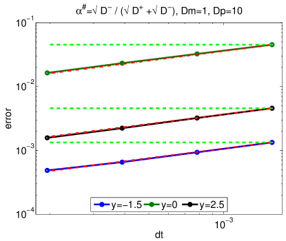
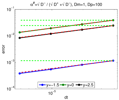
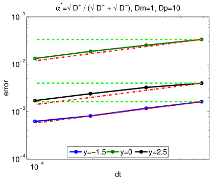
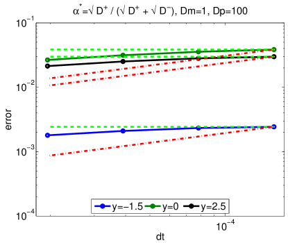
Figure 4: Error for the SDE-BE method demonstrating half order convergence.

7 Conclusions

In this paper we have introduced a natural one parameter family of possible interface conditions coupled to a diffusion problem, with discontinuous diffusion coefficient, in one spatial dimension. We then presented a reformation of the deterministic and the stochastic models which naturally allow the application of numerical discretization methods. In particular, we chose to use the immersed interface finite element method for the PDE. We extended standard energy estimates to show stability of the approach and derived error estimates for the backward Euler case. We demonstrated expected convergence via numerical examples. Finally, we introduced the corresponding SDE and developed an Euler-Maruyama scheme applicable to any one of the interface conditions. We proved existence, uniqueness and convergence of the numerical method under mild assumptions. Again, the rates of convergence were verified by numerical examples.

8 Appendix

In this section we provide some properties of the first passage time densities of one dimensional uniformly elliptic diffusion processes which imply the estimates for the density $r_{0}^{x}(s)$ of the first passage time before time $T$ at point $0$ of the process $Y^{(\alpha)}$. In addition, we will present an estimate for the number of visits of small balls by the Euler scheme.

The following Lemma is a combination of Theorem A.1 and Lemma A.5 in [27].

Lemma 8.1

Let $\gamma$ and $\mu$ be real valued functions such that $\gamma\in C^{k+2}_{b}(\mathbb{R})$ and $\mu\in C^{k+1}_{b}(\mathbb{R})$ for some non-negative integer $k$. Suppose that there is a positive constant $\lambda$ such that $\gamma(x)>\lambda$ for all $x$ and $Z(t)$ satisfies

$$Z(t)=Z_{0}+\int_{0}^{t}\mu(Z(s))ds+\int_{0}^{t}\gamma(Z(s))dB(s).$$

a, If $T>0$ and $x\neq 0$ then under $P^{x}$, the first passage time of $Z(t)$ at point $0$ before time $T$, $\tau_{0}(Z)\wedge T$, has a smooth density $r_{0}^{x}(s)$ which is of class $C^{k}((0,T])$.
b, In addition, if $k\geq 2$ then for all $0\leq\alpha<1$ there exists a constant $C$ such that

$$\int_{0}^{t}{1\over s^{\alpha}}r_{0}^{x}(t-s)ds\leq{C\over t^{\alpha}}\quad\text{for all $0\leq t\leq T$ and $x\neq 0$}.$$

We also have the following estimate from [27] (See Lemma A.6).

Lemma 8.2

There exists a positive constant $\tilde{C}$ such that for $0\leq\alpha\leq 1$ and any function $H$ bounded on $[0,T]$, continuously differentiable on $(0,T]$ satisfying

$$H(0)=0,\quad|H^{\prime}(s)|\leq{C_{H}\over s^{\alpha}}\,\,\forall s\in(0,T]$$

we have

$$\Big{|}{\partial\over\partial x}\int_{0}^{t}r_{0}^{x}(t-s)H(s)ds\Big{|}\leq C_{H}\tilde{C},\quad\Big{|}{\partial^{2}\over\partial x^{2}}\int_{0}^{t}r_{0}^{x}(t-s)H(s)ds\Big{|}\leq C_{H}\tilde{C}\Big{(}1+{1\over t^{\alpha}}\Big{)},$$

for all $t\in(0,T]$ and $x\neq 0$.

Next, let $W(\cdot)$ be a $m$-dimensional standard Brownian motion on a filtered probability space $(\Omega,\mathcal{F},\mathcal{F}_{t},P)$. Assume that $b(\cdot)$ and $\sigma(\cdot)$ are two progressive measurable processes taking values in $\mathbb{R}^{d}$ and in the space of real $d\times m$ matrices, and $X(\cdot)$ is the $\mathbb{R}^{d}$-valued process satisfying

$$X(t)=X(0)+\int_{0}^{t}b(s)ds+\int_{0}^{t}\sigma(s)dW(s).$$ (8.1)

Assume that
Assumption (A). There exists a positive number $K\geq 1$ such that

$$\forall\,t\geq 0,\quad\|b(t)\|\leq K\quad P-\text{a.s.}$$ (8.2)

and

$$\forall\,0\leq s\leq t,\quad{1\over K^{2}}\int_{s}^{t}\psi(s)ds\leq\int_{s}^{t}\psi(s)\|\sigma\sigma^{*}\|ds\leq K^{2}\int_{0}^{t}\psi(s)ds$$ (8.3)

for all positive locally integrable function $\psi$ on $\mathbb{R}^{+}$.

Assumption (B). $f$ is an increasing function in $C^{1}([0,T),\mathbb{R}^{+})$ such that $f^{\alpha}$ is integrable on $[0,T)$ for all $1\leq\alpha<2$. In addition, there exists $1<\nu<1+\eta$ where $\eta={1\over 4K^{4}}$ such that

$$\int_{0}^{T}f^{2\nu-1}(s)f^{\prime}(s){(T-s)^{1+\eta}\over s^{\eta}}ds<\infty.$$ (8.4)

Notice that (8.3) is satisfied if $\sigma$ is a bounded continuous process. The Assumption (B) is satisfied if $f(t)={1\over\sqrt{T-t}}$ and $\nu=1+{1\over 8K^{4}}$. We have the following estimate for the number of visits of small balls.

Theorem 8.3 (Theorem A.9 from [27])

Assume (A) and (B). Let $X(\cdot)$ be as in (8.1). Then there exists a constant $C>0$ depending only on $\nu,K$ and $T$ such that for all $\xi\in\mathbb{R}^{d}$ and $0<\epsilon<1/2$, there exists $h_{0}>0$ satisfying

$$\forall\,h\leq h_{0},\quad h\sum_{k=0}^{\lfloor T/h\rfloor-1}f(kh)P\big{(}\|X(kh)-\xi\|\leq h^{1/2-\epsilon}\big{)}\leq Ch^{1/2-\epsilon}.$$ (8.5)

References

- [1] M. A. Aizen, P. Feinsinger, G. A. Bradshaw, and P. Marquet. Bees not to be? Responses of insect pollinator faunas and flower pollination to habitat fragmentation. Ecological Studies, pages 111–130, 2003.
- [2] T. A. Appuhamillage, V. A. Bokil, E. Thomann, E. Waymire, and B. Wood. Skew dispersion and continuity of local time. Submitted, 2013.
- [3] T. A. Appuhamillage, V. A. Bokil, E. Thomann, E. Waymire, and B. D. Wood. Solute transport across an interface: A fickian theory for skewness in breakthrough curves. Water Resour. Res., 46(W07511, doi:10.1029/2009WR008258), 2010.
- [4] T. A. Appuhamillage, V. A. Bokil, E. Thomann, E. Waymire, and B. D. Wood. Occupation and Local Times for Skew Brownian Motion with Applications to Dispersion Across an Interface. Annals of Applied Probability, 21(1):183–214, 2011. DOI: 10.1214/10-AAP691.
- [5] T. A. Appuhamillage, V. A. Bokil, E. A. Thomann, E. C. Waymire, and B. D. Wood. First passage times and breakthrough curves associated with interfacial phenomena. Arxiv preprint arXiv:1106.4350, August 2011.
- [6] C. Attanayake and D. Senaratne. Convergence of an immersed finite element method for semilinear parabolic interface problems. Applied Mathematical Sciences, 5(3):135–147, 2011.
- [7] S Azaele, A. Maritan, E. Bertuzzo, I. Rodriguez-Iturbe, and A. Rinaldo. Stochastic dynamics of cholera epidemics. Physical Review E, 81(DOI: 10.1103/PhysRevE.81.051901):051901–1 to 05901–6, 2010.
- [8] R. S. Cantrell and C. Cosner. Diffusion models for population dynamics incorporating individual behavior at boundaries: Applications to refuge design. Theoretical Population Biology, 55(2):189–207, 1999.
- [9] R. S. Cantrell and C. Cosner. Spatial ecology via reaction-diffusion equations, volume 7. Wiley, 2003.
- [10] A. Einstein. Investigations on the Theory of the Brownian Movement. Dover Pubns, 1956.
- [11] P. Étoré. On random walk simulation of one-dimensional diffusion processes with discontinuous coefficients. Preprint, Institut Élie Cartan, Nancy, France. Electron. J. Probab. To appear, 2005.
- [12] P. Étoré and M. Martinez. Exact simulation of one-dimensional stochastic differential equations involving the local time at zero of the unknown process. Arxiv preprint arXiv:1102.2565, 2011.
- [13] R. Glowinski, T. W. Pan, and J. Périaux. A fictitious domain method for external incompressible viscous flow modeled by Navier-Stokes equations. Comp. Math. Appl Mech. Eng., 112:113–148, 1994.
- [14] J. M. Harrison and L. A. Shepp. On skew Brownian motion. The Annals of probability, pages 309–313, 1981.
- [15] K. Itô and H. P. McKean. Brownian motions on a half line. Illinois journal of mathematics, 7(2):181–231, 1963.
- [16] A. Lejay. Monte carlo methods for discontinuous media. Pau, France, 2009. 3rd International Conference on Approximation Methods and Numerical Modeling in Environment and Natural Resources (MAMERN09).
- [17] A. Lejay. Simulation of a stochastic process in a discontinuous, layered media. hal.archives-ouvertes.fr, 2011.
- [18] A. Lejay and M. Martinez. A scheme for simulating one-dimensional diffusion processes with discontinuous coefficients. Annals of Applied Probability, 16(1):107–139, 2006.
- [19] R. J. Leveque and Z. Li. The immersed interface method for elliptic equations with discontinuous coefficients and singular sources. SIAM Journal on Numerical Analysis, 31(4):1019–1044, 1994.
- [20] Z. Li. The immersed interface method using a finite element formulation. Applied Numerical Mathematics, 27(3):253–267, 1998.
- [21] Z. Li. An overview of the immersed interface method and its applications. Taiwanese J. Mathematics, 7(1):1–49, 2003.
- [22] Zhilin Li and Kazufumi Ito. The immersed interface method: numerical solutions of PDEs involving interfaces and irregular domains, volume 33. Siam, 2006.
- [23] T. Lin, Y. Lin, and W. Sun. Error estimation of a class of quadratic immersed finite element methods for elliptic interface problems. Discrete and Continuous Dynamical Systems Series B, 7(4):807, 2007.
- [24] F. Lutscher, M. A. Lewis, and E. McCauley. Effects of heterogeneity on spread and persistence in rivers. Bulletin of Mathematical Biology, DOI 10.1007/s11538-006-9100-1, 2006.
- [25] F. Lutscher, E. Pachepsky, and M. A. Lewis. The effect of dispersal patterns on stream populations. SIAM Review, 47(4):749–772, 2005.
- [26] M. Martinez and D. Talay. Discretization of one-dimensional stochastic differential equations whose generators are divergence form with a discontinuous coefficient. Comptes Rendus Mathematique, 342(1):51–56, 2006.
- [27] M. Martinez and D. Talay. One-dimensional parabolic diffraction equations: pointwise estimates and discretization of related stochastic differential equations with weighted local times. Electron. J. Probab., 17(27):1–32, 2012.
- [28] R. P. Matano and E. D. Palma. On the upwelling of downwelling currents. Journal of Physical Oceanography, 38(11):2482 – 2500, 2008.
- [29] D. Mayer, J. Reiczigel, and F. Rubel. A Lagrangian particle model to predict the airborne spread of foot-and-mouth disease virus. Atmospheric Environment, 42:466–479, 2008.
- [30] R. Mittal and G. Iaccarino. Immersed boundary methods. Annual review of fluid mechanics, 37:239–261, 2005.
- [31] C. S. Peskin. The immersed boundary method. Acta Numerica, 11:479–517, 2003.
- [32] J. Reiczigel, K. Brugger, F. Rubel, N. Solymosi, and Z. Lang. Bayesian analysis of a dynamical model for the spread of the usutu virus. Stochastic Environmental Research and Risk Assessment, 24:455–462, 2010.
- [33] L. Ries and D. M. Debinski. Butterfly responses to habitat edges in the highly fragmented prairies of central iowa. Journal of Animal Ecology, 70(5):840–852, 2001.
- [34] C. B. Schultz and E. E. Crone. Edge-mediated dispersal behavior in a prairie butterfly. Ecology, 82(7):1879–1892, 2001.
- [35] H. Seno and S. Koshiba. A mathematical model for invasion range of population dispersion through a patchy environment. Biological Invasions, 7(DOI 10.1007/s10530-005-5211-0):757–770, 2005.
- [36] J. G. Skellam. Random dispersal in theoretical populations. Biometrika, 38(1/2):196–218, 1951.
- [37] E. Süli. Lecture notes on finite element methods for partial differential equations. Mathematical Institute, University of Oxford, December 2012.
- [38] V. Thomée. Galerkin finite element methods for parabolic problems, volume 25. Springer, 2006.
- [39] P. Turchin and P. Kareiva. Aggregation in aphis varians: an effective strategy for reducing predation risk. Ecology, pages 1008–1016, 1989.
- [40] J. B. Walsh. A diffusion with a discontinuous local time. Asterisque, 52–53:37–45, 1978.
- [41] A. Wiegmann and K. P. Bube. The immersed interface method for nonlinear differential equations with discontinuous coefficients and singular sources. SIAM Journal on Numerical Analysis, 35(1):177–200, 1998.
- [42] Z. Yu, X. Shao, and A. Wachs. A fictitious domain method for particulate flows with heat transfer. Journal of Computational Physics, 217(2):424–452, 2006.
- [43] S. Zhao and G. W. Wei. High-order FDTD methods via derivative matching for Maxwell’s equations with material interfaces. Journal of Computational Physics, 200(1):60–103, 2004.
- [44] Y. C. Zhou, S. Zhao, M. Feig, and G. W. Wei. High order matched interface and boundary method for elliptic equations with discontinuous coefficients and singular sources. Journal of Computational Physics, 213(1):1–30, 2006.