Tree Nash Equilibria in the
Network Creation Game

Abstract

In the network creation game with $n$ vertices, every vertex (a player) buys a set of adjacent edges, each at a fixed amount $\alpha>0$. It has been conjectured that for $\alpha\geq n$, every Nash equilibrium is a tree, and has been confirmed for every $\alpha\geq 273\cdot n$. We improve upon this bound and show that this is true for every $\alpha\geq 65\cdot n$. To show this, we provide new and improved results on the local structure of Nash equilibria. Technically, we show that if there is a cycle in a Nash equilibrium, then $\alpha<65\cdot n$. Proving this, we only consider relatively simple strategy changes of the players involved in the cycle. We further show that this simple approach cannot be used to show the desired upper bound $\alpha<n$ (for which a cycle may exist), but conjecture that a slightly worse bound $\alpha<1.3\cdot n$ can be achieved with this approach. Towards this conjecture, we show that if a Nash equilibrium has a cycle of length at most 10, then indeed $\alpha<1.3\cdot n$. We further provide experimental evidence suggesting that when the girth of a Nash equilibrium is increasing, the upper bound on $\alpha$ obtained by the simple strategy changes is not increasing. To the end, we investigate the approach for a coalitional variant of Nash equilibrium, where coalitions of two players cannot collectively improve, and show that if $\alpha\geq 41\cdot n$, then every such Nash equilibrium is a tree.

1 Introduction

Network creation game has been introduced by Fabrikant et al. [8] as a formal model to study the effects of strategic decisions of economically motivated agents in decentralized networks such as the Internet. In such networks, local decisions including those about infrastructure are decided by autonomous systems. Autonomous systems follow their own interest, and as a result, their decisions may be sub-optimal for the whole society. Network creation games allow to formally study the structure of networks created in such a manner, and to compare them with potentially optimal networks (optimal with respect to the whole society).

In the network creation game, there are $n$ players $V=\{1,\ldots,n\}$, each representing a vertex of an undirected graph. The strategy $s_{i}$ of a player $i$ is to create (or buy) a set of adjacent edges, each at a fixed amount $\alpha>0$. The played strategies $s=(s_{1},\ldots,s_{n})$ collectively define an edge-set $E_{s}$, and thus a graph $G_{s}=(V,E_{s})$. The goal of every player is to minimize its cost $c_{i}$, which is the amount paid for the edges (creation cost), plus the total distances of the player to every other node of the resulting network $G$ (usage cost), i.e.,

$$c_{i}(s)=\alpha\cdot|s_{i}|+\sum_{j=1}^{n}\text{dist}(i,j)\text{,}$$

where $\text{dist}(i,j)$ denotes the distance between $i$ and $j$ in the resulting network $G$.

A strategy vector $s=(s_{1},\ldots,s_{n})$ is a Nash equilibrium if no player $i$ can change the set $s_{i}$ of created edges to another set $s_{i}^{\prime}$ and improve its cost $c_{i}$. Abusing the definition, the resulting graph $G_{s}$ itself is called a Nash equilibrium, too, and we define its (social) cost $c(G)$ to be the cost $c(s)$, i.e., the cost of the corresponding strategy vector $s$. The social cost $c(s)$ of strategy vector $s$ is the sum of the individual costs, i.e., $c(s)=\sum_{i=1}^{n}c_{i}(s)$. It is a trivial observation to see that in any Nash equilibrium $G_{s}$, no edge is bought more than once. From now on, we only consider such strategy vectors, and observe then that

$$c(s):=\sum_{i=1}^{n}c_{i}(s)=\alpha\cdot|E_{s}|+\sum_{i=1}^{n}\sum_{j=1}^{n}d(i,j)\text{.}$$

A graph $G=(V,E)$ can be created by many strategy vectors $s$ (precisely in $2^{|E|}$ many ways, because every edge in $E$ can be bought by exactly one of its endpoints), but each of such realizations has the same social cost. Graph $G^{*}=(V,E)$ is an optimum graph, if it minimizes the social cost $c(s)$ (for any strategy vector $s$ for which $G_{s}=G$).

Let $\mathcal{N}$ denote the set of all Nash equilibria of a network creation game on $n$ vertices and edge-price $\alpha$. The price of anarchy (PoA) of the network creation game is the ratio

$$\text{PoA}=\max_{s\in\mathcal{N}}\frac{c(G_{s})}{c(G^{*})}\text{.}$$

Price of anarchy expresses the (worst-case) loss of the quality of a network that the society could achieve.

In a series of papers [8, 1, 6, 9] it has been shown that the price of anarchy of the network creation game is $O(1)$, i.e., a constant independent of both $n$ and $\alpha$, for every value $\alpha>0$ with the exception of the range $n^{1-\varepsilon}<\alpha<273\cdot n$, where $\varepsilon=\Omega(\frac{1}{\log n})$. For the value of $\alpha$ with $n^{1-\varepsilon}<\alpha<273\cdot n$, an upper bound of $2^{\sqrt[n]{\log n}}$ on the price of anarchy is known (while no Nash equilibrium with considerably large social cost is known). It is conjectured, however, that the price of anarchy is constant also in this range of $\alpha$. It remains a major open problem to confirm or disprove this conjecture. It is certainly of interest to note that there are several variants of the network creation game (see, e.g., [2, 4, 7, 3]), but in none of these, with the exception of [5], the price of anarchy could be shown to be constant.

Understanding the structure of Nash equilibria has proven to be important in bounding the price of anarchy. Fabrikant et al. [8] showed that the social cost of any tree $G$ in Nash equilibrium is upper-bounded by $O(1)\cdot c(G^{*})$. Therefore, the price of anarchy is $O(1)$ for all values of $\alpha$ for which every Nash equilibrium is a tree. It has been shown that every Nash equilibrium is a tree for all values of $\alpha$ greater than $n^{2}$, $12n\log n$, and $273n$, respectively, in [8],[1], and [9]. It has been conjectured that every Nash equilibrium is a tree for every $\alpha\geq n$. Since for $\alpha=n/2$, non-tree Nash equilibria are known, this tree conjecture is asymptotically tight.

In this paper, we make steps in the direction of resolving the tree conjecture. We first tighten the tree conjecture and provide a construction of a non-tree Nash equilibrium for every $\alpha=n-3$ (thus, showing that, asymptotically, one cannot hope to show that every Nash equilibrium is a tree for some value $\alpha<n$). We then apply a “linear-programming-like” approach to show that for $\alpha\geq 65n$, every Nash equilibrium is a tree. To show this, we obtain new structural results on Nash equilibria and combine them with the previous approach of [9]. Towards the end, we make further steps towards the conjecture. We show that if $\alpha\geq n$, then there is no non-tree Nash equilibrium containing exactly one cycle. We then apply the “linear-programming-like” approach again to show that the girth of every non-tree Nash equilibrium (for any $\alpha\geq n$) is at least 6. Using the same ideas, we show that if a non-tree Nash equilibrium has girth at most 10, then $\alpha\leq 1.3n$. By further experimental results, we conjecture that this holds for any girth, i.e., that non-tree Nash equilibria can appear only for $\alpha\leq 1.3n$.

2 Preliminaries

In the following, we will often denote the considered Nash equilibrium graph $G_{s}=(V,E_{s})$ of a network creation game with $\alpha>0$ simply as $G=(V,E)$. Even though the graph $G_{s}$ is undirected, we will often direct the edges to express the identity of the player which bought the edge in $s$; An edge $\{u,v\}$ directed from $u$ to $v$ denotes the fact that $u$ bought/created the edge in $s$.

Every non-tree $G$ contains a cycle. Let $c$ be the length of a shortest cycle $C$ in $G$, and let $a_{0},a_{1},\ldots,a_{c-1}$ be the players that form one such shortest cycle, and where $\{a_{i},a_{i+1}\}\in E$ for every $i=0,1,\ldots,c-1$ (where indices on vertices of the cycle are in the whole paper to be understood modulo $c$). Observe the crucial property of a shortest cycle $C$: the distance between $a_{i}$ and $a_{j}$ in the graph $G$ is equal to the distance between $a_{i}$ and $a_{j}$ on the cycle $C$.

We will consider the players on the cycle $C$ and their strategy-changes that involve only the $c$ edges of the cycle. For each strategy-change $s_{a_{i}}^{\prime}$ of player $a_{i}$, we obtain an inequality $c_{i}(s)\leq c_{i}(s_{1},\ldots,s_{a_{i}}^{\prime},\ldots,s_{n})$ stating simply the fact that in a Nash equilibrium $s$, player $a_{i}$ cannot improve by changing its strategy. We will often express such an inequality in the form of “SAVINGS” $\leq$ “INCREASE”, where “SAVINGS” denotes the parts of $c_{i}(s)$ that decreased their value in $c_{i}(s^{\prime})$, and “INCREASE” denotes the parts of $c_{i}(s)$ that increased their value in $c_{i}(s^{\prime})$. For example, assume that $a_{i}$ buys the edge $e=\{a_{i},a_{i+1}\}$ (i.e., $e\in s_{i}$), and let us consider the strategy change where $a_{i}$ deletes the edge $e$ (i.e., $s_{i}^{\prime}=s_{i}\setminus\{e\}$). Recall that $c_{i}(s)=\alpha\cdot|s_{i}|+\sum_{j}d(i,j)$. Then, in such a strategy change, the “SAVINGS” are clearly on the edge-creation side, i.e., the player $a_{i}$ saves $\alpha$ for not paying for the edge $e$. At the same time, some distances of player $i$ may have increased – the distance to a vertex $v$ increases, if in $G_{s}$ every shortest path from $a_{i}$ to $v$ uses the deleted edge $e$. But the distance to $v$ could have increased by at most $c-2$ (as before, $a_{i}$ needed to go to vertex $a_{i+1}$ but now the vertex $a_{i+1}$ can be reached “around” the cycle). Because of the Nash equilibrium property of $s$, we have “SAVINGS” $\leq$ “INCREASE”, which implies $\alpha\leq(c-2)(n-1)$ (as the distance to at most $n-1$ vertices could have increased).

In the following, we will use slightly more involved forms of the just described inequalities. For that reason, we will partition the vertices according to their distances to the vertices from the cycle. Let us fix a vertex $v\in V$. Let $G\setminus C$ be the graph $G$ without the $c$ edges of the cycle $C$. Let us denote the distances of $v$ to the vertices $a_{0},a_{1},\ldots,a_{c-1}$ in $G\setminus C$ by the vector $d(v)=(d_{0},d_{1},\ldots,d_{c-1})$, respectively, where $d_{i}=\infty$ if $a_{i}$ and $v$ are disconnected in $G\setminus C$. We call $d_{i}$ the outer distance of $v$ to $a_{i}$ in the Nash equilibrium $G$, and $d$ the vector of outer distances of $v$ in $G$. We now partition the vertices of $V$ by this vector of outer distances. We will coarsen the partition in the following way. Observe that $d_{s}(a_{i},v)$ in $G_{s}$ is now equal to $\min_{j}(d_{s}(a_{i},a_{j})+d_{j})$, because there always is a shortest path from $a_{i}$ to $v$ that first uses a part of the cycle $C$ (until vertex $a_{j}$), leaves $C$ and never comes back to $C$. Therefore, $\min_{j}d_{j}\leq d_{s}(a_{i},v)\leq(c-1)+\min_{j}d_{j})$. Moreover, for any strategy change $s_{i}^{\prime}$ of player $a_{i}$ which leaves $a_{i}$ connected by an edge to a vertex of $C$, we still have $\min_{j}d_{j}\leq d_{s^{\prime}}(a_{i},v)\leq(c-1)+\min_{j}d_{j}$ (because there is a path from $a_{i}$ to the vertex $a_{j}$ of smallest entry $d_{j}$ using the edge and the remaining of the cycle). Because we are interested in the changes of the distances from $a_{i}$, i.e., in the value of $\Delta:=d_{s^{\prime}}(a_{i},v)-d_{s}(a_{i},v)$, we can normalize the vector $d(v)$ by subtracting $\min_{j}d_{j}$ from each of the elements $d_{0},d_{1},\ldots,d_{c-1}$ (which does not change the value of $\Delta$). Observe that after the normalization, there is an entry $d_{i}$ equal to zero. We will “normalize” the entries further more. Since we are interested in the value $\Delta$, we can handle all entries $d_{j}\geq c-1$ in the same way: they do not have any influence on $\Delta$ at all (no shortest path from vertex $a_{i}$, $i\neq j$, will ever use $a_{j}$ to reach vertex $v$). We will therefore further modify the vector $d$ by substituting every entry $d_{j}\geq c-1$ with the value $c-1$.

Figure 1: Non-tree Nash equilibrium for $n=2s+3$ players and $\alpha=n-3$. An edge directed from a node $u$ to a node $v$ denotes that $u$ buys the edge.

This gives partition of all vertices into groups $V_{d}$, where each group has associated vector of “normalized” outer distances $d=(d_{0},\cdots,d_{c-1})$, one of the distances is necessarily equal to $0$ and all the distances are upper bounded by $c-1$. Vertices which have vector of outer distances $d^{\prime}$ containing numbers greater than $c-1$ are associated with the group having a vector $d^{\prime\prime}$ obtained from $d^{\prime}$ where all entries greater than $c-1$ are changed to $c-1$. In this way, there are $t=c^{c}-(c-1)^{c}$ groups. We denote the set of all “normalized” distance vectors by $D$. Trivially, as $V_{d}$, $d\in D$, form a partition of $V$, $\sum_{d\in D}|V_{d}|=n$.

3 Bounds on $\alpha$ for existence of cycles

We first give in Fig. 1 a construction of a non-tree Nash equilibrium graph for $n=2s+3$ vertices, and $\alpha=2s=n-3$, for any integer $s$. This thus shows that the conjecture “for $\alpha\geq n$, all Nash equilibria are trees” cannot be improved to “for $\alpha\geq(1-\varepsilon)n$, all Nash equilibria are trees”. We now proceed and give a lower bound on the length of a shortest cycle in any Nash equilibrium.

Theorem 1

The length $c$ of a shortest cycle $C$ in any Nash equilibrium is at least $\frac{2\alpha}{n}+2$.

Proof. We distinguish two cases. First, assume that there is a player, which buys both its adjacent edges on the cycle $C$. Without loss of generality assume that this player is $a_{0}$. Consider the strategy change where $a_{0}$ deletes both these edges $\{a_{0},a_{1}\}$ and $\{a_{0},a_{c-1}\}$ and buys an edge towards player $a_{i}$ on the cycle, $i=2,\ldots,c-2$. The player cannot improve by such a change, and therefore “SAVINGS” $\leq$ “INCREASE”. Here, the player saves at least $\alpha$ (by buying one edge less). Let us denote the increase of distances of player $a_{0}$ to the players of the group $V_{d}$ by $c_{i,d}$. Then we get that $\alpha\leq\sum_{d\in D}\delta_{i,d}|V_{d}|$. Summing up all the $c-3$ inequalities, one for every $i$, we get $(c-3)\alpha\leq\sum_{i=2}^{c-2}\sum_{d}\delta_{i,d}|V_{d}|$.

We now show that for every $d$, the coefficient $\sum_{i}\delta_{i,d}$ at $|V_{d}|$ is at most $(c-2)(c-3)/2$. Consider arbitrary $d=(d_{0},d_{1},\ldots,d_{c-1})$ of the outer distances of the vertices in $V_{d}$. Clearly, the strategy change of $a_{0}$ increases its distances to $V_{d}$ iff every shortest path from $a_{0}$ to $V_{d}$ goes through the deleted edges. Thus, we can assume (for the worst-case) that $d_{0}=c-1$. Assume that one shortest path (in $G_{s}$) leaves the cycle at $a_{e}$, $e\in\{1,\ldots,c-2\}$. In the new graph $G_{s^{\prime}}$, player $a_{0}$ can always use the new edge $\{a_{0},a_{i}\}$ and then go to $a_{e}$ on the remainder of the cycle $C$. Thus, the increase of distances $\delta_{i,d}$ is at most $(1+|i-e|)-1=|i-e|$. In total, we obtain $\sum_{i=2}^{c-2}\delta_{i,d}\leq\sum_{i}|i-e|\leq\sum_{i}(i-1)=(c-3)(c-2)/2$, as claimed. Now, since $\sum_{d\in D}|V_{d}|=n$, we finally get that $\alpha\leq\frac{(c-2)}{2}n$, which gives the claimed $c\geq\frac{2\alpha}{n}+2$.

Consider now the second case where no player buys two of its adjacent edges in $C$, i.e., every player buys exactly one edge. Without loss of generality assume that every player $a_{i}$ buys the edge $\{a_{i},a_{i+1}\}$. For each player $i$, we consider the strategy change of deleting the edge $\{a_{i},a_{i+1}\}$. Similarly to the previous case, we obtain $\alpha\leq\sum_{d\in D}\delta_{i,d}|V_{d}|$. Summing for every $i$, we get $c\alpha\leq\sum_{i=0}^{c-1}\sum_{d}\delta_{i,d}|V_{d}|$. We show this time that $\sum_{i=0}^{c-1}\delta_{i,d}$, the coefficient at $|V_{d}|$, is upper bounded by $1+2+\dots+(c-2)=(c-2)(c-1)/2$. Consider an arbitrary $d=(d_{0},\ldots,d_{c-1})\in D$, and assume without loss of generality that $d_{0}=0$. For every player $a_{i}$, $\delta_{i,d}$ is at most $i-1$, because the worst-case increase in a distance of player $a_{i}$ to vertices $V_{d}$ happens when all shortest paths from $a_{i}$ used the deleted edge $\{a_{i},a_{i+1}\}$. But because after the deletion, there is an alternative path from $a_{i}$ to $V_{d}$ using $a_{0}$, the increase is at most $i-1$. Thus, summing over all $i$, the total increase in distances to $V_{d}$ is at most $0+1+2+\dots+(c-2)=(c-2)(c-1)/2$ as claimed. Plugging this into our inequality, $c\alpha\leq\sum_{i}\sum_{d}\delta_{i,d}|V_{d}|$ and using the fact that $\sum_{d}|V_{d}|=n$, we obtain that $c>\frac{2\alpha}{n}+2$.

$\Box$

Let $H$ be a non-trivial biconnected component of a non-tree Nash equilibrium, i.e., an induced subgraph of $H$ of at least three vertices containing no bridge. For any vertex $v\in H$, let $S(v)$ be the set of vertices which do not belong to $H$, and which have $v$ as the closest vertex among all vertices in $H$. For any vertex $u\in H$, we define $deg_{H}(u)$ to be the degree of vertex $u$ in the graph induced by $H$. Furthermore, we define $N_{k}(u)$ to be the $k$-th neighborhood of $u$ in $H$, i.e., $N_{k}(u):=\{w\in H\ |\ d(u,w)\leq k\}$. The following lemma has been shown in [9]. We will use it to prove the subsequent lemma.

Lemma 1 ([9])

If $u,v\in V(H)$ are two vertices in $H$ with $d(u,v)\geq 3$ such that $u$ buys the edge to its adjacent vertex $x$ in a shortest $u-v$-path and $v$ buys the edge to its adjacent vertex $y$ in that path, then $deg_{H}(x)\geq 3$ or $deg_{H}(y)\geq 3$.

Lemma 2

If $H$ is a biconnected component of $G$, then for any vertex $u$, its neighborhood $N_{5}(u)$ in $H$ contains a vertex $v$ with $deg_{H}(v)\geq 3$.

Proof. Assume that this is not true. Then the 5-neighborhood $N_{5}(u)$ of vertex $u$ is formed by two disjoint paths. (The case that the 5-neighborhood forms a cycle is excluded by Proposition 1 stating that no Nash equilibrium for $\alpha>n$ contains exactly one cycle). We consider two cases. First, we will assume that at least one of the two paths starting at $u$ is directed away from $u$ (see Fig. 2(a)). In the second case, in each of the two paths, there has to be a vertex which buys an edge towards $u$. It follows from Lemma 1 that these two vertices are the two neighbors of $u$ in $N_{5}(u)$ (see Fig. 2(b)).

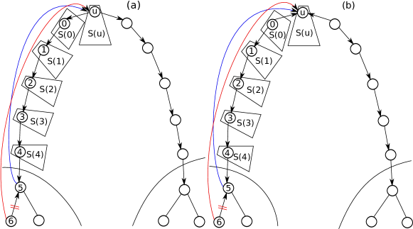
Figure 2: The 5-Neighborhood $N_{5}(u)$ of vertex $u$.

In the first case, there is a sequence of five edges directed away from $u$, with the naming like in Fig. 2(a)). Let $s_{u}:=|S(u)|$, $s_{i}=|S(i)|$ for $0\leq i\leq 4$.

Then,

$$s_{0}\geq s_{1}+s_{2}+s_{3}+s_{4},s_{1}\geq s_{2}+s_{3}+s_{4},s_{2}\geq s_{3}+s_{4},s_{3}\geq s_{4},s_{4}\geq k\text{,}$$ (1)

where $k$ is the number of vertices which are descendants of vertex $5$ in the breadth-first-search (BFS) tree rooted at vertex $3$. We can obtain these inequalities by considering the following strategy changes of the players $u$ and $i$, $0\leq i\leq 3$: delete the edge directed away from $u$, and buy a new edge to the next vertex in the sequence; now simply apply the “SAVINGS” $\leq$ “INCREASE” principle.

We first assume that vertex $5$, the neighbor of vertex $4$ in $H$, has degree at least 3 in $H$ (i.e., it has at least two children in the BFS tree rooted at vertex 3). The case when the degree-3 vertex appears later along the path is easier and will be discussed later. We now distinguish two cases. First, we assume that one of the children of vertex $5$ in the considered BFS tree buys an edge to vertex $5$. Let us call it vertex $6$. The other case is when vertex $5$ buys all the edges to its children.

Consider the following strategy change: vertex $6$ deletes an edge towards vertex 5 and buys new edge towards vertex $u$. This decreases its distance cost at least to vertices in $S(0)$ by 4, and to vertices in $S(1)$ by 2, whilst increases distances to vertices in the set of descendants of $5$ in the BFS tree rooted at $3$ by at most $6$, to the vertices in $S(4)$ by $4$ and to the vertices in $S(3)$ by two. By this strategy change distance from vertex 6 to any other vertex is not increased, because vertex $u$ is located deeper than vertex $6$ in the BFS tree rooted at vertex $3$. But then according to the chain of inequalities (1) we get $4s_{0}+2s_{1}>6k+4s_{4}+2s_{3}$, and thus the player $6$ can improve, a contradiction.

In the case where vertex 5 buys all edges towards its children, consider the following strategy change of vertex 5: delete all the edges to its children (in the considered BFS tree) and buy one edge to vertex $u$. By this, the “SAVINGS” are at least $\alpha$. Furthermore, since $H$ is biconnected, the graph remains connected. Distances from vertex $5$ are increased only to vertices in the set $K$ – the set of the vertices which are descendants of vertex 5 in the BFS tree rooted at vertex 3. This “INCREASE” is at most $2\cdot diam(H)$, where $diam(H)$ is the diameter of $H$. By the “SAVINGS” $\leq$ “INCREASE” principle, we get that $\alpha\leq 2\cdot diam(h)k$. At the same time, $\alpha\geq(rad(H)-1)s_{0}$, where $rad(H)$ is the radius of $H$, as otherwise a vertex at distance $rad(H)$ from vertex $0$ could buy an edge towards vertex $0$ and decrease its cost. Combining these two inequalities with the inequality $s_{0}\geq 8k$, which is obtained from (1), we get that $8(rad(H)-1)k\leq 2\cdot diam(H)k\leq 4\cdot rad(H)k$, which is a contradiction.

The second case depicted in Fig. 2(b) is analyzed in the very same way, the only change is that now the heaviest component is $S(u)$. The chain of inequalities is similar to (1):

$$s_{u}\geq s_{0}+s_{1}+s_{2}+s_{3},s_{1}\geq s_{2}+s_{3}+s_{4},s_{2}\geq s_{3}+s_{4},s_{3}\geq s_{4},s_{4}\geq k\text{,}$$ (2)

where the notation is the same as in the first case. We obtain that $s_{u}\geq 7k$, and subsequently, arguing about the vertex at distance $rad(H)$ from $u$, the contradiction $7(rad(H)-1)k\leq 2\cdot diam(H)k\leq 4rad(H)k$.

Finally, if there is a longer sequence of vertices with degree $2$ than the considered sequence of length 5 of edges directed away from $u$, then we can only consider the last 5 edges (all directed away from $u$) and apply the very same reasoning.

$\Box$

We can strengthen the result if we consider stronger version of a Nash equilibrium in which no coalition of two players can change their strategies and improve their overall cost.

We call such an equilibrium a $2$-coalitional Nash equilibrium.

Lemma 3

The 3-neighborhood $N_{3}(u)$ of any vertex $u$ of a biconnected component $H$ of a 2-coalitional Nash equilibrium has a vertex of degree at least 3.

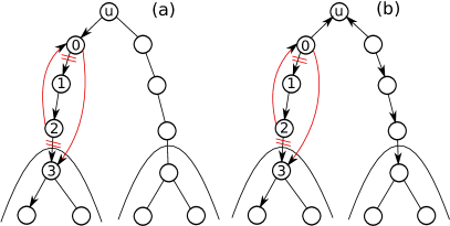
Figure 3: The 3-Neighborhood $N_{3}(u)$ of vertex $u$.

Proof. Assume the converse. Similarly to the proof of Lemma 2, there are two different cases of how the neighborhood of vertex $u$ looks like (see Fig. 3(a) and (b); notation is also the same as in Lemma 2). In both cases consider the coalition of players $0$ and $2$. Consider the following strategy changes: player $0$ deletes edge $(0,1)$ and instead buys edge $(0,3)$, whilst player $2$ deletes edge $(2,3)$ and buys edge $(2,0)$. This strategy change does not change the player coalition’s creation cost (in terms of $\alpha$). Among the vertices $S(0),S(1),S(2)$ and $S(u)$ this strategy change decreases coalition’s usage cost by $s_{u}+s_{0}+s_{2}$ and increases by $s_{1}$. Other vertices are partitioned by their shortest distances to vertices $0$ and $2$, lets assume that for any vertex $v$ which does not belong to $S(0),S(1),S(2)$ or $S(u)$ shortest distance to vertex $0$ is $x$ and shortest distance to vertex $2$ is $y$. Obviously $|x-y|\leq 2$. If $|x-y|>0$ then there is no increase in the usage cost of coalition towards vertex $v$ by this strategy change. The only possibility of increase is when $x=y$, but in that case $v$ is the descendant of vertex $3$ in the BFS tree rooted at vertex $1$. Similarly to Lemma 2, we denote $k$ to be the number of vertices which are descendants of vertex $3$ in the BFS tree rooted at vertex $1$. Analogously to the proof of Lemma 2, the following inequalities hold for the case depicted in Fig. 3(a): $s_{0}\geq s_{1}+s_{2},s_{1}\geq s_{2}\mbox{ and }s_{2}\geq k\text{,}$ whilst for the case depicted in Fig. 3(b), we have $s_{u}\geq s_{0}+s_{1}+s_{2},s_{1}\geq s_{2},s_{2}\geq k$. In both cases $s_{u}+s_{0}+s_{2}>s_{1}+k$, which results in a contradiction.

$\Box$

The following two lemmas are crucial for proving the main result of the paper. The first lemma has been proven in [9]. The second lemma strengthens a similar lemma from [9]. Its proof uses the result of Theorem 1.

Lemma 4 ([9])

If the $t$-neighborhood of every vertex of a biconnected component $H$ of a Nash equilibrium contains a vertex of degree at least $3$, then the average degree of $H$ is at least $2+\frac{1}{3t+1}$.

Lemma 5

If $\alpha>n$, then the average degree of a biconnected component $H$ of a Nash equilibrium graph is at most $2+\frac{4n}{\alpha-n}$.

Proof. Among all vertices of the equilibrium graph $G$, consider a vertex with the smallest usage cost and let this vertex be $v$. Consider a BFS tree $T$ rooted in $v$. Let $T^{\prime}=T\cap H$. Then the average degree of $H$ is $deg(H)=\frac{2|E(T^{\prime})|+2|E(H)\setminus E(T^{\prime})|}{|V(T^{\prime})|}\leq 2+\frac{2|E(H)\setminus E(T^{\prime})|}{|V(T^{\prime})|}$. We now bound $|E(H)\setminus E(T^{\prime})|$. We consider vertices that buy an edge in $E(H)\setminus E(T^{\prime})$ and call them shopping vertices. It is easy to see that no shopping vertex buys more than 1 edge, because if any of them buys two or more edges, it is better for it to delete all of the edges and buy 1 new edge towards $v$: this decreases its creation cost by at least $\alpha$, whilst increases its usage cost by at most $n$. It is thus enough to bound the number of shopping vertices. For this, we prove that the distance in the tree $T^{\prime}$ between any two shopping vertices is lower bounded by $\frac{\alpha-n}{n}$, which then implies that there can not be too many shopping vertices. Namely, the number of shopping vertices is at most $\frac{2nV(T^{\prime})}{\alpha-n}$. Assigning every node from $H$ to the closest shopping vertex according to the distance in $T^{\prime}$ forms a partition of $H$, where every part contains exactly one shopping vertex. As the distance in $T^{\prime}$ between shopping vertices is at least $\frac{\alpha-n}{n}$, the size of every part is at least $\frac{\alpha-n}{2n}$.

We assume for contradiction that there is a pair of shopping vertices $u_{1}$ and $u_{2}$ such that $d_{T^{\prime}}(u_{1},u_{2})<\frac{\alpha-n}{n}$. Let $u_{1}=x_{1},\cdots,x_{k}=u_{2}$ be the unique path from $u_{1}$ to $u_{2}$ in $T^{\prime}$, and $(u_{1},v_{1})$ and $(u_{2},v_{2})$ be the edges bought by $u_{1}$ and $u_{2}$ in $E(H)\setminus E(T^{\prime})$. Observe first that vertices $v_{1}$ and $v_{2}$ are not descendants of any vertex $x_{i}$, otherwise paths $v_{j}-x_{i}$ and $x_{i}-u_{j}$ together with an edge $(u_{j},v_{j})$ form a cycle of length at most $2(d_{T^{\prime}}(u_{1},u_{2})+1)<\frac{2\alpha}{n}+2$ which contradicts Theorem 1. Thus, $x_{0}:=v_{1},x_{1},\ldots,x_{k},x_{k+1}:=v_{2}$ is a path. Since $x_{1}$ buys edge $(x_{0},x_{1})$ and $x_{k}$ buys edge $(x_{k},x_{k+1})$, there is a vertex $x_{i}$ such that $x_{i}$ buys both of its adjacent edges $(x_{i-1},x_{i})$ and $(x_{i},x_{i+1})$. Consider the following strategy change for player $x_{i}$: delete the two adjacent edges and buy a new edge to vertex $v$. In this way $x_{i}$ decreases its creation cost by $\alpha$.

We now show that $U_{\text{new}}(x_{i})$, the usage cost of $x_{i}$ in the new graph, is less than $U_{G}(x_{i})$, the usage cost in the original graph, plus $\alpha$, which gives a contradiction. It is easy to observe that $U_{\text{new}}(x_{i})\leq n+U_{\text{new}}(v)$, since $x_{i}$ can always go through $v$ in the new strategy to any vertex. We now consider $U_{\text{new}}(v)$. Note that only the vertices in the path $u_{1}-u_{2}$ and their descendants can increase their distance to $v$ by the strategy change of $x_{i}$. Let $y$ be any such vertex. If the closest ancestor of $y$ on the path is $x_{i}$, then $d_{\text{new}}(v,y)\leq d_{G}(v,y)$, so there is no increase. We assume, without loss of generality, that the closest ancestor (of $y$) $x_{j}$ has an index less than $i$, i.e., $j<i$. Then the following chain of inequalities and equalities hold: $d_{\text{new}}(v,y)\leq d_{\text{new}}(v,x_{0})+d_{\text{new}}(x_{0},x_{j})+d_{\text{new}}(x_{j},y)=d_{G}(v,x_{0})+d_{G}(x_{0},x_{j})+d_{G}(x_{j},y)$ (the inequality is a triangle inequality, whilst the equality holds because $x_{0}$ is not a descendant of any vertex on the path in the new graph). Since $d_{G}(v,y)=d_{G}(v,x_{j})+d_{G}(x_{j},y)$, the difference between new and initial distances is $d_{new}(v,y)-d_{G}(v,y)=d_{G}(v,x_{0})+d_{G}(x_{0},x_{j})-d_{G}(v,x_{j})\leq 2d_{G}(x_{0},x_{j})\leq d_{G}(u_{1},u_{2})\leq 2\cdot d_{T^{\prime}}(u_{1},u_{2})\leq\frac{2(\alpha-n)}{n}$ (where the latter inequality is implied by our assumption). We need to bound the number of possible $y$’s. Path $u_{1}-u_{2}$ does not go through vertex $v$, so the number of possible $y$’s is bounded by the size of the subtree of $T$ of a child of $v$ that contains this path. We prove that the size of any subtree of a child of $v$ in $T^{\prime}$ is at most $\frac{n}{2}$.

Consider any child $t$ of $v$ in $T$, and consider the subtree of $T$ rooted in $t$. Let the $b$ be the number of vertices in the subtree, and let $a$ be the number of other vertices of $T$. Let $c_{1}$ be the usage cost of $t$ in the subtree, and let $c_{2}$ be the usage cost of $v$ (!!) in the other part of the tree $T$. Then the usage cost of $t$ in $G$ is upper bounded by $c_{1}+a+c_{2}$, whilst the usage cost of $v$ is exactly $b+c_{1}+c_{2}$. Since $v$ is the vertex with the minimal usage cost, we have $c_{1}+a+c_{2}\geq b+c_{1}+c_{2}$. Since $a+b=n$, we get that $b\leq\frac{n}{2}$.

Since $y$ was chosen arbitrarily, the increase of the usage cost for $v$ is less than $\frac{n}{2}\frac{2(\alpha-n)}{n}=\alpha-n$, and therefore $U_{\text{new}}(v)<U_{G}(v)+\alpha-n$ which is a contradiction.

$\Box$

Combining Lemmas $2$ and $3$ with Lemmas $4$ and $5$ gives the main result.

Theorem 2

For $\alpha\geq 65n$ every Nash equilibrium graph is a tree.

Theorem 3

For $\alpha\geq 41n$ every 2-coalitional Nash equilibrium graph is a tree.

4 Small cycles and experimental results

In this section we consider equilibrium graphs that have small girth $c$, and show that they exist only for small values of $\alpha$. We start with an observation that limits the girth of equilibrium graphs containing exactly one cycle.

Proposition 1

Let $G$ be a Nash equilibrium graph containing a $k$-cycle $C=\{v_{0},v_{1},\ldots,v_{k-1}\}$, and $F$ the graph where the edges of $C$ are removed from $G$. If $F$ consists of $k$ connected components, then $k<6$.

Proof. Assume for contradiction that $k\geq 6$. For $0\leq i<k$ let $s_{i}>0$ denote the number of vertices in the connected component of $F$ which contains $v_{i}$. If the edge $(v_{0},v_{k-1})$ is bought by the player $v_{0}$, then she could replace $(v_{0},v_{k-1})$ by $(v_{0},v_{k-2})$. By doing this, her creation cost will remain the same, her distances to $s_{k-3}+s_{k-2}$ vertices decrease by 1, but her distances to $s_{k-1}$ vertices increase by 1. If the edge $(v_{0},v_{k-1})$ is bought by the player $v_{k-1}$, this player could replace $(v_{k-1},v_{0})$ by $(v_{k-1},v_{1})$. By this change of her strategy, her distances to $s_{0}$ vertices would increase, but she could decrease her distances to $s_{1}+s_{2}$ vertices.

Since we consider a Nash equilibrium, we deduce that $s_{k-3}+s_{k-2}\leq s_{k-1}\mbox{ or }s_{0}\geq s_{1}+s_{2}$. Applying this reasoning for every edge of $C$, we get that for every $i$,

$$s_{i-3}+s_{i-2}\geq s_{i-1}\mbox{ or }s_{i}\geq s_{i+1}+s_{i+2}\text{,}$$ (3)

where $0\leq i<k$ (recall that indexes are considered modulo $c$). The two inequalities $s_{i}\geq s_{i+1}+s_{i+2}$ and $s_{i-1}+s_{i}\leq s_{i+1}$ cannot hold simultaneously. Yet, 3 forces one of the inequalities $s_{i-1}+s_{i}\leq s_{i+1}$ and $s_{i+2}\geq s_{i+3}+s_{i+4}$ to be true, so we have that inequality $s_{i}\geq s_{i+1}+s_{i+2}$ implies $s_{i+2}\geq s_{i+3}+s_{i+4}$ for any $0\leq i<k$. Without loss of generality we can assume that the edge $(v_{k-1},v_{0})$ was bought by $v_{0}$. Then we get the chain of inequalities $s_{2i}\geq s_{2i+1}+s_{2i+2}$ for every $i$, which is obviously a contradiction.

$\Box$

We now describe our computer-aided approach for upper-bounding $\alpha$ in case of an existence of small cycles in Nash equilibrium graphs. In our approach, we consider a non-tree Nash equilibrium whose smallest cycle has a fixed length $c$, and we construct a linear program asking for a maximum $\alpha$, whilst satisfying inequalities of the type “SAVINGS” $\leq$ “INCREASE”, which we create by considering various strategy changes of the players of the cycle. The partition of vertices of a Nash equilibrium graph into vertices $V_{d}$, $d\in D$, gives a variable $|V_{d}|$ for every $d$. The number of variables is $t=c^{c}-(c-1)^{c}$. We enumerate over all possible (meaningful) directions of the edges on the considered cycle, and solve the linear program, which gives us an upper bounds on $\alpha$ for every direction of edges. The largest such value is then obviously an upper bound on $\alpha$ for any direction, and thus for any Nash equilibrium containing a cycle of the fixed size.

The number of all possible directions is equal to $2^{c}$, but this number can be decreased to at most $2^{c-3}+2$ by simple observations that all hold without loss of generality. We can assume that the number of right edges is at least the number of left edges, where an edge $(v_{i},v_{i+1})$ is called a right edge, and $(v_{i+1},v_{i})$ is called a left edge. Furthermore, we can also assume that the edge $(v_{0},v_{1})$ is a right edge. If $c$ is even, every considered cycle can be made (by renaming arguments) to fall into one of the following three classes: (1) the edges along the cycle alternate between right and left, or (2) all edges are right edges, or (3) the first two edges are right edges and the last edge is a left edge. The same holds when $c$ is odd, with the exception of the alternating edges.

Our linear program contains all inequalities implied by the strategy changes described in Theorem 1. We furthermore add inequalities for strategy changes of buying one extra edge, and for swapping an edge of the cycle with a new edge towards an vertex of the cycle. We add the equality $\sum_{d\in D}|V_{d}|=1$ (which expresses the fact that the variables should sum up to $n$). Then, the value of a variable $|V_{d}|$ expresses the fraction of all vertices (instead of the absolute number of vertices).

We used the GUROBI linear-programming solver to maximize $\alpha$ for every generated linear program. The largest such value thus gives an upper bound on $\alpha$ for which a cycle of size $c$ can exist. Due to the huge number of variables, we could not solve the linear program for $c>7$, because already for $c=8$, the number of variables was more than $10^{7}$, while the number of constraints is $\Theta(c^{2})$. We have made further tweaks to the code, which allowed us to speed up the computation. We observed that many variables had the same coefficients in every generated constraint, and thus at most one such variable is relevant for obtaining the solution of the linear program. We have considered the variables one by one, and added only those having unique coefficients in the considered constraints. To check for uniqueness, we used hashing, as otherwise just creating the matrix of the linear program was too slow. The obtained compression of the number of variables was huge: for $c=10$, instead of nearly $10^{10}$ variables we obtained only around $10^{5}$.

The obtained upper bounds on $\alpha$ are quite close to $n$. For girth $c\leq 7$, we obtain $\alpha\leq 1$, which corresponds to $\alpha\leq n$ if we required that $\sum_{d\in D}|V_{d}|=n$ (instead of $\sum_{d\in D}|V_{d}|=1$). For girth $c=8$, $\alpha$ is upper bounded by $\frac{191}{185}$, for girth $c=9$, $\alpha$ is upper bounded by $\frac{13}{12}$, whilst for girth $c=10$, $\alpha$ is bounded by $1.2$.

We have performed further experiments with larger values of $c$, but did not consider all orientations of edges (as this was out of our computational power). Furthermore, since the number of variables is increasing super-exponentially, instead of considering all variables, for larger values of $c$ we have considered only variables $|V_{d}|$ that have only $0$’s and $(c-1)$’s as distances in vector $d$, that is, we have considered $2^{c}$ variables. Additionally, we have taken extra $2^{c}$ random variables. We have all values of $c$ up to 15. Upper bounds for $\alpha$ obtained using only these variables are very close to the real bounds for $c\leq 10$ (the difference for $k\leq 10$ is between 0 and 0.01). The largest upper bound of $1.3n$ on $\alpha$ appears for $c=13$, and then only decreases, which is why we conjecture: the upper-bound of $\alpha\leq 1.3n$ can be proved by the considered strategy changes.

Acknowledgements. This work has been partially supported by the Swiss National Science Foundation (SNF) under the grant number 200021_143323/1.

References

- [1] Susanne Albers, Stefan Eilts, Eyal Even-Dar, Yishay Mansour, and Liam Roditty. On Nash equilibria for a network creation game. In Proc. 17th Annual ACM-SIAM Symposium on Discrete Algorithms (SODA), pages 89–98, New York, NY, USA, 2006. ACM.
- [2] Noga Alon, Erik D Demaine, Mohammad T Hajiaghayi, and Tom Leighton. Basic network creation games. SIAM Journal on Discrete Mathematics, 27(2):656–668, 2013.
- [3] Davide Bilò, Luciano Gualà, and Guido Proietti. Bounded-distance network creation games. In Proc. 8th International Workshop on Internet and Network Economics (WINE), pages 72–85, 2012.
- [4] Michael Brautbar and Michael Kearns. A clustering coefficient network formation game. In Proc. Fourth International Symposium on Algorithmic Game Theory (SAGT), pages 224–235, 2011.
- [5] Erik Demaine and Morteza Zadimoghaddam. Constant price of anarchy in network creation games via public service advertising. In Proc. Seventh International Workshop on Algorithms and Models for the Web-Graph (WAW), pages 122–131, 2010.
- [6] Erik D. Demaine, Mohammadtaghi Hajiaghayi, Hamid Mahini, and Morteza Zadimoghaddam. The price of anarchy in network creation games. ACM Trans. Algorithms, 8(2):1–13, 2012.
- [7] Shayan Ehsani, MohammadAmin Fazli, Abbas Mehrabian, Sina Sadeghian Sadeghabad, MohammadAli Safari, Morteza Saghafian, and Saber ShokatFadaee. On a bounded budget network creation game. In Proc. 23rd ACM Symposium on Parallelism in Algorithms and Architectures (SPAA), pages 207–214, 2011.
- [8] Alex Fabrikant, Ankur Luthra, Elitza Maneva, Christos H. Papadimitriou, and Scott Shenker. On a network creation game. In Proc. 22nd Annual Symposium on Principles of Distributed Computing (PODC), pages 347–351, New York, NY, USA, 2003. ACM.
- [9] Matúš Mihalák and Jan Christoph Schlegel. The price of anarchy in network creation games is (mostly) constant. Theory Comput. Syst., 53(1):53–72, 2013.