Para-active Learning
Abstract
Training examples are not all equally informative. Active learning strategies leverage this observation in order to massively reduce the number of examples that need to be labeled. We leverage the same observation to build a generic strategy for parallelizing learning algorithms. This strategy is effective because the search for informative examples is highly parallelizable and because we show that its performance does not deteriorate when the sifting process relies on a slightly outdated model. Parallel active learning is particularly attractive to train nonlinear models with non-linear representations because there are few practical parallel learning algorithms for such models. We report preliminary experiments using both kernel SVMs and SGD-trained neural networks.
Para-active learning
| Alekh Agarwal | Léon Bottou | Miroslav Dudík | John Langford |
Microsoft Research
New York NY USA
{alekha, leonbo, mdudik, jcl}@microsoft.com
1 Introduction
The emergence of large datasets in the last decade has seen a growing interest in the development of parallel machine learning algorithms. In this growing body of literature, a particularly successful theme has been the development of distributed optimization algorithms parallelizing a large class of machine learning algorithms based on convex optimization. There have been results on parallelizing batch [1, 2, 3], online [4, 5, 6] and hybrid variants [7]. It can be argued that these approaches aim to parallelize the existing optimization procedures and do not exploit the statistical structure of the problem to the full extent, beyond the fact that the data is distributed i.i.d. across the compute nodes. Other authors [8, 9, 10, 11] have studied different kinds of bagging and model averaging approaches to obtain communication-efficient algorithms, again only relying on the i.i.d. distribution of data across a cluster. These approaches are often specific to a particular learning algorithm (such as the perceptron or stochastic gradient descent), and model averaging relies on an underlying convex loss. A separate line of theoretical research focuses on optimizing communication complexity in distributed settings when learning arbitrary hypothesis classes, with a lesser emphasis on the running time complexity [12, 13, 14]. Our goal here is to cover a broad set of hypothesis classes, and also achieve short running times to achieve a given target accuracy, while employing scalable communication schemes.
The starting point of our work is the observation that in any large data sample, not all the training examples are equally informative [15]. Perhaps the simplest example is that of support vector machines where the support vectors form a small set of informative examples, from which the full-data solution can be constructed. The basic idea of our approach consists of using parallelism to sift the training examples and select those worth using for model updates, an approach closely related to active learning [16, 17]. Active learning algorithms seek to learn the function of interest while minimizing the number of examples that need to be labeled. We propose instead to use active learning machinery to redistribute the computational effort from the potentially expensive learning algorithm to the easily parallelized example selection algorithm.
The resulting approach has several advantages. Active learning algorithms have been developed both in agnostic settings to work with arbitrary hypothesis classes [16, 18] as well as in settings where they were tailored to specific hypothesis classes [19]. Building on existing active learning algorithms allows us to obtain algorithms that work across a large variety of hypothesis classes and loss functions. This class notably includes many learning algorithms with non-convex representations, which are often difficult to parallelize. The communication complexity of our algorithm is equal to the label complexity of an active learner with delayed updates. We provide some theoretical conditions for the label complexity to be small for a delayed active learning scheme similar to Beygelzimer et al. [20]. On the computational side, the gains of our approach depend on the relative costs of training a model and obtaining a prediction (since the latter is typically needed by an active learning algorithm to decide whether to query a point or not).
In the following section, we present a formal description and a high-level analysis of running time and communication complexity of our approach. Two unique challenge arising in distributed settings are a synchronization overhead and a varying speed with which nodes process data. Both of them can yield delays in model updating. In Section 3, we theoretically study a specific active learning strategy and show that its statistical performance is not substantially affected by delays. While our method is fully general, there are two broad classes of problems where we expect our method to advance state of the art most: learning algorithms with non-linear training times and learning algorithms based on non-convex objectives. In Section 4 we evaluate our approach on kernel SVMs and neural networks, experimentally demonstrating its effectiveness in both of these regimes.
2 Parallel active learning
In this section we present and analyze our main algorithms in an abstract setup. Specific instantiations are then studied theoretically and empirically in the following sections.
2.1 Algorithms
This paper presents two algorithms, one of which is synchronous and the other is asynchronous. We will start with the conceptually simpler synchronous setup in order to describe our algorithm. We assume there are nodes in a distributed network, each equipped with its own stream of data points.
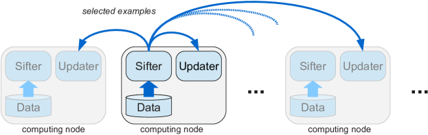
The algorithm operates in two phases, an active filtering phase and a passive updating phase. In the first phase, each node goes over a batch of examples, picking the ones selected by an active learning algorithm using the current model. Model is not updated in this phase. At the end of the phase, the examples selected at all nodes are pooled together and used to update the model in the second phase. The second phase can be implemented either at a central server, or locally at each node if the nodes broadcast the selected examples over the network. Note that at any given point in time all nodes have the same model.
A critical component of this algorithm is the active learning strategy. We use the importance weighted active learning strategy (IWAL) which has several desirable properties: consistency, generality [18], good rates of convergence [21] and efficient implementation [22]. The IWAL approach operates by choosing a not-too-small probability of labeling each example and then flipping a coin to determine whether or not an actual label is asked.
The formal pseudocode is described in Algorithm 1. In the algorithm, we use to denote an active learning algorithm which takes a hypothesis and an unlabeled example set and returns where and is a vector of probabilities with which elements in were subsampled to obtain . We also assume access to a passive learning algorithm which takes as input a collection of labeled importance weighted examples and the current hypothesis, and returns an updated hypothesis.
While the synchronous scheme is easier to understand and implement, it suffers from the drawback that the hypothesis is updated somewhat infrequently. Furthermore, it suffers from the usual synchronization bottleneck, meaning one slow node can drive down the performance of the entire system. Asynchronous algorithms offer a natural solution to address these drawbacks.
Algorithm 2 is an asynchronous version of Algorithm 1. It maintains two queues and at each node . stores the fresh examples from the local stream which haven’t been processed yet, while is the queue of examples selected by the active learner at some node, which need to be used for updating the model. The algorithm always gives higher priority to taking examples from which is crucial to its correct functioning. The communication protocol ensures that examples arrive to for each in the same order. This ensures that models across the nodes agree up to the delays in . See Figure 1 for a pictorial illustration.
2.2 Running time and communication complexity
Consider first an online training algorithm that needs operations to process examples to produce a statistically appropriate model. Apart from this cumulative training complexity, we are also interested in per-example evaluation complexity , which is the time that it takes to evaluate the model on a single example. For instance, the optimization of a linear model using stochastic gradient descent requires operations and produces a model with evaluation complexity independent of the number of training examples, e.g. [23]. In contrast, training a kernel support vector machine produces a model with evaluation complexity and requires at least operations to train (asymptotically, a constant fraction of the examples become support vectors [24]).
Consider now an example selection algorithm that requires operations to process each example and decide whether the example should be passed to the actual online learning algorithm with a suitable importance weight. Let be the total number of selected examples. In various situations, known active learning algorithms can select as little as and yet achieve comparable test set accuracy.
Since we intend to sift the training examples in parallel, each processing node must have access to a fresh copy of the current model. We achieve this with a communication cost that does not depend on the nature of the model, by broadcasting all the selected examples. As shown in Figure 1, each processing node can then run the underlying online learning algorithm on all the selected examples and update its copy of the model. This requires broadcast operations which can be implemented efficiently using basic parallel computing primitives.
| Sequential Passive | Sequential Active | Parallel Active | |
|---|---|---|---|
| Operations | |||
| Time | |||
| Broadcasts |
Figure 2 gives a sense of how the execution time can scale with different strategies. Two speedup opportunities arise when the active learning algorithm selects a number of examples and therefore ensures that . The first speedup opportunity appears when and benefits both the sequential active and parallel active strategies. For instance, kernel support vector machines benefit from this speedup opportunity because , but neural networks do not because . The second opportunity results from the parallelization of the sifting phase. This speedup is easier to grasp when as is the case for both kernel support vector machines and neural networks. One needs computing nodes to ensure that the sifting phase does not dominate the training time. In other words, the parallel speedup is limited by both the number of computing nodes and the active learning sampling rate.
3 Active learning with delays
In most standard active learning algorithms, the model is updated as soon as a new example is selected before moving on to the remaining examples. Both generalization error and label complexity are typically analyzed in this setting. However, in the synchronous Algorithm 1, there can be a delay of as many as examples ( examples on each node) between an example selection and the model update. Similarly, communication delays in the asynchronous Algorithm 2 lead to small variable delays in updating the model. Such delays could hurt the performance of an active learner. In this section we demonstrate that this impact is negligible for the particular importance weighted active learning scheme of Beygelzimer et al. [20]. While we only analyze this specific case, it is plausible that the performance impact is also negligible for other online selective sampling strategies [25, 26].
We now analyze the importance weighted active learning (IWAL) approach using the querying strategy of Beygelzimer et al. [21] in a setting with delayed updates. At a high level, we establish identical generalization error bounds and show that there is no substantial degradation of the label complexity analysis as long as the delays are not too large. We start with the simple setting where the delays are fixed. Given a time , will be used to denote the delay until which the labelled examples are available to the learner. Hence corresponds to standard active learning.
Algorithm 3 formally describes the IWAL with delays. Following Beygelzimer et al. [21], we let be a tuning parameter, while we set and . The algorithm uses the empirical importance weighted error of hypothesis on all examples up to (and including) the example . Formally, we define
where is an indicator of whether we queried the label on example , is the probability of being one conditioned on everything up to example , and is the indicator function.
| (1) |
3.1 Generalization error bound
We start with a generalization error bound. It turns out that the theorem of Beygelzimer et al. [21] applies without major changes to the delayed setting, even though that is not immediately apparent. The main steps of the proof are described in Appendix A. For convenience, define . The bound for IWAL with delayed updates takes the following form:
Theorem 1.
For each time , with probability at least we have
In particular, the excess risk satisfies
It is easily seen that the theorem matches the previous case of standard active learning by setting for all . More interestingly, suppose the delays are bounded by . Then it is easy to see that . Hence we obtain the following corollary in this special case with probability at least
| (2) |
As an example, the bounded delay scenario corresponds to a setting where we go over examples in batches of size , updating the model after we have collected query candidates over a full batch. In this case, the delay at an example is at most .
It is also easy to consider the setting of random delays that are bounded with high probability. Specifically, assume that we have a random delay process that satisfies:
| (3) |
for some constant . Then it is easy to see that with probability at least ,
| (4) |
Of course, it is conceivable that tighter bounds can be obtained by considering the precise distribution of delays rather than just a high probability upper bound.
3.2 Label complexity
We next analyze the query complexity. Again, results of [21] can be adapted to the delayed setting. Before stating the label complexity bound we need to introduce the notion of disagreement coefficient [27] of a hypothesis space under a data distribution which characterizes the feasibility of active learning. The disagreement coefficient is defined as
where
The following theorem bounds the query complexity of Algorithm 3. It is a consequence of Lemma 3 in Appendix B (based on a similar result of [21]):
Theorem 2.
With probability at least , the expected number of label queries by Algorithm 3 after iterations is at most
Once again, we can obtain direct corollaries in the case of deterministic and random bounded delays. In the case of delays bounded determinsitically by , we obtain the natural result that with the probability at least , the query complexity of Algorithm 3 is at most
For a random delay process satisfying (3) the query complexity is bounded with probability at least by
4 Experiments
In this section we carry out an empirical evaluation of Algorithm 1.
Dataset In order to experiment with sufficiently large number of training examples, we report results using the dataset developed by Loosli et al. [28]. Each example in this dataset is a image generated by applying elastic deformations to the MNIST training examples. The first 8.1 million examples of this dataset, henceforth MNIST8M, are available online.111http://leon.bottou.org/publications/djvu/loosli-2006.djvu
Active sifting Our active learning used margin-based querying [29, 30], which is applicable to classifiers producing real-valued scores whose sign predicts the target class. Larger absolute values (larger margins) correspond to larger confidence. A training point is queried with probability:
| (5) |
where is the total number of examples seen so far (including those not selected by the active learner). In parallel active learning, is the cumulative number of examples seen by the cluster until the beginning of the latest sift phase. The motivation behind this strategy is that in low-noise settings, we expect the uncertainty in our predictions to shrink at a rate (or more generally if is the Bayes risk). Hence we aim to select examples where we have uncertainty in our predictions, with the aggressiveness of our strategy modulated by the constant .
Parallel simulation In our experiments we simulate the performance of Algorithm 1 deployed in a parallel environment. The algorithm is warmstarted with a model trained on a small subset of examples. We split a global batch into portions of and simulate the sifting phase of each node in turn. The queries collected across all nodes in one round are then used to update the model. We measure the time elapsed in the sifting phase and use the largest time across all nodes for each round. We also add the model updating time in each round and the initial warmstart time. This simulation ignores communication overhead. However, because of the batched processing, which allows pipelined broadcasts of all queried examples, we expect that the communication will be dominated by sifting and updating times.
Support vector machine The first learning algorithm we implemented in our framework is kernel SVMs with an RBF kernel. The kernel was applied to pixel vectors, transformed to lie in following Loosli et al. [28]. For passive learning of SVMs, we used the LASVM algorithm of Bordes et al. [19] with 2 reprocess steps after each new datapoint to minimize the standard SVM objective in an online fashion. The algorithm was previously successfully successfully used on the MNIST8M data, albeit with a different active learning strategy [19]. The algorithm was modified to handle importance-weighted queries.
For active learning, we obtain the query probabilities from the rule (5), which is then used to obtain importance weighted examples to pass to LASVM. The importance weight on an example corresponds to a scaling on the upper bound of the box constraint of the corresponding dual parameter and yields instead of the usual where is the trade-off parameter for SVMs. We found that a very large importance weight can cause instability with the LASVM update rule, and hence we constrained the change in for any example during a process or a reprocess step to be at most . This alteration potentially slows the optimization but leaves the objective unchanged.
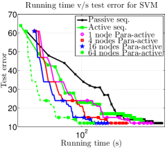
We now present our evaluation on the task of distinguishing between the pair of digits from the pair . This is expected to be a hard problem. We set the global batch size to nearly 4 000 examples, and the initial warmstart of Algorithm 1 is also trained on approximately 4K examples. The errors reported are MNIST test errors out of a test set of 4065 examples for this task. For all the variants, we use the SVM trade-off parameter . The kernel bandwidth is set to , where . We ran three variants of the algorithm: sequential passive, sequential active and parallel active with a varying number of nodes. For sequential active learning, we used in the rule (5) which led to the best performance, while we used a more aggressive in the parallel setup.
Figure 3 (left) shows how the test error of these variants decreases as a function of running time. The running times were measured for the parallel approach as described earlier. At a high level, we observe that the parallel approach shows impressive gains over both sequential active and passive learning. In fact, we observe in this case that sequential active learning does not provide substantial speedups over sequential passive learning, when one aims for a high accuracy, but the parallel approach enjoys impressive speedups up to 64 nodes. In order to study the effect of delayed updates from Section 3, we also ran the “parallel simulation” for , which corresponds to active learning with updates performed after batches of examples. Somewhat surprisingly, this outperformed the strategy of updating at each example, at least for high accuracies.
 |
 |
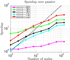
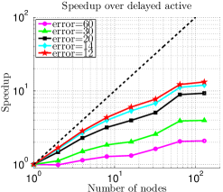
To better visualize the gains of parallelization, we plot the speedups of our parallel implementation over passive learning, and single node active learning with batch-delayed updates (since that performed better than updating at each example). The results are shown in Figure 4. We show the speedups at several different levels of test errors (out of 4065 test examples). Observe that the speedups increase as we get to smaller test errors, which is expected since the SVM model becomes larger over time (increasing the cost of active filtering) and the sampling rate decreases. We obtain substantial speedups until 64 nodes, but they diminish in going from 64 to 128 nodes. This is consistent with our high-level reasoning of Figure 2. On this dataset, we found a subsampling rate of about for our querying strategy which implies that parallelization over 50 nodes is ideal.
 |
 |
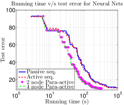
Neural network With the goal of demonstrating that our parallel active learning approach can be applied to non-convex problem classes as well, we considered the example of neural networks with one hidden layer. We implemented a neural network with 100 hidden nodes, using sigmoidal activation on the hidden nodes. We used a linear activation and logistic loss at the output node. The inputs to the network were raw pixel features, scaled to lie in . The classification task used in this case was 3 vs. 5. We trained the neural network using stochastic gradient descent with adaptive updates [31, 32]. We used a stepsize of 0.07 in our experiments, with the constant in the rule (5) set to 0.0005. This results in more samples than the SVM experiments. Given the modest subsampling rates (we were still sampling at 40% when we flattened out at 10 mistakes, eventually reaching 9 mistakes), and because the updates are constant-time (and hence the same cost as filtering), we expect a much less spectacular performance gain. Indeed, this is reflected in our plots of Figure 3 (right). While we do see a substantial gain in going from 1 to 2 nodes, the gains are modest beyond that as predicted by the 40% sampling. A better update rule (which allows more subsampling) or a better subsampling rule are required for better performance.
5 Conclusion
We have presented a generic strategy to design parallel learning algorithms by leveraging the ideas and the mathematics of active learning. We have shown that this strategy is effective because the search for informative examples is highly parallelizable and remains effective when the sifting process relies on slightly outdated models. This approach is particularly attractive to train nonlinear models because few effective parallel learning algorithms are available for such models. We have presented both theoretical and experimental results demonstrating that parallel active learning is sound and effective. We expect similar gains to hold in practice for all problems and algorithms for which active learning has been shown to work.
References
- [1] C. Hui Teo, A. J. Smola, S. V. N. Vishwanathan, and Q. V. Le. A scalable modular convex solver for regularized risk minimization. In KDD, pages 727–736, 2007.
- [2] B. Recht, C. Re, S. Wright, and F. Niu. Hogwild: A lock-free approach to parallelizing stochastic gradient descent. In NIPS. 2011.
- [3] S. Boyd, N. Parikh, E. Chu, B. Peleato, and J. Eckstein. Distributed optimization and statistical learning via the alternating direction method of multipliers. Found. Trends Mach. Learn., 3(1):1–122, 2011.
- [4] J. Langford, A. Smola, and M. Zinkevich. Slow learners are fast. In Advances in Neural Information Processing Systems 22, pages 2331–2339, 2009.
- [5] O. Dekel, R. Gilad-Bachrach, O. Shamir, and L. Xiao. Optimal distributed online prediction using mini-batches. ICML, 2011.
- [6] A. Agarwal and J. C. Duchi. Distributed delayed stochastic optimization. NIPS, 2011.
- [7] A. Agarwal, O. Chapelle, M. Dudík, and J. Langford. A reliable effective terascale linear learning system. CoRR, abs/1110.4198, 2011.
- [8] R. T. McDonald, K. Hall, and G. Mann. Distributed training strategies for the structured perceptron. In HLT-NAACL, pages 456–464, 2010.
- [9] M. Zinkevich, M. Weimer, A. J. Smola, and L. Li. Parallelized stochastic gradient descent. In NIPS. 2010.
- [10] Y. Zhang, J. Duchi, and M. Wainwright. Communication-efficient algorithms for statistical optimization. In NIPS. 2012.
- [11] Y. Zhang, J. Duchi, and M. Wainwright. Divide and conquer kernel ridge regression. In COLT, 2013.
- [12] M.-F. Balcan, A. Blum, S. Fine, and Y. Mansour. Distributed learning, communication complexity and privacy. Journal of Machine Learning Research - Proceedings Track, 23:26.1–26.22, 2012.
- [13] H. Daumé III, J. M. Phillips, A. Saha, and S. Venkatasubramanian. Efficient protocols for distributed classification and optimization. In ALT, 2012.
- [14] H. Daumé III, J. M. Phillips, A. Saha, and S. Venkatasubramanian. Protocols for learning classifiers on distributed data. AISTATS, 2012.
- [15] D. J. C. MacKay. Information based objective functions for active data selection. Neural Computation, 4(4):589–603, 1992.
- [16] D. Cohn, L. Atlas, and R. Ladner. Training connectionist networks with queries and selective sampling. In NIPS, 1990.
- [17] V. V. Fedorov. Theory of Optimal Experiments. Academic Press, New York, 1972.
- [18] A. Beygelzimer, S. Dasgupta, and J. Langford. Importance weighted active learning. In ICML, 2009.
- [19] A. Bordes, S. Ertekin, J. Weston, and L. Bottou. Fast kernel classifiers with online and active learning. Journal of Machine Learning Research, 6:1579–1619, September 2005.
- [20] A. Beygelzimer, D. Hsu, J. Langford, and T. Zhang. Agnostic active learning without constraints. In NIPS, 2010.
- [21] A. Beygelzimer, D. Hsu, J. Langford, and T. Zhang. Agnostic active learning without constraints. In NIPS, 2010.
- [22] N. Karampatziakis and J. Langford. Online importance weight aware updates. In UAI, pages 392–399, 2011.
- [23] L. Bottou. Large-scale machine learning with stochastic gradient descent. In COMPSTAT’2010, pages 177–187, 2010.
- [24] I. Steinwart. Sparseness of support vector machines—some asymptotically sharp bounds. In NIPS. 2004.
- [25] N. Cesa-Bianchi, C. Gentile, and F. Orabona. Robust bounds for classification via selective sampling. In ICML, pages 121–128, 2009.
- [26] F. Orabona and N. Cesa-Bianchi. Better algorithms for selective sampling. In ICML, pages 433–440, 2011.
- [27] S. Hanneke. A bound on the label complexity of agnostic active learning. In ICML, pages 353–360, 2007.
- [28] G. Loosli, S. Canu, and L. Bottou. Training invariant support vector machines using selective sampling. In Large Scale Kernel Machines. 2007.
- [29] S. Tong and D. Koller. Support vector machine active learning with applications to text classification. Journal of Machine Learning Research, 2:45–66, 2001.
- [30] M.-F. Balcan, A. Z. Broder, and T. Zhang. Margin based active learning. In COLT, pages 35–50, 2007.
- [31] J. Duchi, E. Hazan, and Y. Singer. Adaptive subgradient methods for online learning and stochastic optimization. Journal of Machine Learning Research, 12:2121–2159, 2010.
- [32] H. B. McMahan and M. Streeter. Adaptive bound optimization for online convex optimization. In COLT, 2010.
Appendix A Generalization bounds for delayed IWAL
In this section we provide generalization error analysis of Algorithm 3, by showing how to adjust proofs of Beygelzimer et al. [21]. To simplify notation, we will use the shorthand . We start by noting that Lemma 1 of [21] still applies in our case, assuming we can establish the desired lower bound on the query probabilities. This forms the starting point of our reasoning.
In order to state the first lemma, we define the additional notation to refer to the set of triples for . Here, is feature vector, is an indicator of whether the label was queried, and the label is only included on the rounds where a query was made. These samples summarize the history of the algorithm up to the time and are used to train . Recall that .
In the following we let be the error estimated gap between the preferred hypothesis at timestep and the best hypothesis choosing the other label. We also let be the probability of sampling a label when is observed after history is observed.
We start with a direct analogue of Lemma 1 of Beygelzimer et al. [21].
Lemma 1 (Beygelzimer et al. [21]).
Pick any and for all define
| (6) |
Suppose that the bound is satisfied for all and all . Then with probability at least we have for all and all ,
| (7) |
where .
In order to apply the lemma, we need the following analogue of Lemma 2 of [21].
Lemma 2.
The rejection threshold of Algorithm 3 satisfies for all and all .
Proof.
The proof is identical to that of [21], essentially up to replacing with appropriate values of . We proceed by induction like their lemma. The claim for is trivial since the . Now we assume the inductive hypothesis that for all .
Note that we can assume that . If not, then and the claim at time follows from the inductive hypothesis. If not, then the probability for any is based on the error difference . Following their argument and the definition of Algorithm 3, one needs to only worry about the case where . Furthermore, by the inductive hypothesis we have the upper bound . Mimicking their argument from hereon results in the following lower bound on the query probability
Recall our earlier condition that . Hence we have
Combining the above two results yields the statement of the lemma. ∎
Theorem 1.
For each time , with probability at least we have
In particular, the excess risk satisfies
Proof of Theorem 1.
In order to establish the statement of the theorem from Lemma 1, we just need to control the minimum probability over the points misclassified relative to , . In order to do so, we observe that the proof of Theorem 2 in [21] only relies on the fact that query probabilities are set based on an equation of the form (1). Specifically, their proof establishes that assuming we have for the same sequence coming from Lemma 1, then the statement of the theorem holds. Since this is exactly our setting, the proof applies unchanged yielding the desired theorem statement. ∎
Appendix B Label complexity lemma
In this section we derive a natural generalization of the key lemma [21] for bounding the query complexity.
Lemma 3.
Assume the bounds from Equation 7 hold for all and . For any ,
Proof.
The proof of this lemma carries over unchanged from Beygelzimer et al. [21]. A careful inspection of their proof shows that they only require defined in Equation 6 with query probabilities chosen as in Equation 1. Furthermore, we need the statements of Lemma 1 and Theorem 1 to hold with the same setting of . Apart from this, we only need the sequence to be monotone non-increasing, and to be defined based on samples . Since all these are satisfied in our case with appropriately redefined to , we obtain the statement of the lemma by appealing to the proof of [21]. ∎