(Re)partitioning for stream-enabled computation
Abstract
Partitioning an input graph over a set of workers is a complex operation. Objectives are twofold: split the work evenly, so that every worker gets an equal share, and minimize edge cut to achieve a good work locality (i.e. workers can work independently). Partitioning a graph accessible from memory is a notorious NP-complete problem. Motivated by the regain of interest for the stream processing paradigm (where nodes and edges arrive as a flow to the datacenter), we propose in this paper a stream-enabled graph partitioning system that constantly seeks an optimum between those two objectives. We first expose the hardness of partitioning using classic and static methods; we then exhibit the cut versus load balancing tradeoff, from an application point of view.
With this tradeoff in mind, our approach translates the online partitioning problem into a standard optimization problem. A greedy algorithm handles the stream of incoming graph updates while optimizations are triggered on demand to improve upon the greedy decisions. Using simulations, we show that this approach is very efficient, turning a basic optimization strategy such as hill climbing into an online partitioning solution that compares favorably to literature’s recent stream partitioning solutions.
Index Terms:
Graph-partitioning, Stream Processing, Load Balancing, Network Cuts.I Introduction
Contemporary big-data applications ingest considerable amounts of data to produce meaningful and valuable information. As datasets keep on growing to unprecedented sizes, applications must rely on efficient and scalable computation means. Graph-based applications as social networks [1], search engines or recommender systems [2] have to deal with giant and constantly evolving networks of user or item interactions. As those terabytes of data cannot be efficiently processed and served by a single machine in the horizontal scalability model using commodity hardware, the solution is to partition the interaction graph onto multiples machines for parallel computation and request handling [3]. As computation is fast with this scheme, the dataset evolution could be incorporated seamlessly by the application, so that fresh results are always available.
The MapReduce framework allows to process massive amount of information, in an offline manner [4]. Since very recently, there is a resurgence of interest about stream processing, with the proposal of open platforms such as Storm [5] or commercial ones like Google MillWheel [6] or Amazon Kinesis [7]. In this framework, data is treated as a flow, and each flow element is processed on the fly (and then possibly discarded). While more restrictive that MapReduce, this allows for online computation.
As the raison d’être of stream processing is to exhibit a low latency in its operation, relying on offline partitioning methods is not an option. As the graph structure continuously changes due to node/edge creations, calling a procedure that recomputes a partitioning from scratch at each change is overkill (see e.g. traditional approaches as [8]). In other words, incremental approaches to partitioning are mandatory. In this light, datacenter applications like Pregel [9] partition nodes onto machines based solely on their IDs; this is apparented to dispatch those nodes at random. A recent work proposes to load the graph stored on a disk as a stream of nodes, and to use cheap heuristics for node placement over one of the processing machines on the fly [3]. Although the fact that this approach handles nodes as they are read, it assumes a full knowledge model, where the whole graph is accessible at a given time as the input.
In this paper, we propose a system that receives incoming edges, and places their endpoint nodes greedily in partitions, then performing online partitioning. Our system operates over a continuous flow of events arriving at a datacenter, then suiting the stream processing paradigm. Greedy placement is complemented with periodic partitioning reconfigurations at runtime, using solely little feedback from the application.
The contributions of this paper are:
-
•
to exhibit (i) the instability of optimal partitions created by static partitioning algorithms, if they are run each time few new edges are added to the current graph, and (ii) the existence of a graph-related tradeoff between a well balanced graph (work is evenly divided among the parallel instances) and a low edge cut (workers should be able to process most of the requests using information local to their partition). Intuitively, this tradeoff pops up every time the system has to decide between favoring edge-cut at the price of well balancedness, or vice versa.
-
•
based on these observations, to consider the problem of stream-enabled graph partitioning as a standard mathematical optimization problem. In this problem, the optimization parameters are the well balancedness and the edge-cut, and the metric to optimize is the application performance, measured for instance by the average request processing time.
-
•
to propose a stream-enabled graph partitioner built upon these observations. The realistic simulations we conducted show that a standard greedy optimization is efficient compared to current state-of-the-art stream-enabled partitioner [3], while executing in a more restricted model. Thanks to the greedy nature of the optimization, this performance is achieved for cheap.
The remaining of this paper is structured as follows: Section II exhibits the danger of seeking optimal partitionings in the context of streamed graphs, before presenting the model of execution considered. We then observe in Section III that traditional graph partitioning metrics are bound by a graph-dependent tradeoff that impacts application performance. Based on these observations, Section IV models the streamed-graph partitioning problem as an optimization problem, and proposes a greedy online partitioning mechanism, along with simulation results. A reconfiguration technique to be used periodically at runtime is then presented. Section V illustrates this partitioning scheme in an application context: graph-based recommendation. We finally present Related Work in Section VI before we conclude.
II Model: processing over streamed graphs
II-A Instability of Optimal Partitionings
This sections illustrates the difficulty of simply transposing traditional graph partitioning metrics in the context of graph streaming. The first major problem comes from the complexity of finding an optimal partitioning, which is NP-complete [10]. Considering the update rate of a streamed graph, such problem would have to be solved for every increment, which is not realistic.
Second problem stems from the unstability of such optimal partitioning. To illustrate this, consider the following example. Assume that servers operate on a graph composed of a ring of fully-connected clusters , with . Assume for , we have links between and , and links between and , with . Figure 1 illustrates such topology in the case .

Since any graph partition cutting through a cluster would cut at least links, balanced cuts are either along , either along . Assume : the optimal assignment is to map to server . Now assume that two new edges arrive on the cut, for instance between and . The new optimal assignment is to map to server . To reach this new optimal assignment, nodes need to be transferred during the reconfiguration. Observe that the arrival of two new edges along a cut (or the removal of two edges along an cut) can now generate the same amount of reconfigurations.
Let us imagine a worst case scenario where originally and , and a stream of edges repeating the aforementioned scheme () until . The described reconfiguration then happens times. This implies node transfers. Although this is a pathological worst-case scenario, bad situations cannot be discarded in dealing with real world graphs either. This illustrates the need for a specific approach to support graph updates, then adapted to the streamed graph model we now define.
II-B Partitioning Model and Metrics for Streamed Graphs
We consider a streamed graph model, where edges arrive continuously to a central machine called the partitioner, . is in charge of partitioning the streamed graph over a fixed set of machines or cores, according to the computing hardware setup. Practically, it positions an incoming edge endpoints (i.e. nodes) on one or two of the machines that are hosting a partition of , under the form of adjacency lists. can be seen as the graph resulting from the aggregation of all arrivals, at the end of times. denotes partition number , and the number of nodes currently in . Each partition has the capacity to host nodes. then contains all nodes and edges from seen so far.
We do not make any assumption on the order of arrival of elements in set . The system operates on edges, implying that if one endpoint (i.e. one node) is unknown, its creation is handled by the system. denotes the set of neighbors of node .
maintains a table mapping all nodes seen so far (i.e. edge endpoints) to their current partition assignment (an integer ), for being able to take greedy decisions on placement of incoming edges. State maintained at is thus .
In this paper, we are interested in optimizing the average request processing time of the application on top of which our partitioning system is deployed. However, throughout the paper, we refer to two traditional metrics of graph partitioning:
-
•
Load balancing is computed as the spread between the less and the more loaded of the partitions. It can be written as
where 0 denotes a very uneven load between the partitions, and 1 denotes a perfect balancing.
-
•
Cut is the fraction of edges that have endpoints located in different partitions. This represents an important quantity, as traversing such edge will require data to be exchanged among the machines, therefore adding latency to the request processing time. Formally, the cut is defined as:
Again, 0 denotes a non-desirable situation where all edges have endpoints in different partitions, and 1 denotes a partitioning cutting no edge.
III Partitioning: cuts, load and applications
Let us first consider a coarse model of the environment of an application running in a centralized setting. Upon arrival of a request , this application will consume two quantities: memory and CPU time. Let and be these quantities. In this abstract model, we consider that the system knows instantly at the arrival of what will be and .
The system is able to provide memory and processing power at rate and per time unit, respectively. Therefore, if is the only request on the system, we consider that its processing will take the time required to gather the required resources . As a simple model for congestion, assume that requests are processed on the system at each time. Then becomes : the system evenly splits its processor and memory supply to all the requests, and side effects (such as context switch) are neglected.
Now let us consider the same application running in a distributed setting. The input of this application is a graph : the memory requirements of a request can now be expressed as a subgraph of : . We consider the following distributed setting: machines are fully connected through synchronous equal links. Each machine has enough memory to hold a subgraph such that forms a partition of .
III-A Analyzing a Simple Locality Model
Let us assume the memory needs of a request consist in the -hop neighborhood of a node: , where is the center of request . We define as a measure of requests’ locality. Let us illustrate this concept:
-
•
the request “get ’s neighbors” has a locality of : the neighbors of are known locally by .
-
•
the request “get ’s eccentricity” has a locality of , the graph diameter, as the most eccentric nodes are hops apart.
-
•
a damping random walk (jump with a probability ) can be modeled by an “expected” locality (e.g. ).
Let be the machine holding node , center of a request of locality . If , all the required information to process is already available on , the request processing time only depends on the processing resources available on . However, if , then information will have to be fetched from machine , and the duration of this fetch will add up to the request processing time.
More formally, let be the network latency induced by such fetching operation. We consider that remote fetches cannot be made parallely, mostly because in the streaming context the hop neighbors (and therefore the partitions holding them) are not known in advance beside direct neighbors. Therefore we model the processing time of request when processed by as:
Observe that the computing time contribution depends on the size of since the bigger the partition is, the more requests machine will have to serve in parallel. The information gathering time also depends on since the bigger is, the higher the chances are that , therefore reducing the information gathering time to 0.
Thus, we have here a first visible tradeoff the partitioning strategy has to solve in order to minimize request compute time:
-
•
Computations over small partitions are processed faster, since the load on the machine holding the partition is low, at the cost of higher information gathering costs.
-
•
Computation over big partitions are slower, but require on average less information fetching.
Now, considering that we have a fixed number of machines , this tradeoff translates in: shall we prefer to minimize the cut or to optimize the load balancing ?
III-B Graph-Related Tradeoff
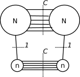
With the aforementioned tradeoff in mind, consider the graph depicted figure 2. This graph consists in fully connected clusters of sizes and . Clusters of equal size are connected by links, and two links connect one cluster of size with one of size . Assume that and . Two key observations are:
Now let us compute the average request processing time centered on a node . Since we have only two clusters, assuming , computing the information fetch cost is easy. Let be the boundary of each cluster, and .
Assume well balancedness is preferred:
| (1) | ||||
| (2) |
Now assume cut minimization strategy is preferred:
| (3) | ||||
| (4) | ||||
| (5) | ||||
| (6) |
If we compare those two quantities we have:
| (7) | |||||
| (8) | |||||
| (9) | |||||
| (10) | |||||
| (11) | |||||
Therefore, in such a setting, one can draw the following conclusions:
-
•
if the problem is only local (), well balancedness is always faster.
-
•
under this last form, the inequality’s left hand side only contains application and hardware dependent variables, that are unlikely to change along the progress of the stream. The inequality’s right hand side only contains graph dependent variables: these are likely to evolve along the streaming progress.
This simple model illustrates a major problem of classical graph-partitioning approaches when dealing with the incremental nature of streamed graphs: the fastest partitioning strategy depends both on the target application and on the target graph. As at least the graph is unknown, meaning that we cannot make strong assumptions on the evolution of its characteristics or on the order on which will be received particular updates, we therefore argue that an online exploration of this well balancedness/min-cut tradeoff is mandatory for top-application performance.
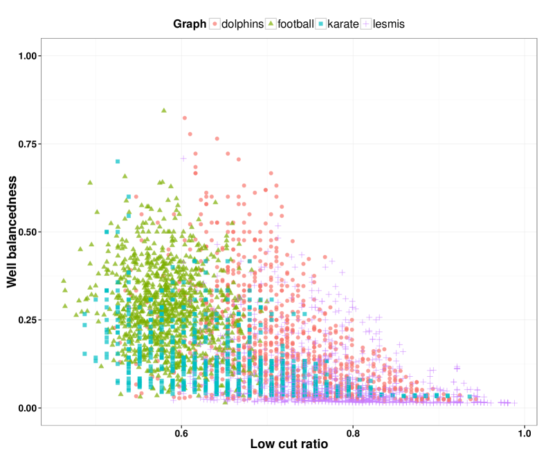
One might wonder, due to the artificial nature of the constructions used to illustrate this tradeoff, whether such situation do happen in practice. To answer this question, we took a set of standard small real-world topologies111Topologies are available at http://www-personal.umich.edu/~mejn/netdata/. The authors would like to thank M.E.J. Newman for providing these topologies., and randomly partitioned them into pieces, and measured the obtained well balancedness and cut size. We repeat the process times for each topology, therefore “sampling” the partitioning configuration possibilities. Figure 3 represents the obtained results. Each point represents a random partitioning, and although chances are low that optimal partitionings are represented on this figure, the point cloud associated with each topology represents the likely outcomes of partitionings. As we can see, they differ from one topology to the other: each topology allows its own tradeoff between well balancedness and low edge cut.
IV (Re)partitioning from streamed graphs
We have seen in previous sections that the hardness of partitioning precludes a new partitioning iteration on the whole graph at each new edge arrival. We have established that the partitioning achieving the lowest request processing time has to find an optimum between a good load balancing, and a low edge cut. Moreover, we have seen that such optimum not only depends on the application, but also on the characteristics of the streamed graph.
We now propose a greedy solution for partitioning and reconfiguration, that handles increments as graphs are streamed.
IV-A Global Framework Overview
The framework we propose is the following one, as shown on Figure 4. The stream of incoming graph updates (edge additions) is dispatched to the partitions by . Since the optimal balance between load balanced partitions and low cut ratio depends on the graph (which is constantly evolving) and the application (whose sweet spot for performance is not necessarily known), and since the continuous stream of updates has to be handled as quickly a possible, the partitioner decides which partition to assign new edges to in a greedy fashion. A logical optimizer monitors the state of the machines, and periodically optimizes this greedy layout by choosing nodes in partitions, and by migrating them. The choice of which nodes to move, and of where to migrate them is driven by an optimization procedure following two strategies: it tries to improve either the edge cut, either the load balancing. The precise role of each component is described afterwards.
IV-B Stream-greedy: A Simple Greedy Partitioner
We first introduce the two related work competitors for efficient online partitioning.
IV-B1 Related Approaches
The common approach, due to its simplicity, is to partition at random. Once a node arrives at the datacenter, a partition is selected according to a modulo operation over the node identifier (itself being pseudo-random), see e.g. Pregel [9]. This often called hashing.
More advanced heuristics for partitioning a graph that is read from disk as a stream of nodes, are presented in [3]. They all outperform hashing. The best performing heuristic is called weighted deterministic greedy, and is node driven. It consists of placing an incoming node to the partition where it has the most edges, weighting this by a linear penalty function based on the capacity of the partition:
| (12) |
All methods stream nodes in random order or in a breadth/depth first search fashion. The major assumption of this technique is that each streamed node comes with its complete (non-yet seen) neighbor-list. This make this study not applicable to the stream processing model where edges are received as events at a datacenter along the application life (as opposed to nodes read from a disk containing the whole graph).
We pick this deterministic greedy heuristic as the baseline technique to compare to in the rest of this paper.
IV-B2 stream-greedy partitioner
As we are bound to a restrictive model where edges are received arbitrarily following the application logic, and because a crucial point for system scalability is to propose a fast and lightweight partitioning method at , we detail a simple and intuitive greedy partitioner: when arrives at the datacenter, placement decision is made following the pseudo-code provided on Algorithm 1. is a function triggered by , that informs machines hosting and (they could be one single machine) to link those two nodes via an edge in their respective adjacency lists.
Computationally, this heuristic simply requires to perform membership tests and cardinality operations over the mapping table (for finding the least represented partition).
IV-C Improving Current Partitioning
To improve the current partitioning, the optimizer relies on two heuristics. The first targets an improvement on the load balancing criterion, while the second targets an improvement on the cut criterion. The simulation results presented Section IV-D show that both heuristics are efficient most of the time: each one improves one metric without significant degradation of the other.
Both heuristics select nodes from machines based on their “badness”, which measures each node’s individual contribution to the size of the cut. Rationale behind using the same selection being that even if load balancing is not concerned by cut ratio, selecting bad nodes instead of random ones does not degrade intentionally the second metric. For each node in a partition , it is formally defined as:
| (13) |
(the lower the worse). However, while improvement towards cut selects the same amount of nodes in each machine, the load-balancing improvement heuristic only selects nodes on the most loaded machines.
The selected nodes are then migrated to a different machine. Again, heuristic improving cut proceeds while ignoring actual load on the machines: it migrates each selected node to the partition containing the most of its neighbors:
| (14) |
In contrast, the load balancing heuristic takes each machine load into account when selecting a new partition for each node: for this it relies on the baseline strategy (12). Note that we can apply baseline, as when this heuristic is executed, the system deals with already received edges and nodes for reconfiguration.
Afterwards, both heuristics proceed the same way. They send the node to the selected partition, and update regarding the node’s new location.
Given the state of the partitioning at a given time, improving on one criterion means reconfiguring the system, by moving a small part of system nodes from one partition to another one. The migration rate must be small, in order not to impact the application running on top of the partitioning. The optimizer measures the application performance at runtime, decides when to reconfigure, chooses a reconfiguration strategy, and commits it if it considers this reconfiguration was successful. In order not to force the developers to over instrument the application, and for overall simplicity/reusability, we built a system that self-tunes solely based on one information given by the application at runtime. This information takes the form of the average computation time. From this value, the optimizer decides when to trigger a reconfiguration, and measures after a reconfiguration if the average runtime is lower or not than before a reconfiguration.
The optimization problem is then to reach a configuration, i.e. a certain graph partitioning, that minimizes request execution time at the application level. As finding a particular graph partitioning is NP-complete (e.g. bisecting static graphs [10]), we have to rely on local search optimization. Considering our computing time feedback, and two improvement criterions, a natural optimization framework is hill climbing. The difference of our setup with canonical hill climbing is that we cannot instantly evaluate both neighbors of current configuration, i.e. the new configuration after a step on load balancing and after a step on cut ratio. We thus make a random choice towards one criterion, and act as a function of resulting computing time. We call this variant blind hill climbing.
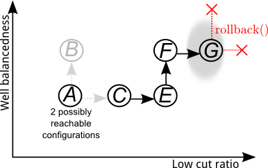
This approach is summed-up by Figure 5; periodic optimizations are conduced under trial and error. When no progress is possible in any of the two directions, the configuration has reached a sweet spot for the application performances. Note that as nodes and edges arrive continuously at the datacenter, this spot moves after each addition. Each optimization step then performs in best effort fashion voluntarily considering current graph as static.
Finally, note that we presented the optimizer as an independent centralized entity for the sake of clarity. In practice, the optimizer task is distributed on the set of machines hosting partitions.
IV-D Simulation Results
IV-D1 Simulation Setup
For the sake of comparison with simulation results conduced in [3], we use the same three graphs depicted as representative from the major three types of network structures. The first one, PL1000, is a synthetic graph of nodes with clustered power-law characteristics222generated with NetworkX (http://networkx.github.io/). The social network, Marvel, consists in characters, having interactions in comics. The last graph, 4elt, of nodes and edges, is a FEM graph from the NASA.
For all three datasets, as the graph is streamed in a random order from the first edge to the last one. The number of partitions is set to for PL1000, for Marvel and for 4elt, as in [3] for matters of reproducibility. Our greedy heuristic, as well as random and baseline results are exposed. Please note that as baseline assumes that when a node arrives at the partitioner, all its (future) neighbor nodes are also known, we implement such assumption in our simulation. This clearly gives it an advantage over the two other approaches, but also serves as an indicator of the gap between our greedy method and the one with full knowledge.
IV-D2 stream-greedy performance
We now assess the performances of random, baseline and stream-greedy heuristics by simulation, in a streamed graph setup.
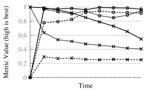
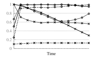
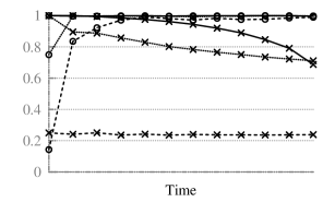
Figure 6 present results for well balancedness (lines with rounds) and cut (lines with crosses) metrics on the y-axis, the higher the better. The x-axis represents time, from where first edge is dispatched, to where the whole graph has been streamed (then having partitioned).
Regarding load balancing curves, results for all three graphs and all three competitors are consistent and close to perfect balancing at , and all three are comparable. Now regarding cut, we first remark that baseline results are consistent with results produced in [3] (where only cut ratio is considered), as operating under the same assumptions. Produced results for random partitioning are also consistent with theory, as random placement is awaited to cut a fraction of of edges, thus for and for . The first learning is that baseline always beats random partitioning (as seen in [3]); this is also the case for our greedy approach. Surprisingly, despite the fact that baseline beats stream-greedy on Marvel and slightly on 4elt graphs, stream-greedy outperforms the deterministic greedy approach on PL1000. This shows that even with an increased amount of information, baseline does not perform better, as it could be beaten by stream-greedy, even operating on less information. We thus learn that operating under reduced assumptions still make possible a very competitive first partitioning step, using an intuitive partitioner such as stream-greedy.
We have presented and compared a simple one pass greedy stream partitioner; as a consequence, edges placed by that heuristic are never moved from one partition to another one. Next section shows that we can periodically improve on one criterion or the other at runtime.
IV-D3 Improving on Cut Ratio
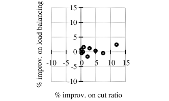
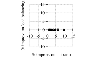
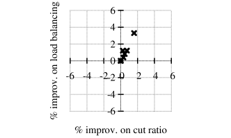
Figure 7 presents improvement percentages for the cut criterion. Ideally, running a heuristic on one criterion (e.g. on cut ratio) should of course improve it, but also avoid degrading the second one (e.g. not degrade load balancing). Simulations show that, on the same three graphs at , there is room for improvement. With a typical value for top- worst nodes of , up to improvement is achieved at each procedure call, after what next calls produce more slight changes. We also see that except for few percent on the Marvel graph, improving on cut ratio does not degrade current load balancing of graphs.
IV-D4 Improving on Load Balancing
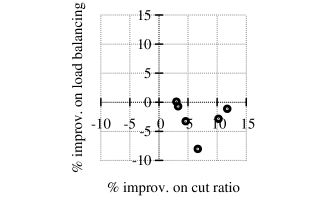
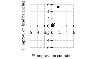
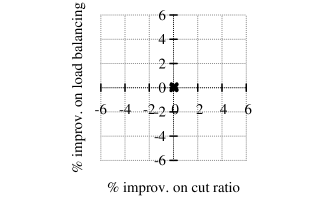
Figure 8 presents results. Improvement on load balancing at each call is positive but less important that for improvement on the cut ratio criterion. This is explained by the fact that at , as seen on Figure 6, load balancing is already close to perfect. Those calls does not degrade the other criterion either.
V Illustration: graph-based instant recommender
We now present a direct application of this optimization framework in a system leveraging streamed graphs, detail implementation needs, and show performance indicators.
V-A System Implementation of Blind Hill Climbing
Regardless of the application relying on the partitioning process, few system primitives are required to implement the optimization framework. Here is a list:
-
•
snapshot(): atomically records node/edge repartition over machines.
-
•
getComputeTime(): top application returns current average compute time.
-
•
commit(): remain in current configuration, and free structure used for snapshoting.
-
•
rollback(): return to previous configuration (snapshoted earlier).
-
•
buffer(): record all incoming events (edges, requests) in a message queue. flushBuffer() consumes those buffered events.
From those primitives, we propose the following heuristic, that pursue a hill climbing optimization based on application feedback (see Algorithm 2).
As configuration switch has practical costs, system parameter denotes the degradation threshold over which it is profitable to rollback to previous configuration. This threshold also masks the slight deviation in average computing time due to particular request patterns, or due to the arrival of nodes and edges in between two optimizations.

V-B A System for Instant Recommendation
A typical example of a latency critical service is recommendation. The reactivity capabilities of the application to process fresh data is key for successful services, as accurate and instant recommendation based on previous clicks for instance [11]. We take the scenario of movie recommendation for the rest of this paper. In this framework, nodes are users/movies and an edge is present if one user has rated a particular movie. We are interested in treating ratings as a stream, as their direct incorporation into the system for instant recommendation can for instance solve the cold start problem at user registration (i.e. before waiting for the platform to compute offline for later personalized recommendations).
Bahmani et al. [2] show that a variant of Pagerank, based on random walks, provides fast and personalized recommendations. On a user/item graph, it essentially consists in launching multiple (damping) random walks from the node (user) that needs a recommendation; most visited nodes (items) are extracted through higher Pagerank values and sorted. On such a graph, top-nodes (items) are good recommendations for that user.
As random walks are locality critical in the context of parallel computing, we expect partitioning to be crucial for the recommender performances. With a good partitioning (high density of links within machines and low edge cut), launched damping random walks stay on the same machine333We prototyped a Storm-based system [5] implementing this recommendation engine, and answering to PUT/GET queries on the MovieLens graph. While adding and edge is made instantly, average computing time for single sequential GET recommendations is around ms (using as much as random walks per recommendation), over a Xeon E5-2603 CPU (DELL T5600). This motivates the will to keep computation local to a machine for both speed and capability to handle many concurrent requests.. If not, then many dependencies arise from inter-machines communications.
V-C Simulation Over the MovieLens Dataset
We ran personalized Pagerank for recommendation over the MovieLens dataset [12], a user/movie graph consisting of ratings from users on movies.
The blind hill climbing optimization, described on Algorithm 2, is implemented by a logical optimizer in the following way. controls the frequency of optimizations. When decides to perform an optimization step, it flips a coin to choose on which criterion to try to improve. It then stops consuming events by calling the buffer() primitive (architecturally this correspond in practice to let the message queue store events, e.g. [13], and let it grow for an instant). Order to call improvement heuristic is broadcasted to the machines. Bad nodes are computed (according to metric (13)) on each machine, in order not to add computational burden onto the partitioner. On this simulation of the worst nodes of each partition are migrated in each optimization cycle. Once optimization has completed on all machines, a generic batch of requests is artificially executed on the system. If getComputeTime() returns a degraded average completion time, the partitioner broadcasts a rollback order (a commit one otherwise). The rollback to previous partitioning configuration is executed in a lockstep at each machine, by a simple memory overwrite from previous snapshot() result. then returns in service mode by calling flushBuffer(). This simple implementation constitutes a coarse grain handling of system states; we leave a finer grain handling of consistency for future work.
The primary metric to assess performance of the application related to a given partitioning is the number of dependencies. A dependency of the application occurs when a random walk (launched at any machine) has to get onto another machine to pursue process. It is a direct indicator of the latency at the application level, as network costs clearly overcome local CPU computation.
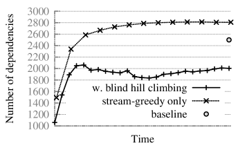
Each simulated request triggers random walks (with a min-hop of away from the querying user, and a damping factor of ). To simulate the increase of application-usage as the graph grows, we ran a number of user requests of times the current graph size, after each increase of the number of edges by . With an optimization step being triggered when graph size increases by , , and , dependencies are plotted on Figure 9(a), as they evolve while the graph is streamed. The hill climbing optimization clearly maintains dependencies at a lower level than stream-greedy (close to less). The static partitioning resulting from baseline performs again slightly better than stream-greedy, but as its operation is not periodically optimized, it cannot compete with our blind hill climbing approach.
We now plot the on Figure 9(b) the success/failure of calls to improvement heuristics. For optimizations on a random criterion, are successful on cut ratio criterion, and on load balancing. There is only rollback on cut, but on load balancing. The more important failure rate over load balancing is due to the already very good balance achieved without optimization, as seen on Figure 6 for other graphs with stream-greedy. A solution to decrease this failure rate is to bias the random choice towards the more successful of the two criterions (i.e. learn and call the most successful one with a higher probability).
In conclusion, there is a clear advantage in periodically reconfiguring current partitioning by calling lightweight optimization procedures, for correcting past greedy decisions in the context of streamed graphs. The framework we propose only takes as input the application feedback and allows self-tuning in an efficient way.
VI Related Work
Static partitioning approaches take a graph as input and propose a bisection as output (known as the minimum bisection problem). Reaching a configuration with minimal number of inter-machine edges while balancing the output is well known to be NP-complete [10]. This as been extended to -partitioning, where the input graph is partitioned into pieces [8]. Methods for partitioning largely depend on the application using the produced partitions, as computing while partitions fit network architecture [14], minimizing interactions between storage servers [1], or computing over embarrassingly parallel datasets [9] for instance.
Approaches like GraphChi [15] or TurboGraph [16] aim at computing metrics over large graphs on a centralized setting; they differ from stream-based approaches as they compute offline over the dataset and do not consider graph updates for low latency operation and online request handling.
Staton et al. [3] are the first to consider a stream of nodes to be placed onto partitions on the fly. Many heuristics are proposed and tested, from intuitive ones (considering balance) to more advanced ones (considering clustering coefficient); we re-implement the best performing one in this paper to compare it to our proposal. All approaches are one pass; a placed vertex is never moved afterward. Their paper assumes a full knowledge model, where the graph to be streamed has to be present on one machine prior to the execution of the proposed heuristics.
VII Conclusion
This paper has exposed the hardness of partitioning a streamed graph not already present on a computing device. A greedy partitioner taking as input stream of edges has been proposed, that can compete with a state of the art heuristic for partitioning under full knowledge. While its operation is satisfying, we show that it is of interest to periodically call an optimization procedure to improve upon current partitioning, on the edge cut ratio or on the load balancing criterions. These building blocks form a general optimization framework allowing for application self-tuning, based solely on feedback on computing time. An interesting question for future work is to formally ask if there exists a greedy algorithm having provable bounds for its efficiency to partition a streamed graph, in the classic stream processing model.
References
- [1] J. M. Pujol, V. Erramilli, G. Siganos, X. Yang, N. Laoutaris, P. Chhabra, and P. Rodriguez, “The little engine(s) that could: scaling online social networks,” IEEE/ACM Trans. Netw., vol. 20, no. 4, pp. 1162–1175, Aug. 2012. [Online]. Available: http://dx.doi.org/10.1109/TNET.2012.2188815
- [2] B. Bahmani, A. Chowdhury, and A. Goel, “Fast incremental and personalized pagerank,” in VLDB, 2010.
- [3] I. Stanton and G. Kliot, “Streaming graph partitioning for large distributed graphs,” in KDD, 2012.
- [4] J. Dean and S. Ghemawat, “Mapreduce: simplified data processing on large clusters,” Commun. ACM, vol. 51, no. 1, pp. 107–113, Jan. 2008. [Online]. Available: http://doi.acm.org/10.1145/1327452.1327492
- [5] N. Marz, “Storm Project,” http://storm-project.net/, 2012.
- [6] T. Akidau, A. Balikov, K. Bekiroglu, S. Chernyak, J. Haberman, R. Lax, S. McVeety, D. Mills, P. Nordstrom, and S. Whittle, “Millwheel: Fault-tolerant stream processing at internet scale,” in VLDB, 2013, pp. 734–746.
- [7] Amazon, “Amazon Kinesis,” http://aws.amazon.com/kinesis/, 2013.
- [8] K. Andreev and H. Räcke, “Balanced graph partitioning,” in SPAA, 2004.
- [9] G. Malewicz, M. H. Austern, A. J. Bik, J. C. Dehnert, I. Horn, N. Leiser, and G. Czajkowski, “Pregel: a system for large-scale graph processing,” in SIGMOD, 2010.
- [10] M. R. Garey and D. S. Johnson, Computers and Intractability; A Guide to the Theory of NP-Completeness. New York, NY, USA: W. H. Freeman & Co., 1990.
- [11] G. Linden, B. Smith, and J. York, “Amazon.com recommendations: Item-to-item collaborative filtering,” IEEE Internet Computing, vol. 7, no. 1, pp. 76–80, Jan. 2003.
- [12] J. L. Herlocker, J. A. Konstan, A. Borchers, and J. Riedl, “An algorithmic framework for performing collaborative filtering,” in SIGIR, 1999.
- [13] B. Cook, “Kestrel distributed message queue,” https://github.com/robey/kestrel/, 2013.
- [14] D. Ajwani, S. Ali, and J. Morrison, “Graph partitioning for reconfigurable topology,” in IPDPS, 2012.
- [15] A. Kyrola, G. Blelloch, and C. Guestrin, “Graphchi: large-scale graph computation on just a pc,” in OSDI, 2012.
- [16] W.-S. Han, S. Lee, K. Park, J.-H. Lee, M.-S. Kim, J. Kim, and H. Yu, “Turbograph: a fast parallel graph engine handling billion-scale graphs in a single pc,” in KDD, 2013.