MCRG Flow for the nonlinear Sigma Model

Abstract:

A study of the renormalization group flow in the three-dimensional nonlinear O(N) sigma model using Monte Carlo Renormalization Group (MCRG) techniques is presented. To achieve this, we combine an improved blockspin transformation with the canonical demon method to determine the flow diagram for a number of different truncations. Systematic errors of the approach are highlighted. Results are discussed with hindsight on the fixed point structure of the model and the corresponding critical exponents. Special emphasis is drawn on the existence of a nontrivial ultraviolet fixed point as required for theories modeling the asymptotic safety scenario of quantum gravity.

1 Asymptotic Safety

In a renormalization group approach to QFT the theory at momentum scale $k$ is described by the effective average action $\Gamma_{k}$. It is obtained by choosing a microscopic action at some cutoff-scale $\Lambda$ where $\Gamma_{\Lambda}=S_{mic}$ and integrating out fluctuations with scales between $\Lambda$ and $k\ll\Lambda$ using the renormalization group flow. We call a theory fundamental if it is valid on all scales, i.e. the limit $\Lambda\rightarrow\infty$ and $k\rightarrow 0$ exists when one fine-tunes only a small number of parameters. For gravity, we know the infrared theory very well - it is given by the Einstein-Hilbert action. However, the perturbative approach to find a formulation that is valid at small distances and high momenta reveals severe divergences: gravity is not renormalizable in a perturbative manner. But it should still be possible to renormalize gravity nonperturbatively at a non-Gaussian ultraviolet fixed point with a finite number of relevant directions (asymptotic safety scenario [2]). In this contribution, we study the nonlinear O(N)-models in $D=3$ dimensions, which are expected to show a nontrivial UV fixed point [3, 4]. The action is

$$S=\frac{1}{2g^{2}}\int d^{3}x\;\partial_{\mu}\vec{\phi}\partial^{\mu}\vec{\phi}\text{, \; with }\vec{\phi}\in\mathbb{R}^{N},\quad\vec{\phi}\vec{\phi}=1.$$ (1)

Our goal is to obtain the global flow diagram from lattice simulations and determine its fixed point structure. To achieve this, we utilize Monte Carlo Renormalization Group (MCRG) techniques.

2 MCRG method

On the lattice, the discrete momenta are cut off by the inverse lattice spacing $a^{-1}$ in the UV and the inverse box length $(aL)^{-1}$ in the IR and a lattice simulation is equivalent to integrating out all fluctuations in between (see figure 1).

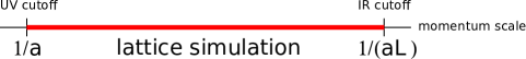
Figure 1: A lattice simulation integrates out all the momenta between the upper cutoff $\Lambda=a^{-1}$ and the lower cutoff $(aL)^{-1}$.

The correlation functions of the theory are determined by direct measurement of lattice operators. By applying a blockspin transformation with scale factor $b$, the upper cutoff is reduced whereas the lower cutoff does not change: $a^{-1}\rightarrow(ba)^{-1}$, $(aL)^{-1}\rightarrow(baL/b)^{-1}=(aL)^{-1}$, see figure 2.

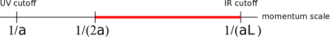
Figure 2: A blockspin transformation with scale factor $2$ reduces the upper cutoff $\Lambda\rightarrow\Lambda^{\prime}=\Lambda/2$, yet leaves the lower cutoff $(aL)^{-1}$ unchanged.

At the reduced cutoff, we define an effective theory such that the IR physics of the original and effective theory coincide, i.e. both theories lie on the same RG trajectory. In the RG picture, we have obtained the effective theory by integrating out the momenta from $a^{-1}$ until $(ba)^{-1}$.
In our setup, we use a local HMC algorithm for the O(N)-valued field to compute a Markov-chain of configurations. This algorithm allows to simulate arbitrary N with high acceptance rate. Also, it is straightforward to add further operators to the action,

$$S[\vec{\phi}]=\sum_{i}g_{i}S_{i}[\vec{\phi}].$$ (2)

On each configuration, we apply a blockspin transformation to integrate out fluctuations and on the blocked configurations, we use the canonical demon method [5] to determine the couplings $g_{i}^{blocked}$ of the effective theory. In this way, we have access to the discrete beta function $\tilde{\beta}_{i}=\tilde{\beta}(g_{i})=g_{i}^{blocked}-g_{i}$ and the discrete stability matrix $S_{ij}=\frac{\partial\tilde{\beta}_{i}}{\partial g_{j}}$. The eigenvalues of the stability matrix in the vicinity of a fixed point can be related to its critical exponents.

3 Systematic errors

After comparing RG trajectories from different lattice sizes, no finite volume effects are visible in our results for the $32^{3}\rightarrow 16^{3}$ simulations. Also, we expect discretisation errors to be small near the critical line, where the correlation length diverges in the continuum limit. However, using an effective action in the demon method inevitably leads to truncation errors. In particular, the semi-group property of the combined transformation $R_{b}$ of blockspin transformation and demon method is violated: $R_{b}\circ R_{b}\neq R_{b^{2}}$. Concerning the RG trajectories, this leads to a discrepancy in the effective couplings of a chain of two transformations, with scale factor $b$ each, compared to a single transformation with scale factor $b^{2}$. In order to minimize this discrepancy we add further operators to the effective action 2 following a derivative expansion. Our best truncation consists of four operators which represent all possible operators of this model up to fourth order in the momenta:

$$S_{0} =-\int d^{3}x\;\vec{\phi}\partial_{\mu}\partial^{\mu}\vec{\phi},$$ (3)

$$S_{1} =-\int d^{3}x\;\vec{\phi}(\partial_{\mu}\partial^{\mu})^{2}\vec{\phi},$$ (4)

$$S_{2} =-\int d^{3}x\;(\vec{\phi}\partial_{\mu}\partial^{\mu}\vec{\phi})^{2},$$ (5)

$$S_{3} =-\int d^{3}x\;(\vec{\phi}\partial_{\mu}\partial^{\nu}\vec{\phi})(\vec{\phi}\partial^{\mu}\partial_{\nu}\vec{\phi}).$$ (6)

A second approach to overcome this problem is to use an improved blockspin transformation[6],

$$\vec{\Phi}_{\tilde{x}}\propto P\left(\text{exp}\Big{(}C\;\vec{\Phi}_{\tilde{x}}\;\sum_{x\in\Lambda_{\tilde{x}}}\vec{\phi}_{x}\Big{)}\right),$$ (7)

where the blocked spin $\vec{\Phi}_{\tilde{x}}$ is drawn from a probability distribution that takes into account a local neighbourhood $\Lambda_{\tilde{x}}$ of the original spins: $\sum_{x\in\Lambda_{\tilde{x}}}\phi_{x}$. $C$ is a temperature-like parameter that allows to introduce additional noise. We parametrize $C=\sum_{i}c_{i}g_{i}$ such that for $g\rightarrow\infty$, $C\rightarrow\infty$ holds and no additional noise is introduced in the far broken regime, where the spins are aligned uniformly. The parameters $c_{i}$ are chosen such that truncation errors are minimal. To that end, we directly simulate the ensemble of the truncated action and determine its correlation functions. Since blockspin transformations do not change the IR physics, the systematic effect of truncation will be visible as differences in the correlation functions of the original and the truncated ensemble.

Figure 3: The ratio of correlation lengths $\xi_{32}$ in the original ensemble and $\xi_{16}$ in the truncated ensemble is used to fix the optimization constant $c_{0}$ for different $N$. A value of $\xi_{16}/\xi_{32}=2$ is expected to minimize the truncation errors.

An optimization of the blockspin transformation is equivalent to a minimization of the difference between the correlation functions. In general, the optimal value depends on the coupling constants, lattice size, target manifold and number of RG steps. As an approximation, we only consider the correlation length, which increases by a factor $b$ after blocking: $\xi^{\prime}=b\xi$. Figure 3 shows that it is indeed possible to find an optimal value $C=c_{0}g^{*}$ for the blockspin transformation (7) and a simple one-parameter effective action at the fixed point coupling $g^{*}$. From an RG point of view, we use the fact that the location of the renormalized trajectory, which connects the fixed points of the RG flow, depends on the RG scheme. The optimal scheme causes the renormalized trajectory to lie closest to a given truncation.

4 Flow diagram

The beta function for the simplest possible truncation, consisting of only a nearest-neighbor operator, shows a Gaussian fixed point at zero coupling and a non-Gaussian fixed point with a UV-attractive direction (see Fig. 4, left panel).

Figure 4: Left panel: the lattice beta function shows a Gaussian and a non-Gaussian fixed point with UV-attractive direction. Right panel: the estimate for the critical exponent of the correlation length $\nu$ seems to improve for larger $N\leq 6$, but then deviates again.

From the slope of the beta function, we can already determine the critical exponent $\nu$ of the correlation length (see Fig. 4, right panel) and we see that our result provides a reasonable estimate only for $N=6$. For values $N\neq 6$, our estimate deviates from the comparable result in the literature [9].

Figure 5: Left panel: trajectories of the RG flow using the two-parameter effective action. Abbreviations are given in the text. Right panel: eigenvalue of the stability matrix corresponding to the relevant direction. In the vicinity of a fixed point the eigenvalue is equal to the inverse critical exponent $\nu$.

In Fig. 5 (left panel), we extended our truncation and included a next-to-nearest-neighbour operator. We locate three fixed points of the RG flow: a high temperature or Gaussian fixed point at vanishing coupling (HT FP), a low temperature fixed point at infinite coupling (LT FP) and a non-Gaussian fixed point (NG FP) with one IR-relevant and one IR-irrelevant direction. Furthermore, we can clearly localize the critical line (CL) which separates the flow diagram into the lower left part with trajectories flowing into the high-temperature fixed point and the upper right part with trajectories flowing into the low-temperature fixed point. The critical trajectory itself flows into the non-Gaussian fixed point. These three fixed points are connected by the renormalized trajectory (RT) and act as infrared fixed points for the Heisenberg ferromagnet, which ”lives” on the $g_{0}$ axis. From the universality hypothesis, we expect that the non-Gaussian fixed point corresponds to the well-known Wilson-Fisher fixed point of the linear Sigma Model and the structure found in [7] indeed matches our findings. However, the Heisenberg ferromagnet is an effective theory that is only valid at a fixed ultraviolet cutoff. To obtain a fundamental theory that is complete both in the IR as well as in the UV, we have to follow the renormalized trajectory, where the non-Gaussian fixed point acts as an ultraviolet fixed point and, depending on the only relevant direction, drives the RG flow towards the low- or high-temperature fixed point. Therefore, we clearly see the asymptotic safety scenario fulfilled in this truncation. By computing the eigenvalues of the stability matrix (see Fig. 5, right panel), we can extract a preliminary value for the critical exponent at the non-Gaussian fixed point for $N=3$ of $\nu=0.64$, which is a significant improvement compared to the 1-parameter effective action ($\nu=0.5$). Still, we are about $10\%$ off from the predictions from a direct computation of the thermodynamical critical exponents. At the trivial fixed points, the critical exponent takes its trivial value $\nu=1$ or $\nu=-1$ as expected. These results are still preliminary and we are currently computing critical exponents for different values of $N$ and will report our findings in a later publication [8]. However, it is clear that the presented method does not compete with traditional Monte-Carlo methods in terms of precision but aims at a measurement of the global flow diagram of the theory.
We continue by computing trajectories for the 3-parameter truncation and observe that only an irrelevant coupling is added to the non-Gaussian fixed point. Figure 6 shows trajectories that initially start in the $g_{2}=0$ plane and descend below this plane towards the non-Gaussian fixed point. Depending on the relevant direction, they continue to flow along the renormalized trajectory towards the low-temperature or high-temperature fixed point.

Figure 6: Using a shooting technique, we show trajectories of the RG flow for the three-parameter effective action that flow towards the renormalized trajectory in the vicinity of the non-Gaussian fixed point.

5 Conclusion

We have shown that a combination of blockspin transformations and demon method is suitable to obtain the global flow diagram of the nonlinear Sigma Model in three dimensions. In contrast to the traditional lattice matching technique, our analysis rests on single trajectories rather than on long chains of trajectories. We therefore do not need exponentially large lattices and a scan of the flow diagram can be parallelized easily. By employing improved blockspin transformations with a suitable optimization scheme, we reduce the systematic errors that stem from a truncation of the effective action.
The flow diagram reveals two trivial IR fixed points that correspond to absolute order and absolute disorder, respectively, and a nontrivial ultraviolet fixed point. This fixed point structure is stable against a change of truncation. In particular, we always find only a single relevant direction for the UV fixed point. Therefore, we conclude that the asymptotic safety scenario is realized for the nonlinear Sigma Model.
When we have finished our detailed simulations to obtain other critical exponents, we can compare our findings to large $N$ and FRG results. An interesting question would be to repeat the present analysis in four dimensions, where the model is suspected to be trivial. Furthermore, one may be interested to extend these methods to fermionic models, e.g. the Thirring model which shows a rich flow diagram [10], or lattice quantum gravity [11].

- [1]
- [2] S.W. Hawking and W. Israel, General Relativity, an Einstein Centenary Survey, Cambridge University Press, Cambridge (1979)
- [3] A. Codello and R. Percacci, Physics Letters B 672 (2009) 280–283.
- [4] R. Flore, A. Wipf and O. Zanusso, Phys. Rev. D 87 (2013) 065019.
- [5] M. Hasenbusch, K. Pinn and C. Wieczerkowski, Nucl. Phys. Proc. Suppl. 42 (1995) 808.
- [6] A. Hasenfratz, P. Hasenfratz, U. Heller and F. Karsch, Physics Letters B 140 (1984) 76–82.
- [7] O. Bohr, B. J. Schaefer and J. Wambach, Int. J. Mod. Phys. A 16 (2001) 3823.
- [8] R. Flore, D. Koerner, B. H. Wellegehausen and A. Wipf, to be published.
- [9] S.A. Antonenko and A.I. Sokolov, Phys. Rev. E 51 (1995) 1894-1898.
- [10] H. Gies and L. Janssen Phys. Rev. D 82 (2010) 085018.
- [11] J. Ambjorn, J. Jurkiewicz and R. Loll, Nucl. Phys B610 (2001) 347-382