Differential rotation in solar-like stars from global simulations

Abstract

To explore the physics of large-scale flows in solar-like stars, we perform 3D anelastic simulations of rotating convection for global models with stratification resembling the solar interior. The numerical method is based on an implicit large-eddy simulation approach designed to capture effects from non-resolved small scales. We obtain two regimes of differential rotation, with equatorial zonal flows accelerated either in the direction of rotation (solar-like) or in the opposite direction (anti-solar). While the models with the solar-like differential rotation tend to produce multiple cells of meridional circulation, the models with anti-solar differential rotation result in only one or two meridional cells. Our simulations indicate that the rotation and large-scale flow patterns critically depend on the ratio between buoyancy and Coriolis forces. By including a subadiabatic layer at the bottom of the domain, corresponding to the stratification of a radiative zone, we reproduce a layer of strong radial shear similar to the solar tachocline. Similarly, enhanced superadiabaticity at the top results in a near-surface shear layer located mainly at lower latitudes. The models reveal a latitudinal entropy gradient localized at the base of the convection zone and in the stable region, which however does not propagate across the convection zone. In consequence, baroclinicity effects remain small and the rotation iso-contours align in cylinders along the rotation axis. Our results confirm the alignment of large convective cells along the rotation axis in the deep convection zone, and suggest that such ”banana-cell” pattern can be hidden beneath the supergranulation layer.

1 Introduction

Stellar magnetic activity is thought to be a result of inductive effects of large-scale shearing flows as well as complicated collective effects of small-scale turbulent motions in convective envelopes. Cyclic behaviour has been detected in several late-type stars in the emission cores of the Calcium H and K line profiles, with periods between 7 and 22 years (Baliunas & Vaughan 1985; Hall 2008). The best known and studied example is, however, the 11-years sunspot cycle, where observed activity is caused by yet poorly understood dynamo processes in the convection zone occupying the upper 30% of the solar radius. A similar mechanism is expected to operate in other solar-like stars.

Several different dynamo models have been proposed over the years in order to describe the solar cycle using a MHD mean-field (Steenbeck et al. 1966) formalism (see Brandenburg & Subramanian 2005; Charbonneau 2010, for reviews on the topic). However, since the dynamics of the magnetic field in the solar interior remains hidden to the observations, there are strong model ambiguities.

The large-scale plasma flows in the solar interior, such as differential rotation and meridional circulation have been probed thanks to helioseismology. We know that the Sun rotates differentially in latitude through the whole convection zone with a profile that forms conical iso-rotation contours (Schou et al. 1998). Below the bottom of the convection zone the rotation becomes rigid creating a thin radial shear layer (Kosovichev 1996) called the tachocline (Spiegel & Zahn 1992). Besides, at the upper 50Mm of the convection zone the rotation rate decreases apparently at all latitudes forming another thin layer of negative radial shear so-called near-surface shear layer (Thompson et al. 1996; Corbard & Thompson 2002).

The meridional circulation has been observed at the solar surface through different techniques (e.g., Giles et al. 1997; Zhao & Kosovichev 2004; Ulrich 2010; Hathaway & Rightmire 2010; Gizon & Rempel 2008). This flow is directed poleward with amplitudes $\sim 20$ m/s peaking at mid latitudes. By tracking supergranules Hathaway (2012) was recently able to infer a return flow at $~{}70$ Mm below the photosphere. Besides, helioseismic inversions by Zhao et al. (2012, 2013) revealed that the return flow is located in the middle of the convection zone and suggested the existence of a second circulation cell located deeper.

More recently asteroseismology opened the door to the exciting possibility of measuring the large scale flows in different classes of stars. Of special interest are stars at the same stage of evolution and structurally similar to the Sun. The study of these stars could provide a better understanding of the stellar dynamo mechanism and the generation of cosmic magnetic fields in general.

The observational results from helioseismology have imposed some constrains to the mean-field dynamo models but are still insufficient to provide a complete scenario. Thus, global numerical simulations seem to be the most promising approach towards the understanding of the solar dynamics and dynamo, filling the gap left by observations. Steady dynamo solutions have been found in numerical models at the solar rotation rate. These models showed that the magnetic field in the convection zone is organized in the form of toroidal wreaths (Brown et al. 2010). Oscillatory dynamo solutions have also been found in simulations of stars rotating at $3$ or more times faster than the Sun (Käpylä et al. 2012; Nelson et al. 2013). However, none of the current numerical models has been able to reproduce sufficiently well the solar differential rotation and meridional circulation, in particular, the tachocline and the subsurface shear layer, and still are not able to explain the solar activity cycles.

In spite of the fast developments of computer capabilities, all global simulations are far from realistically modeling the Sun or solar-like stars. The problem arises from the low values of the dissipative coefficients in the stellar interior which impose a large separation among the scales of energy injection and diffusion. Most of the simulations fall in the group of the so-called Large-Eddy Simulation (LES) models. These models resolve explicitly the evolution of large-scale motions while the contribution of unresolved, sub-grid scale (SGS), motions is represented by ad-hoc turbulence models (e.g. Smagorinsky 1963). For many years the small-scale contribution used in solar global simulations was the most simple, e.g., in the form of enhanced eddy viscosity (e.g., Gilman 1976; Brun et al. 2004). Recently, more sophisticated SGS models, like the dynamic Smagorinsky viscosity model (Germano et al. 1991), have been implemented leading to a more turbulent regime in the global models (Nelson et al. 2013).

An interesting alternative to such explicit SGS modeling consists in developing numerical schemes which accurately model the inviscid evolution of the large scales whilst the SGS contribution is intrinsically captured by numerical dissipation. This class of modeling is called Implicit Large Eddy Simulations (ILES), and is implemented in the EULAG code (Smolarkiewicz 2006; Prusa et al. 2008), used primarily in atmospheric and climate research.

Recently, oscillatory dynamo solutions were studied in global simulations performed with the EULAG code for the case of the solar rotation (Ghizaru et al. 2010). Although the period of the simulated activity cycles is of $\sim 40$ years (instead of 11), and also there is no clear latitudinal migration of the toroidal field towards the equator, these results are a promising step forward in the understanding of the solar dynamo. These simulations with EULAG were mostly focused on the dynamo rather than on the differential rotation problem. The present work aims to explore the hydrodynamical case of rotating convection with the EULAG code, giving attention to the physics behind the development of large-scale flows: meridional circulation and differential rotation.

The main challenge is to reproduce the solar differential rotation profile inferred by helioseismology with the characteristics described above. Starting with the seminal work by Gilman (1976) this problem has been studied numerically during the last few decades without obtaining a completely satisfactory result. This is a complex problem, and its solution must fulfill several observed properties:

1. reproduce the latitudinal differential rotation with a difference in the rotation rate between the equator and $60^{\circ}$ latitude of $\sim 90$nHz;

2. obtain iso-rotation contours of $\Omega(r,\theta)$ aligned along conical lines in the bulk of the convection zone;

3. reproduce the sharp transition region between the differentially rotating convection zone and the solid body rotating radiative zone, i.e., the tachocline,

4. reproduce a sharp decrease in the solar rotation rate in the upper 50Mm of the solar convection zone, in other words, a near-surface rotational shear layer with a negative radial gradient of the angular velocity.

The item i) has been explored since Gilman (1976), and is understood as a combined effect of the buoyancy and Coriolis forces. Rotation leads to correlations between the three components of convective motions, reflected in anisotropy of the Reynolds stress tensor, which determines the direction of the angular momentum flux. In global simulations with the anelastic code ASH, Brun & Toomre (2002) scanned the parameter space, particularly in terms of the Rayleigh (Ra) and Prandtl (Pr) numbers, to determine a trend at which the latitudinal gradient of differential rotation could be sustained at higher levels of turbulence.

Item ii) is perhaps the most cumbersome of all the items above. Most of the global simulations of rotating convection obtain the iso-lines of angular velocity aligned along the rotation axis, following the so-called Taylor-Prouman state, which can be explained from the $\phi$ component of the vorticity equation:

$$\frac{\partial\omega_{\phi}}{\partial t}=r\sin\theta\frac{\partial\Omega^{2}}{\partial z}-\frac{g}{rC_{p}}\frac{\partial s}{\partial\theta}\;,$$ (1)

where $\omega_{\phi}$ is the azimuthal component of the vorticity, $\Omega$ is the angular velocity, $g$ is the gravity acceleration, $s$ is the entropy and $c_{p}$ is the specific heat at constant pressure. The derivative along the cylindrical radius is defined as $\partial_{z}=\cos\theta\partial_{r}-r^{-1}\sin\theta\partial_{\theta}$.

In the steady state ($\partial\omega_{\phi}/\partial t=0$), the cylindrical iso-rotation could be attributed to insufficient baroclinicity in the system, i.e., if entropy does not exhibit a pronounced latitudinal gradient then ${\partial\Omega^{2}}/{\partial z}=0$ . In hydrodynamic mean-field models, the Taylor-Proudman state is broken by considering anisotropic heat conductivity which could result from rotational influence on the turbulent eddies (Kitchatinov & Ruediger 1995). Similarly, Rempel (2005) studied how a subadiabatic stratification beneath the convection zone can produce a gradient in the entropy perturbations that could be transported into the convection zone. Miesch et al. (2006) implemented the Rempel’s idea in global convection simulations by imposing a latitudinal gradient of entropy as a bottom boundary condition. They found with such model that the iso-contours of angular velocity form conical lines such as determined by helioseismology.

As for the item iii), the tachocline has been included in dynamo simulations by imposing a forcing term in the momentum equation (Browning et al. 2006). Hydrodynamic simulations by Käpylä et al. (2011b) considered a stable radiative zone at the bottom of the domain. However, due to the large values of the viscosity the angular momentum was transported into the sub-adiabatic zone causing the spreading of the tachocline. Simulations with the EULAG code (Ghizaru et al. 2010; Racine et al. 2011; Guerrero et al. 2013, and the ones presented in this paper) include a strongly sub-adiabatic radiative zone, and have been able to reproduce the rotational shear layer in agreement with the solar observations. The key elements in the tachocline modeling are the stably stratified layer at the bottom of the domain and small values of the numerical viscosity, preventing the transport of angular momentum into the radiative zone. Finally, for item iv) De Rosa et al. (2002) studied convection in a thin shell convering only a fraction of the upper convection zone. With the latitudinal solar rotation imposed as a boundary condition at the bottom of the domain, they found a decrease in the rotation rate with height at each latitude resembling the observations. However, the formation of this layer has not been explored in global models including the whole convection zone.

It is also a challenge to reproduce the poleward meridional circulation observed at the solar surface. This is more difficult to achieve since global numerical models are not able to resolve the large-scale dynamics in the bulk of the convection zone together with the small-scale motions, such us granulation and supergranulation, observed in the uppermost layers. Hydrodynamical mean-field models are able to reproduce the Sun’s poleward meridional velocity (Rempel 2005; Kitchatinov & Olemskoy 2012), and obtain one meridional cell per hemisphere. In fact, Kitchatinov & Olemskoy (2012) have obtained in their models a single meridional circulation cell for different late-type stars, independenlty of the stratification or the rotation rate. This result is in disagreement with most of the global numerical simulations which normally show that the meridional circulation has several cells per hemisphere.

Furthermore, recent studies of the amplitude of convective velocities at the solar interior have pointed out the discrepancy between the turbulent velocities obtained by helioseismology observations (Hanasoge et al. 2012), theoretical estimations (Miesch et al. 2012) and numerical models (e.g., Miesch et al. 2008). This has emphasised the need of a better understanding of the multiscale turbulent velocities in the solar convection zone. Both issues, the meridional circulation and turbulent velocities deserve further investigation.

Having a solar model as our reference, in this paper we investigate the items (i) to (iv) for the Sun and also study the generation of differential rotation and meridional flows in solar-like stars. Specifically, we study turbulent convection in spherical shells, the stratification of which resembles the structure of the solar interior. Considering simulations for different rotation rates we first explore the phenomena of angular momentum transport and its relationship to different configurations of mean flows within the convective layer. As a test for the implicit SGS method employed in this paper, we next explore the convergence of the numerical scheme with increasing resolution. Finally, considering angular momentum transport arguments we explore the possibility of forming a near-surface rotational shear layer such as observed in the upper layers of the solar convection zone.

This paper is organized as follows: in §2 we describe the numerical model, in §3 we present our results, including the properties of convective flows and the resulting differential rotation and meridional circulation. We also describe the angular momentum mixing in terms of the Reynolds stresses. Finally we discuss our attempt to reproduce the near-surface shear layer. We conclude and discuss our results in §4.

2 Model

Similarly to the previous dynamo simulations with the EULAG code (Ghizaru et al. 2010; Racine et al. 2011), our model covers a full spherical shell, i.e., $0\leq\theta\leq\pi$, and $0\leq\phi\leq 2\pi$ in latitude and longitude, respectively. In radius our domain spans from $0.61R_{\odot}$ to $0.96R_{\odot}$ (although in section 3.3 we extend our domain up to $r=0.985R_{\odot}$).

We solve the anelastic set of hydrodynamic equations following the formulation of Lipps & Hemler (1982):

$${\bm{\nabla}}\cdot(\rho_{s}\bm{u})=0,$$ (2)

$$\frac{D\bm{u}}{Dt}+2{\bm{\Omega}}\times{\bm{u}}=-{\bm{\nabla}}\left(\frac{p^{\prime}}{\rho_{s}}\right)+{\bf g}\frac{\Theta^{\prime}}{\Theta_{s}}\;,$$ (3)

$$\frac{D\Theta^{\prime}}{Dt}=-{\bm{u}}\cdot{\bm{\nabla}}\Theta_{e}+\frac{1}{\rho_{s}}{\cal H}(\Theta^{\prime})-\alpha\Theta^{\prime}\;,$$ (4)

where $D/Dt=\partial/\partial t+\bm{u}\cdot{\bm{\nabla}}$ is the total time derivative, ${\bm{u}}$, is the velocity field in a rotating frame with constant angular velocity ${\bm{\Omega}}$, $p^{\prime}$ and $\Theta^{\prime}$ are the pressure and potential temperature fluctuations with respect to an ambient state (discussed below), respectively, $\cal{H}(\theta^{\prime})$ represents the radiative and heat diffusion terms, $\rho_{s}$ and $\Theta_{s}$ are the density and potential temperature of the reference state chosen to be isentropic (i.e., $\Theta_{s}={\rm const}$) and in hydrostatic equilibrium, $g=GM/r^{2}$ is the gravity acceleration. The potential temperature, $\Theta$, is related to the specific entropy through $s=c_{p}\ln\Theta+{\rm const}$.

Finally, the term $\alpha\Theta^{\prime}$ represents the balancing action of the turbulent heat flux responsible for maintaining the steady, axi-symmetric, solution of the stellar structure (see next section). It is characterised by the ambient state $\Theta_{e}$ (together with the corresponding pressure $p_{e}$). In the reported simulations, the $\alpha\Theta^{\prime}$ term forces the system towards the ambient state on a time scale $\tau=\alpha^{-1}=1.55\times 10^{8}$ s ($\sim 5$ years). This timescale is much shorter than the timescale of radiative losses and heat diffusion, meaning that the turbulent heat flux is the primary driver of convection in the system (see also Cossette et al. 2013). After verifying that the terms in $\cal{H}(\theta^{\prime})$ do not have any effect on the model solutions, we did not included these terms in the simulations below. However, the choice of $\tau$ can affect the results since the final potential temperature is the total of the ambient state and fluctuations. The longer (shorter) $\tau$, the larger (smaller) the value of $\Theta^{\prime}$. We have verified (in simulations not presented here) that models with shorter $\tau$ suppress convection and reproduce a profile close to $\Theta_{e}$. In models with longer $\tau$, on the other hand, the large fluctuations tend to homogenize the final potential temperature creating a flat, more adiabatic, profile. Consequently, the selected value of $\tau$ has been determined empirically as a compromise between a weak forcing of the energy equation and a reasonable relaxation time to a statistically steady state of the system, that still leads to the desired results while maintaining convection and the stellar structure over a long observation time.

2.1 Ambient state

The ambient state in the simulations is approximated by a polytropic model. The polytropic stratification for an ideal gas, $p=\rho RT$, is given by the hydrostatic equation:

$$\frac{dT}{dr}=\frac{g}{(1+m)R}\;,$$ (5)

where $g(r)=g_{b}(r_{b}/r)^{2}$ is the gravity acceleration, $r_{b}$ is the radius of the bottom boundary, $g_{b}$ is the gravity acceleration at $r_{b}$, $R$ is the gas constant, and $m$ is the polytropic index. The solution of Eq. (5) integrated from $r_{b}$ to $r$ and assuming $m={\rm const}$ is:

$$T_{0} = T_{b}\left[1-\frac{r_{b}g_{b}r_{b}}{p_{b}(1+m)}\left(1-\frac{r_{b}}{r}\right)\right]\;,$$ (6)

$$\rho_{0} = \rho_{b}\left[1-\frac{\rho_{b}g_{b}r_{b}}{p_{b}(1+m)}\left(1-\frac{r_{b}}{r}\right)\right]^{m}\;,$$

$$p_{0} = p_{b}\left[1-\frac{\rho_{b}g_{b}r_{b}}{p_{b}(1+m)}\left(1-\frac{r_{b}}{r}\right)\right]^{m+1}\;,$$

here $T_{b}$, $\rho_{b}$ and $p_{b}$ are the values of the temperature, density and pressure at the bottom of the domain, $r_{b}$. These equations are solved recursively from bottom to top for a polytropic index that varies with radius as follows:

$$m(r)=m_{r}+\Delta m\frac{1}{2}\left[1+{\rm erf}\left(\frac{r-r_{tac}}{w_{t}}\right)\right]\;$$ (7)

with $\Delta m=m_{cz}-m_{r}$, $m_{r}=2.5$ and $m_{cz}=1.49995$. The potential temperature associated with this stratification is computed through:

$$\Theta_{e}=T_{0}\left(\frac{\rho_{b}T_{b}}{\rho_{0}T_{0}}\right)^{1-1/\gamma},$$ (8)

where $\gamma=5/3$ defines the adiabatic exponent of an ideal gas. This setup defines a strongly sub-adiabatic radiative layer (stable to convection) below $r_{tac}=0.7R_{\odot}$, followed by a slightly super-adiabatic, convectively unstable layer. An ${\rm erf}$ function couples the two shells with a width of transition $w_{t}=0.01R_{\odot}$ (see Fig. 1).

Figure 1: Radial profile of the potential temperature for the ambient state. The inset panel shows a zoom of the convection zone from $r=0.7R_{\odot}$ to $r=0.96R_{\odot}$.

2.2 Numerical method and boundary conditions

Eqs. (3) to (4) are solved numerically using EULAG code (Smolarkiewicz et al. 2001; Prusa et al. 2008). EULAG is an HD and MHD code for incompressible or anelastic fluid dynamics developed originally for research of atmospheric processes and climate and generalized over years for a range of geophysical and astrophysical problems. The time evolution is calculated using a unique semi-implicit method based on a high-resolution non-oscillatory forward-in-time (NFT) advection scheme MPDATA (Multidimensional Positive Definite Advection Transport Algorithm); see Smolarkiewicz (2006) for a recent overview. This numerical scheme does not require explicit dissipative terms in order to remain stable. Margolin & Rider (2002) have demonstrated analytically that the numerical viscosity in the MPDATA method is comparable to the sub-grid scale eddy viscosity used in different LES models. Although this rationale has been done for the solution of the Burger’s equation only, MPDATA method has been successfully compared with LES in different contexts (Elliott & Smolarkiewicz 2002; Domaradzki et al. 2003; Margolin et al. 2006). Thus, the results of MPDATA are often interpreted as Implicit LES (ILES) models (Smolarkiewicz & Margolin 2007).

The boundary conditions are specified as follows. In the latitudinal direction, discrete differentiation extends across the poles, while flipping sign of the longitudinal and meridional components of differentiated vector fields. In the radial direction we use stress free, impermeable, boundary conditions for the velocity field, and asume that the normal derivative of $\Theta^{\prime}$ is zero. The simulations are initialized applying a small-amplitude random perturbation to the velocity field; the results presented in the next section are computed once the simulations have reached a statistically steady state. It is characterized for the random fluctuations of the volume averaged fluid quantities around a well defined mean.

3 Results

The convective properties of the non-rotating solution of Eqs. (2-4) exhibit convection cells roughly of the same spatial extent with broad and slow upflows and sharp and fast downflows (see Fig. 2a). The horizontal scale of this motion depends on the resolution of the model. Initially we consider the same number of grid points as in Ghizaru et al. (2010), $n_{\phi}=128$, $n_{\theta}=64$, $n_{r}=47$. Since the viscous terms are not explicitly considered in the equations, the standard Reynolds or Taylor numbers, cannot be computed. However, following Christensen & Aubert (2006), we consider a modified Rayleigh number which does not depend on the dissipative terms, $\mbox{\rm Ra}^{*}=\frac{1}{c_{p}\Omega_{0}^{2}}g\frac{\partial s_{e}}{\partial r}$, where $s_{e}$ is the specific entropy of the ambient state. From the solution we compute the Mach number, $\mbox{\rm Ma}=u_{\rm rms}/c_{\rm s}^{*}$, where $u_{\rm rms}$ is the volume averaged RMS turbulent velocity and $c_{\rm s}^{*}=\sqrt{\gamma RT_{s}^{*}}$, $T_{s}^{*}$ is the temperature of the background state at the middle of the unstable layer ($r=0.85R_{\odot}$); and the Rossby number, which compares the relative importance of turbulent convection over rotation: $\mbox{\rm Ro}=u_{\rm rms}/(2\Omega_{0}D)$, where $D$ is a typical length scale, given here by the thickness of the convective unstable layer, $0.25R_{\odot}$. In addition we compute a parameter characterizing the latitudinal differential rotation;

$$\chi_{\Omega}=(\Omega_{eq}-\Omega_{p})/\Omega_{0}\,$$ (9)

where $\Omega_{eq}=\overline{\Omega}(R_{\odot},90^{\circ}{\rm colatitude})$ and $\Omega_{p}=\overline{\Omega}(R_{\odot},30^{\circ}{\rm colatitude})$. Overline represents azimuthal averaging. In the Sun $\chi_{\Omega}\simeq 0.2$. For models with different Rossby numbers different values of $\chi_{\Omega}$ are expected due to different velocity correlations. In the next section we study these correlations and the development of large scale motions in terms of the balance of angular momentum fluxes.

Table 1: Simulation parameters and results. The quantities in the table are defined as follows: $\mbox{\rm Ra}^{*}=\frac{1}{c_{\rm p}\Omega_{0}^{2}}g\frac{\partial s_{e}}{\partial r}$, $u_{\rm rms}$ is the volume average rms velocity (in m/s) in the unstable layer, $\mbox{\rm Ma}=u_{\rm rms}/c_{\rm s}^{*}$ is the Mach number, with $c_{\rm s}^{*}=\sqrt{\gamma RT_{s}^{*}}\;|_{r=0.85R_{\odot}}$ being the sound speed at the middle of the unstable layer, $\mbox{\rm Ro}=\frac{u_{\rm rms}}{2\Omega_{0}L}$ and $\chi_{\Omega}=(\Omega_{eq}-\Omega_{p})/\Omega_{0}$, where $\Omega_{eq}=\overline{\Omega}(R_{\odot},90^{\circ})$, $\Omega_{p}=\overline{\Omega}(R_{\odot},30^{\circ})$ and $\Omega_{0}=2.59\times 10^{6}$ Hz. Models starting with the letter  L have the lowest resolution $N=(128\times 64\times 47)$, models starting with  M and  H have $2N$ and $4N$ grid points resolution, respectively. Model  N1 has $256\times 128\times 100$ grid points.

Model	$\Omega_{0}$	$\mbox{\rm Ra}^{*}$	$u_{\rm rms}$	$\mbox{\rm Ma}(10^{-4})$	Ro	$\chi_{\Omega}$
L0	–	–	39.6	2.67	–	–
L1	$\Omega_{\odot}/4$	16.0	36.2	2.44	0.160	-0.39
L2	$\Omega_{\odot}/2$	4.00	34.0	2.29	0.075	-0.27
L3	$4\Omega_{\odot}/7$	3.05	34.8	2.34	0.067	-0.29
L4	$4\Omega_{\odot}/6$	2.24	35.2	2.37	0.059	0.03
L5	$4\Omega_{\odot}/5$	1.56	33.6	2.26	0.046	0.07
L6	$\Omega_{\odot}$	1.00	28.3	1.91	0.031	0.18
L7	$2\Omega_{\odot}$	0.25	28.1	1.90	0.016	0.03
L8	$\Omega_{\odot}$	0.39	13.7	0.92	0.015	0.12
L9	$\Omega_{\odot}$	2.00	47.0	3.17	0.052	-0.22
M1	$\Omega_{\odot}$	1.02	28.1	1.90	0.031	0.16
H0	–	–	36.8	2.48	–	–
H1	$\Omega_{\odot}$	1.10	28.2	1.90	0.031	0.09
N1	$\Omega_{\odot}$	1.78	26.3	1.77	0.029	0.087

3.1 Forces balance and angular momentum fluxes

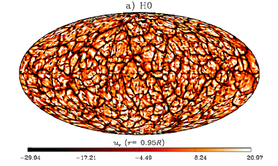
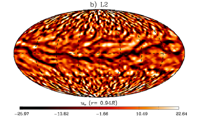
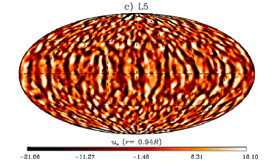
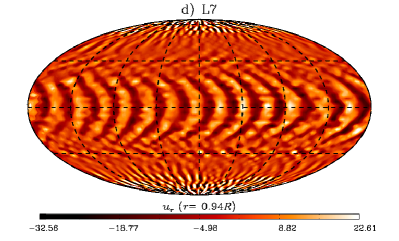
Figure 2: Mollweide projection of the vertical velocity, $u_{r}$, at the subsurface layer, $r=0.95R_{\odot}$, for models  H0 (without rotation),  L2,  L5 and  L7 (see Table 1). Yellow/dark color scale represent upward/downward motions.

The development and sustenance of large-scale flows depend on correlations between the components of the turbulent velocities, the so-called Reynolds stresses. The relative importance of these quantities defines the redistribution of angular momentum. Among these correlations, of particular importance are the vertical velocity and the rotation rate of the system since they define the formation of fast rotating zonal flows either at higher or lower latitudes. To understand this behaviour in our first set of numerical experiments we change the rotation rate while keeping the ambient state constant (i.e., the same gradient of potential temperature, Eq. 8).

Models  L1 to  L7 in Table 1 summarize the parameters and results for this set of simulations. The structure of the convective pattern for some representative cases is shown in Fig. 2b-d, where the radial component of the velocity at the top of the domain is presented using the Mollweide projection. The angular velocity, $\Omega/2\pi$, and the meridional circulation speed for some of these models are shown in the two leftmost panels of Fig. 3. We present the differential rotation in nHz, in the meridional flow panel the color scale corresponds to the latitudinal velocity in m/s, and the continuous (dashed) lines depict contours of the stream function with clockwise (anti-clockwise) circulation. In the next four panels we show the fluxes of angular momentum in the conservation equation (obtained by multiplying Eq. 3 by the level arm $\varpi=r\sin\theta$):

$$\frac{\partial({\rho}_{s}\overline{u}_{\phi})}{\partial t}=\frac{1}{\varpi}\nabla\cdot\left({\rho}_{s}\varpi[\overline{u}_{\phi}\overline{\bm{u}}_{\rm m}+\overline{u_{\phi}^{\prime}{\bm{u}}^{\prime}_{\rm m}}]\right),$$ (10)

where the over-line corresponds to the time and longitude average, $\overline{\bm{u}}_{\rm m}$ and ${\bm{u}}^{\prime}_{\rm m}$ are the mean and turbulent meridional ($r$ and $\theta$) components of the velocity, respectively. In steady state the left hand side of the equation vanishes remaining

$$\nabla\cdot\left({\rho}_{s}\varpi[\overline{u}_{\phi}\overline{\bm{u}}_{\rm m}+\overline{u_{\phi}^{\prime}{\bm{u}}^{\prime}_{\rm m}}]\right)=0.$$ (11)

The first term inside the divergence corresponds to the angular momentum flux due to meridional circulation and the second one is the flux due to small-scale correlations, the Reynolds stresses. Each of these terms has radial and latitudinal component,

$${\cal F}_{r}^{\rm MC} = \rho_{s}\varpi\overline{u}_{\phi}\overline{u}_{r},$$ (12)

$${\cal F}_{\theta}^{\rm MC} = \rho_{s}\varpi\overline{u}_{\phi}\overline{u}_{\theta},$$

$${\cal F}_{r}^{\rm RS} = \rho_{s}\varpi\overline{{u}_{\phi}^{\prime}{u}_{r}^{\prime}},$$

$${\cal F}_{\theta}^{\rm RS} = \rho_{s}\varpi\overline{{u}_{\phi}^{\prime}{u}^{\prime}_{\theta}}.$$

A more illustrative representation of these quantities is in the cylindrical coordinates $\varpi$ and $z$ thus:

$${\cal F}_{\varpi} = {\cal F}_{r}\sin\theta+{\cal F}_{\theta}\cos\theta,$$ (13)

$${\cal F}_{z} = {\cal F}_{r}\sin\theta-{\cal F}_{\theta}\cos\theta.$$

All these quantities were computed in the statistically steady state attained after a long time interval depending on the rotation rate, and averaged in time for 3.4 years.

In the case of the slower rotation rate, $\Omega_{0}=\Omega_{\odot}/4$ (run  L1), the convective pattern exhibits big convection cells which are slightly elongated in the direction opposite to the rotation. They span the range $\sim\pm 45^{\circ}$ of latitude. As for the mean flows, the azimuthal motion is slower at the equator than at the higher latitudes (left panel of Fig. 3a). The transport of angular momentum due to Reynold stress in the direction of $\varpi$ is negative at all latitudes (third panel of Fig. 3a), indicating that the rotation increases inwards. The most important contribution to the angular momentum flux is, however, the meridional circulation (rightmost panel of Fig. 3a). Single large scale meridional flow cells develops at each hemisphere. The circulation is counterclockwise (clockwise) in the northern (southern) hemisphere (second panel of Fig. 3a). This flow transports the angular momentum from the lower to higher latitudes so that the zonal flow is accelerated in the direction of rotation at latitudes between $30^{\circ}$ and $80^{\circ}$.

Increasing the rotation rate to $\Omega_{0}=\Omega_{\odot}/2$ (Run L2) or $\Omega_{0}=0.57\Omega_{\odot}$ (Run L3) we find that the convection cells are concentrated in a band around $\sim\pm 30^{\circ}$ latitude. In this region the cells are mostly elongated in the longitudinal direction (Fig. 2b). Similarly to the previous model, the latitudinal differential rotation is anti-solar (Fig. 3b). However, the radial negative shear at the equator starts not at the base of the convection zone, like in case  L1, but at $r\simeq 0.73R_{\odot}$. Between $0.7R_{\odot}<r<0.73R_{\odot}$ the plasma rotates faster than the rotating frame. In this case the largest contribution to the mixing of angular momentum comes again from the meridional circulation. However, this time two strong meridional flow cells in radius are formed in each hemisphere. In Run L2 the latitudinal velocities are so high ($\sim 40$ m/s) that the flow crosses from one hemisphere to another (second panel of Fig. 3b). Thus, the meridional flow is not fully symmetric across the equator even after a long temporal average.

In runs  L4 and  L5 the contributions of meridional circulation and Reynold stresses to the flux of angular momentum are similar. For these cases the plasma at lower latitudes rotates roughly at the same rate as the rotating frame. Above $\sim 60^{\circ}$ latitude the zonal flow decelerates and has the minimal rotation rate at the poles. The meridional flow shows a multicellular pattern with three or more cells in radius per hemisphere, with latitudinal velocities of $\sim 10$ m/s.

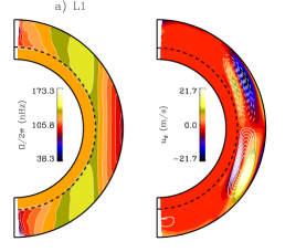
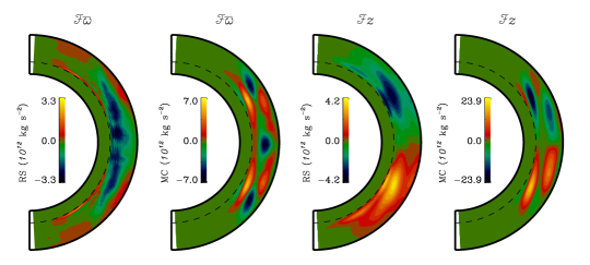
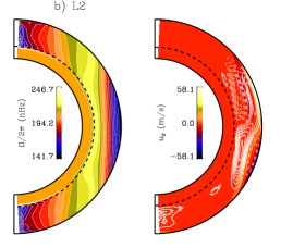
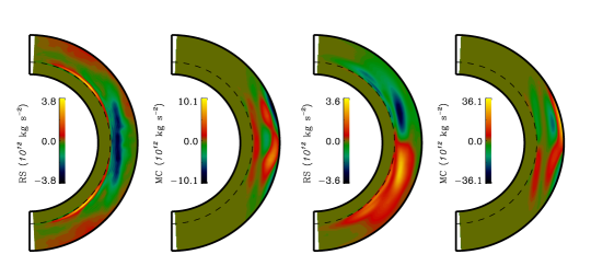
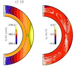
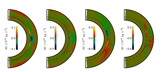
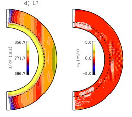
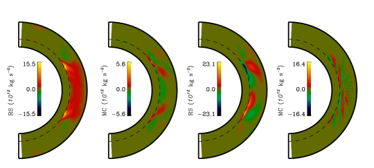
Figure 3: Differential rotation, meridional circulation (panels 1 and 2 from left to right in each row) and angular momentum flux components of Eq. (13): ${\cal F}_{\varpi}^{RS}$, ${\cal F}_{\varpi}^{MC}$, ${\cal F}_{z}^{RS}$ and ${\cal F}_{z}^{MC}$ (panels 3 to 6 from left to right), for the simulations  L1,  L2,  L6 and  L7 (top to bottom). All the profiles correspond to mean azimuthal value averaged over $\sim 3$ years during the steady state phase of the simulation.

Run  L6 ($\Omega_{0}=\Omega_{\odot}$) shows a rotation profile accelerated at the equator (Fig. 3c). Similar to the Sun, the rotation decreases monotonically towards the poles, and is in iso-rotation with the stable layer of the domain at middle latitudes. In this case the Reynolds stress components of the angular momentum flux dominate over the meridional circulation components. Although at lower latitudes, at the bottom of the convection zone ${\cal F}^{RS}_{\varpi}$ is negative, it changes sign above $r\sim 0.85R_{\odot}$. However, ${\cal F}^{RS}_{z}$, which transports the angular momentum towards the equator is more important. Something similar happens in the fastest rotating case,  L7 ($\Omega_{0}=2\Omega_{\odot}$, Fig. 3d) where the Reynolds stress drive the differential rotation. In this case, however, the transport along the rotation axis, ${\cal F}^{RS}_{\varpi}$, is the most important flux component. The rotation is faster at the equator and slower at the poles, but it exhibits jets of slow rotation in a mid latitude range which corresponds to a cylinder tangent to the base of the convection zone. The term ${\cal F}^{MC}_{z}$ has larger values but varies quickly in radius and latitude. Thus, there are no organized meridional circulation flows capable to effectively advect the angular momentum.

Figure 4: Radial profiles of the $\Theta_{e}$ for models L6, L8 and L9 as indicated in the legend.

Thus, in general, the differential rotation establishes as a competition between the buoyant and Coriolis forces. When buoyancy dominates then the differential rotation is of the anti-solar type, and when the Coriolis force rotation dominates the rotation is solar-like. To demonstrate this point we have performed the simulations labeled as  L8 and L9 in Table 1, for which the rotation has the solar value, but the profile of $\Theta_{e}$ was modified to decrease and increase the buoyancy term by making the stratification less and more superadiabatic, respectively (see Fig. 4). The model with less superadiabatic stratification,  L8, develops a faster rotating equator as a consequence of the dominant role of the Corioles force. The distribution of the angular momentum fluxes seems to be an intermediate case between the models  L6 and  L7 (Fig. 6a). On the other hand, a more superadiabatic $\Theta_{e}$ results in antisolar rotation because the buoyancy force dominates in this case. The results of this model are compatible with the case  L2 or  L3 (Fig. 6b). Another way to modify the adiabaticity of the system is considering different relaxation times, $\tau$ ($1/\alpha$ in Eq. 4). We have verified in simulations not presented here that models with shorter $\tau$ develop small fluctuations of $\Theta^{\prime}$, so that the final profile of $\Theta$ is more superadiabatic. Also, models with longer $\tau$ develop large fluctuations that tend to homogenize the potential temperature in the bulk of the convection zone, leading to a less superadiabatic system. Changes in $\tau$, however, are not as important as directly modifying the profile of $\Theta_{e}$.

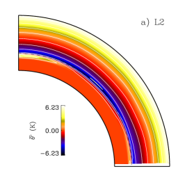
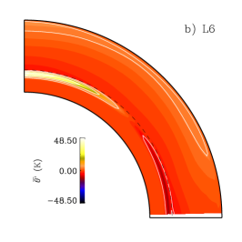
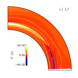
Figure 5: Azimuthal average of $\Theta^{\prime}$ for three different rotation rates corresponding to models  L2,  L6 and  L7.

It is important to notice that qualitatively the shape of the iso-rotation contours does not depend on the dominance of the buoyancy or Coriolis forces; in all cases the rotation contours are aligned along the rotation axis. To study the role of baroclinicity in the resulting Taylor-Proudman balance, in Fig. 5 we plot the azimuthal average of the potential temperature fluctuation, $\overline{\Theta^{\prime}}(r,\theta)$, for three representative models:  L2,  L6 and  L7. Slow rotation models (L1- L3) exhibit small variations of potential temperature predominantly in the radial direction. In rapid rotating models (L4- L7), below the convection zone, $\overline{\Theta^{\prime}}$ aquires larger values, it is positive at the poles and negative at the equator, indicating warmer poles. However, within the convection zone, this latitudinal gradient does not propagates and $\overline{\Theta^{\prime}}$ varies mainly radially. The lack of a latitudinal gradient in temperature explains why the contours or differential rotation remain cylindrical (see Eq. 1). The reasons and implications of this behavior will be explored in a different paper.

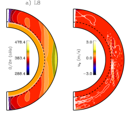
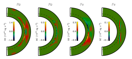
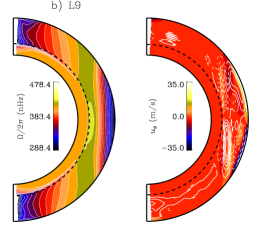
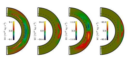
Figure 6: Same than Fig. 3 but for models a)  L5 and b)  L6. More (less) vigorous convection leads also to models with slower (faster) equator. The results are comparable to those of models  L6 or  L7 and  L2, respectively.

The transition between the solar and anti-solar rotation regimes (faster or slower equator) has been obtained since the early models of Gilman (1976) where he compared the Rayleigh with the Taylor numbers. In his Fig. 6 he depicts the regimes for transition between solid rotation, equatorial acceleration and high latitude acceleration. Similar results for the differential rotation and meridional circulation in the context of rotation of gas planets were recently reported by Gastine et al. (2013). Performing simulations for different rotation rates they found a sharp transition from the prograde to retrograde rotation of equatorial regions. They compared the Rossby number at the equator with the Rayleigh number at a mid depth, $\mbox{\rm Ra}^{*}$, and found that this transition occurs at $\mbox{\rm Ra}^{*}\sim 1$. In this paper, we compare the differential rotation parameter, defined in Eq. (9) with the Rossby number as it is depicted in Fig. 7. For the models with the same ambient state we find that the sharp transition between the prograde and retrograde regimes occurs at $\mbox{\rm Ro}\simeq 0.063$ ($\mbox{\rm Ra}^{*}\simeq 3$ in Table 1), indicated by the vertical dashed line in Fig. 7. In models with the same rotation rate but with higher (lower) superadiabaticity (models  L8 and  L9), the transition can happen at lower (higher) values of Ro. It is noteworthy to mention that the model  L6 is in a good agreement with the solar value of $\chi_{\Omega}$, indicated by the horizontal dashed-dotted line. For the model with faster rotation,  L7, the differential rotation parameter, $\chi_{\Omega}$, decreases. Here it happens due to the formation of a cylinder of slow rotation at intermediate latitudes. However, similar global simulations of fast rotating stars also show a decrease in the latitudinal differential rotation (Brown et al. 2008; Dubé & Charbonneau 2013). Käpylä et al. (2011b) also explored the transition from anti-solar to solar-like differential rotation in compressible simulation of convection in spherical wedges. In their Fig. 17 they compare the rotation parameter with the Coriolis number (inverse to Ro). Unlike our results and those in Gastine et al. (2013), in their case this transition seems to be smoother. However, due to all these differences in the model and experimental design this comparison remains inconclusive and warrants further studies.

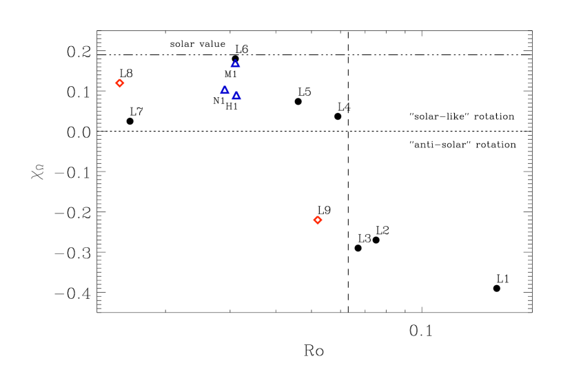
Figure 7: Differential rotation parameter, $\chi_{\Omega}$ (Eq 9), as function of the Rossby number, Ro for the simulation models defined in Table 1. The dashed vertical line at $\mbox{\rm Ro}=0.063$ indicates the sharp transition between ”solar”-type (prograde) and ”antisolar” (retrograde) regimes of the differential rotation. The dashed-dotted line indicates the solar value of $\chi_{\Omega}$.

3.2 Convergence test

As a test for the implicit SGS model, we performed a set of simulations presented for the same stratification ($\Theta_{e}$) and the same rotation rate ($\Omega_{\odot}$) but for different mesh resolutions. Run  L6, presented in the previous section was for a relatively coarse grid model with $128\times 64\times 47$ mesh points. Models M1 and L1 have $2$ and $4$ times higher resolution, respectively. Snapshots of the vertical velocity for the cases  L6,  M1 and  H1 are shown, from top to bottom panels, in Fig. 8. In all three cases convective “banana” cells elongated along the rotation axis appear in a belt of $\pm 30^{\circ}$. However, the scale of these banana cells depends on the resolution, i.e., a larger number of azimuthal modes seems to be excited for higher resolutions. The higher latitudes are populated with smaller and more symmetrical convection cells whose horizontal scale also decreases with the increasing of the resolution.

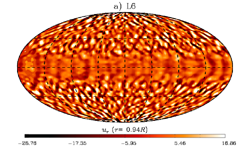
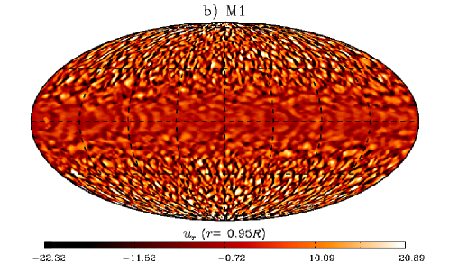
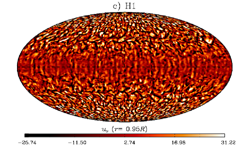
Figure 8: Snapshots of vertical velocity, $u_{r}$ for models  L6,  M1 and  H1 (Table 1) with lower, intermediate and higher grid resolution (from top to bottom).

To study the energetics of the interacting large and small scales for each of these simulations we have computed the power spectrum of the kinetic energy at a given radius, using the Fourier transform in the azimuthal direction:

$${\hat{u}}_{m}=\int{\bm{u}}(r_{t},\theta,\phi)\exp(im\phi)\frac{d\phi}{2\pi},$$ (14)

where $m$ is the azimuthal wave number, and the power spectrum definition (Mitra et al. 2009):

$$E_{u}=\langle{\hat{u}}_{m}^{2}\rangle_{\theta},$$ (15)

where the brackets denote average over latitude. Note that $\sum{E_{u}}=\langle{\bm{u}}^{2}\rangle$. The spectra for models  L6,  M1 and  H1 are plotted in Fig. 9. For the coarser resolution (continuous black line) the spectrum shows an energy decay from the smaller wavenumber up to $7\lesssim m\lesssim 15$. There are peaks of power at $m\simeq 5$ and $m\simeq 7$, which probably correspond to the scales of the banana cells. From $m\simeq 15$ to the smallest resolved scale, $m=64$, there are two different sub-ranges, one of which is compatible with the inertial turbulent decay (although not exactly following the Kolmogorov $k^{-5/3}$ law, see dot-dashed line) up to $m\simeq 30$, followed by a faster decay. In total, the energy spectra spans $\sim 3$ orders of magnitude. The spectrum for the run M1 (red line) is similar to  L6, but in this case the excess of power is at $m\simeq 6$. There is a plateau of energy from $10\lesssim m\lesssim 20$ followed by a decay up to the smallest wave number $m=128$. The model H1 with higher resolution (blue line) does not have a plateau, and the energy seems to decay continuously, with a seemingly inertial sub-range between $12\lesssim m\lesssim 30$. The peak at $m\simeq 12$ contains the energy of thin banana cells observed in this simulation. In total this model spans $\sim 5$ orders of magnitude in energy. For comparison we have plotted also the power spectrum of the models without rotation for low,  L0, and high,  H0, resolutions (black and blue dotted lines). Evidently the convective energy is higher in the models without rotation. It is interesting how this simulations show a turbulent decay consistent with $k^{-5/3}$ which spans several orders of magnitude in energy and for a long range of scales.

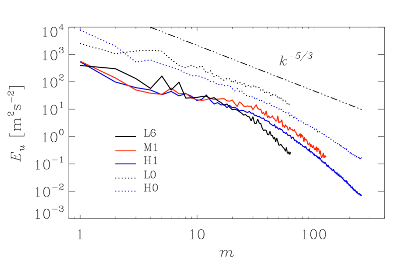
Figure 9: Power spectrum of the velocity field at $r=0.95R_{\odot}$ as a function of the azimuthal wavenumber, $m$, for simulations with different numerical resolution,  L6,  M1 and  H1 (see legend and Table 1). Continuous (dotted) lines correspond to the models with (without, models  L0 and  H0) rotation. The dot-dashed line indicates the $-5/3$ power decay.

Similarly to Fig. 3, Fig. 10 shows the profiles of differential rotation and meridional circulation obtained for models  M1 and  L1, as well as the angular momentum flux components. In model  M1 the mean rotation and meridional flows slightly resemble those of model  L6. In this case, however, the rotation shows a band of rotation with the speed of the stable layer, which spans over a large latitudinal extent. Both quantities, the Rossby number, Ro, and the rotation parameter, $\chi_{\Omega}$ are similar to those of model  L6, so that this case appears almost at the same position in Fig. 7. Regarding the angular momentum fluxes, the meridional distribution of ${\cal F}^{RS}_{\varpi}$ and ${\cal F}^{RS}_{z}$ is qualitatively similar to  L6. In the case  M1, the Reynolds stress contribution is about one half of that in case  L6 (see Fig. 10a). On the other hand, ${\cal F}^{MC}_{\varpi}$ and ${\cal F}^{MC}_{z}$ increase by a factor of two. Given the resemblance in the Reynolds stresses profiles, the differential rotation does not differ abruptly between cases  L6 and  M1. The meridional motions are, however, more pronounced in this case. Like in case  L6, there are several cells in the meridional flow profile elongated in the $z$ direction.

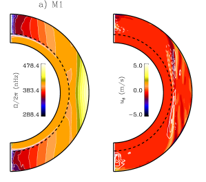
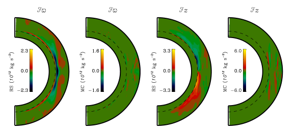
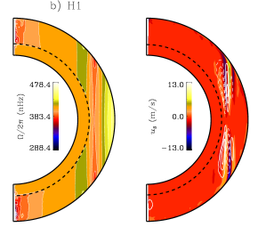
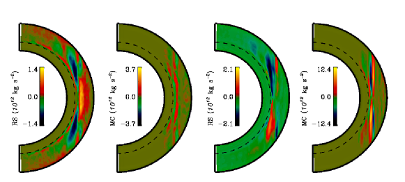
Figure 10: Same than 3 but for models  M1 and  H1 with $256\times 128\times 94$ and $512\times 256\times 188$ mesh points, respectively.

This contribution of meridional circulation to the angular momentum flux appears further enhanced in the high resolution model,  H1 (Fig. 10b). Although there is an equatorial acceleration due to a positive ${\cal F}^{RS}_{\varpi}$ flux, both ${\cal F}^{RS}_{\varpi}$ and ${\cal F}^{RS}_{z}$ are decreased in amplitude. Most importantly, there is no morphological similarity to the cases  L6 and  M1. This leads to a different profile of $\Omega$. Instead of a continuous decrease with latitude, there is a retrograde jet which appears at the surface between $~{}20^{\circ}$ and $~{}40^{\circ}$. This seems to be the consequence of meridional motions aligned along the tangent cylinder at $r\simeq 0.71R_{\odot}$. Another prograde jet appears at mid latitudes, from there up to the poles the azimuthal velocity equals the rotation rate of the frame, with a slight decrease towards the poles. In this case the meridional motions enhance ${\cal F}^{MC}_{\varpi}$ and ${\cal F}^{MC}_{z}$ by another factor of 2.

It is surprising that although the Rossby number, Ro, is similar for the models with three different resolutions, indicating that the balance between the Coriolis and buoyancy forces is roughly the same, in case  H1 the value of $\chi_{\Omega}$ ($\simeq 0.09$) is smaller than in the lower resolution models  L6 and  M1, while ${\cal F}^{MC}$ is larger. It might be the case that when a more complex and turbulent flow develops, small-scale motions contributing to the angular momentum transport diffuse on shorter timescales so that the Coriolis force does not affect them. The appearance of these new scales of motion might also change the role of the sub-grid scale transport, relegating its action to scales not resolved. The situation could be that the smallest resolved scales are already modifying the system. The question that arises, and deserves further investigation, is why these effects are not captured by the sub-grid scale transport in the coarser resolution cases? It is puzzling why our model  L6 with the rather coarse resolution reproduces the solar rotation closer than the higher resolution models,  M1 and  L1. Perhaps it may be necessary to include explicit eddy transport in the higher resolution models (i.e., include in the equation an explicit term for the turbulent heat diffusion or for the viscosity) in order to increase the efficiency of the unresolved turbulent transport. In other words, this will modify the effective Prandtl number of the simulation. Another possibility could be to readjust the parametrized turbulent heat flux profile, $\Theta_{e}$.

3.3 The solar near-surface shear layer

In the upper part of the solar convection zone the velocities are such that the turnover time is of the order of minutes (for granulation) or hours (super-granulation). These time scales are smaller when compared with the solar rotation period, $28$ days, indicating that there the buoyancy force is dominating over the Coriolis counterpart. Observations indicate that in this region the radial shear is negative, i.e., the angular velocity decreases with radius. In the simulations described in the previous sections, an inward angular momentum flux is clearly observed in the buoyant dominated regime. It corresponds to an angular velocity which decreases radially outwards. In order to simulate the buoyancy dominated regime, we can take advantage of our formulation of the energy equation and impose a rapid decrease of the potential temperature in the upper part of the convection zone. Although radiative cooling is not considered in the simulations, this sharp decline of the potential temperature (or entropy) occurs indeed at the upper part of the convection zone due to hydrogen ionization.

In the model labeled as  N1 we extend the domain in the radial direction up to $r=0.985R_{\odot}$ and modify the ambient state (Eq. 7) by considering the polytropic index

$$m(r)=m_{r} + \Delta m\frac{1}{2}\left[1+{\rm erf}\left(\frac{r-r_{tac}}{w_{t}}\right)\right]$$

$$+ \Delta m_{2}\frac{1}{2}\left[1+{\rm erf}\left(\frac{r-r_{nssl}}{w_{t}}\right)\right]\;,$$

where $\Delta m_{2}=m_{nssl}-m_{cz}$, with $m_{nssl}=1.4996$ and $r_{nssl}=0.96R_{\odot}$ (see black dotted line in Fig. 11).

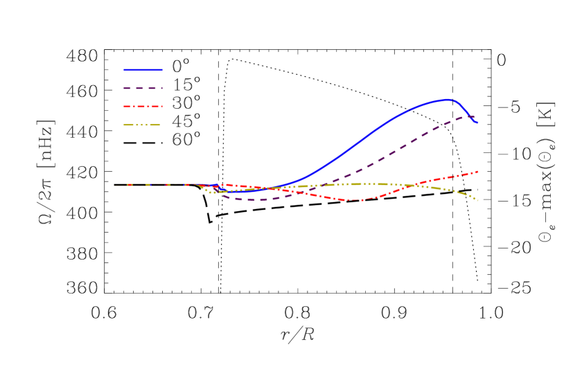
Figure 11: Radial profile of the simulated angular velocity for model  N1. Different line styles and colors correspond to different latitudes as indicated in the legend. Dotted line indicates the radial profile of the $\Theta_{e}$ (Eq. 3.3). At equatorial latitudes the angular velocity decays at the upper part of the domain (blue line).

The convection pattern, illustrated by the radial velocity field, at the top of the domain ($r=0.98R_{\odot}$, upper panel of Fig. 12) resembles the model  M1 (middle panel of Fig. 8). Elongated convective structures are observed at lower latitudes, however, these patterns are not the banana cells observed in the model  M1 but rather smaller convection cells organized along the banana cells located below the solar surface. A snapshot of the radial velocity at $r=0.94R_{\odot}$ clearly shows that the banana cells still exist below the surface (bottom panel of Fig. 12).

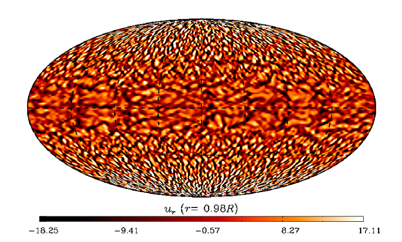
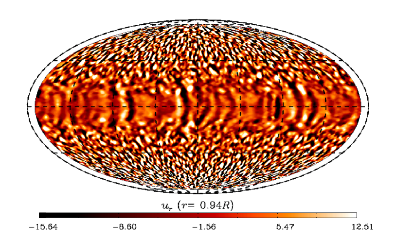
Figure 12: Snapshots of vertical velocity, $u_{r}$ (in m/s), of the model  N1. Upper and bottom panels correspond to $r=0.98R_{\odot}$ and $r=0.94R_{\odot}$.

The power spectrum at two different depths for this model shown in Fig. 13 indicates an excess of power at $m=3$ and $m=5$ for $r=0.98R_{\odot}$. There are several peaks of power between $10\lesssim m\lesssim 20$ corresponding to the smallest resolved scales. For $r=0.94R_{\odot}$ there is no peak which could be identified with the banana cells, however the peaks at large scales do not appear. The peaks of the smaller scales remain at the same values of the angular degree.

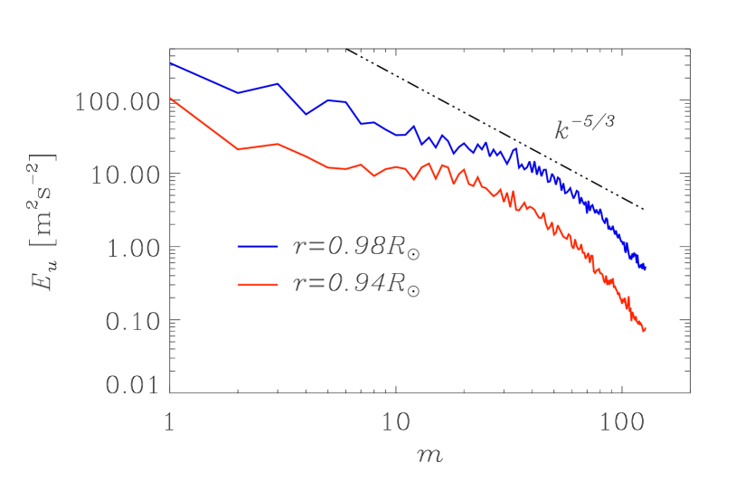
Figure 13: Power spectrum of the kinetic energy for the model  N1. The blue and red lines correspond to $r=0.98R_{\odot}$ and $r=0.94R_{\odot}$, respectively. The dotted-dashed line indicates the Kolmogorov $5/3$ turbulent decay law.

Like in the Sun, the rotation profile shows acceleration at the equator. Above $r=0.96R_{\odot}$ the rotation decreases with radius at lower latitudes (see blue line in Fig. 11). This negative shear does not remain for latitudes above $15^{\circ}$, and the contrast of differential rotation in this case is $\chi_{\Omega}=0.087$. Our interpretation is that the near-surface shear layer is associated with an inwards transfer of the angular momentum as a consequence of fast convective motions near the surface in the buoyancy dominated regime. The fact that this negative shear does not spread to high latitudes could be related to the width of the upper layer. A thicker near-surface layer could induce meridional motions transporting the angular momentum in the latitudinal direction. It might also be associated with the vertical contours of rotation obtained in our model (different from the solar rotation profile) or with the boundary conditions.

4 Discussion

Large scale flows in rotating turbulent convection, like in giant planets and stars, are developed due to collective turbulent effects. These flows are important in astrophysics since they could explain the observed patterns of surface differential rotation and, in addition, because they could be responsible for the generation of large-scale magnetic fields via the dynamo process.

In this paper we have explored the development of these large scale flows in global simulations of a convective envelope whose stratification resembles the solar interior. Although our main goal is study the pattern of differential rotation observed in the Sun, our results with different rotation rates are applicable also to solar-like stars.

The model considered here has proven to work well in simulating stellar interiors. The inviscid numerical method allows higher turbulent levels even with a coarse resolution. Besides, the energy formulation allows convection development in an slightly super-adiabatic state, which is expected to happen in an environment where the radiative flux is small.

In our numerical experiments we have obtained convective patterns, rotation and meridional circulation profiles for solar-like stars for a broad range of rotation rates. The basic properties of the flow structure are compatible with previous results of rotating convection obtained with different numerical codes (e.g., Käpylä et al. 2011b; Gastine et al. 2013). The Reynolds stress components computed from our simulations also agree with previous results in spherical geometry (e.g., Käpylä et al. 2011b) and partially agree with the mean-field theory of Lambda-effect (Rüdiger & Kitchatinov 2007).

We have explained the develpment of differential rotation as a consequence of the competition between buoyancy and Coriolis forces. This balance results in different Reynolds stress profiles which define the angular momentum distribution. For slow rotating models where buoyancy dominates, the most important contribution to the angular momentum flux comes from the meridional circulation, which results from the turbulent correlation $\langle u_{r}^{\prime}u_{\theta}^{\prime}\rangle$. For large Rossby numbers the results show either one (model  L1) or two (models  L2 and  L3) meridional cells per hemisphere.

For the rapidly rotating models the correlations $\langle u_{\phi}^{\prime}u_{\theta}^{\prime}\rangle$ and $\langle u_{\phi}^{\prime}u_{r}\rangle$ dominate, and $\langle u_{r}^{\prime}u_{\theta}^{\prime}\rangle$ might have only a marginal contribution. The differential rotation forms due to these components of the Reynolds stress and the meridional flow is formed due to inertial forces due to the rotation (Miesch & Hindman 2011). The meridional circulation exhibit several cells forming at each hemisphere. This result was found in other global convection simulations (e.g., Brun & Toomre 2002; Käpylä et al. 2011b; Ghizaru et al. 2010). However, the formation of several circulation cells is at odds with hydrodynamic mean-field models.

In order to obtain a solar-like differential rotation profile, our simulations require convective velocities of the order of m/s in the bulk of the convection zone. The Rossby number associated with this rotation rate and $u_{\rm rms}$ is of the order of $10^{-2}$ which defines the Sun as a fast rotator, see Fig. 7. Furthermore, the models close to the transition between anti-solar and solar-like differential rotation also show multiple circulation cells. Recent observational results also indicate that the Sun has more than one cell (Hathaway 2012; Zhao et al. 2012, 2013). Further studies are required, however, to clarify this issue.

We have also shown that the transition between anti-solar to solar-like rotation could also be obtained by changing the forcing of the system, i.e., making convection more or less vigorous (models  L3,  L8 and  L9). However, as mentioned before, for the solar rotation rate, only the ambient state defined in Eqs. (6 to 8) results in a fair agreement with the observed properties described in Introduction as items (i) to (iv). In the model  L6 we have been able to satisfy the properties (i) and (iii). An important result is the formation of the tachocline at the interface between stable and unstable layers.

In all the models presented here the rotation contours have cylindrical shape. Although at just below the tachocline a latitudinal gradient in $\Theta^{\prime}$ is observed in the rapid rotating simulations, it is not transported to the inner convection zone, thus being insufficient to break the columnar rotation. The solar rotation property (ii) is not reproduced for our model. A different choice of the ambient state $\Theta_{e}$ has proven to be able to create radial contours of rotation at middle an high latitudes (Racine et al. 2011). On the other hand, Warnecke et al. (2013) have obtained conical rotation profiles at lower latitudes by considering an extended domain where the solar convection zone is surrounded by a simplified coronal model. We believe that a more fundamental property (including the contribution of the magnetic field) of the plasma could be the responsible for the radial rotation profiles. A detailed study of this will be the subject of a forthcoming paper.

To tackle the formation of the near-surface shear layer, property (iv), we have constructed a model with an extended radial domain up to $r=0.985R_{\odot}$. In the outer 6% of the domain the entropy of the ambient state decreases rapidly with radius. The results of the model  N1 show that the Rossby number increases in this thin layer to values above $\mbox{\rm Ro}=0.1$. This indicates that convection is vigorous in this region, evolves on a short timescale, and is only marginally affected by rotation. In this case, above $r=0.96R_{\odot}$ the angular velocity decreases with radius at near equatorial latitudes $\lesssim 15^{\circ}$. Due to the thin width of the layer no poleward meridional circulation (like the one observed in slow rotating models) is formed due to this negative shear. Similar results have been obtained by Käpylä et al. (2011a) and Gastine & Wicht (2012) with the use of a strong density stratification. Although we keep the adiabatic background stratification constant in the energy equation, the density constrast associated with the ambient state, $\rho_{e}$, increases. Thus, both methods seem to be equivalent. In order to reproduce a near-surface shear layer spaning over all latitudes a further extended radial domain is perhaps required. Tilted contours of rotation in the bulk of the convection zone might also facilitate the formation of this layer such as it is observed.

We have tested the convergence of our models by increasing the resolution of the model L6 by a factor of $2$ and $4$ in models  M1 and  H1, respectively. The results show that for higher resolutions the solar-like differential rotation profile disappears in the deep convection zone and is reduced at the surface. We noticed that that meanwhile the Rossby number remains roughly constant, the contribution of the Reynolds stress flux decreases and the meridional circulation flux increases. This indicates that the smaller scales resolved when the turbulence of the system is increased are modifying the mixing of angular momentum in an unexpected way. This issue has been found and studied in previous works (Miesch et al. 2000; Elliott et al. 2000; Brun & Toomre 2002), by exploring different parameter regimes and boundary conditions. Brun & Toomre (2002) found that a solar-like latitudinal difference in $\Omega$ could be achieved at higher Reynolds number by decreasing the Prandtl number. This implies a more homogeneous and efficient exchange of heat and filtering certain scales. This kind of analysis involves the use of explicit dissipative terms with coefficients having eddy values (i.e., a different SGS model) and is subject for our future work.

References

- Baliunas & Vaughan (1985) Baliunas, S. L., & Vaughan, A. H. 1985, ARAA, 23, 379
- Brandenburg & Subramanian (2005) Brandenburg, A., & Subramanian, K. 2005, PhR, 417, 1
- Brown et al. (2008) Brown, B. P., Browning, M. K., Brun, A. S., Miesch, M. S., & Toomre, J. 2008, ApJ, 689, 1354
- Brown et al. (2010) —. 2010, ApJ, 711, 424
- Browning et al. (2006) Browning, M. K., Miesch, M. S., Brun, A. S., & Toomre, J. 2006, ApJ, 648, L157
- Brun et al. (2004) Brun, A. S., Miesch, M. S., & Toomre, J. 2004, ApJ, 614, 1073
- Brun & Toomre (2002) Brun, A. S., & Toomre, J. 2002, ApJ, 570, 865
- Charbonneau (2010) Charbonneau, P. 2010, Living Reviews in Solar Physics, 7, 3
- Christensen & Aubert (2006) Christensen, U. R., & Aubert, J. 2006, Geophysical Journal International, 166, 97
- Corbard & Thompson (2002) Corbard, T., & Thompson, M. J. 2002, Sol. Phys., 205, 211
- Cossette et al. (2013) Cossette, J.-F., Charbonneau, P., & Smolarkiewicz, P. K. 2013, ApJL, 777, L29
- De Rosa et al. (2002) De Rosa, M. L., Gilman, P. A., & Toomre, J. 2002, ApJ, 581, 1356
- Domaradzki et al. (2003) Domaradzki, J. A., Xiao, Z., & Smolarkiewicz, P. K. 2003, Physics of Fluids, 15, 3890
- Dubé & Charbonneau (2013) Dubé, C., & Charbonneau, P. 2013, ApJ, 775, 69
- Elliott et al. (2000) Elliott, J. R., Miesch, M. S., & Toomre, J. 2000, ApJ, 533, 546
- Elliott & Smolarkiewicz (2002) Elliott, J. R., & Smolarkiewicz, P. K. 2002, International Journal for Numerical Methods in Fluids, 39, 855
- Gastine & Wicht (2012) Gastine, T., & Wicht, J. 2012, Icarus, 219, 428
- Gastine et al. (2013) Gastine, T., Wicht, J., & Aurnou, J. M. 2013, Icarus, 225, 156
- Germano et al. (1991) Germano, M., Piomelli, U., Moin, P., & Cabot, W. H. 1991, Physics of Fluids, 3, 1760
- Ghizaru et al. (2010) Ghizaru, M., Charbonneau, P., & Smolarkiewicz, P. K. 2010, ApJL, 715, L133
- Giles et al. (1997) Giles, P. M., Duvall, T. L., Scherrer, P. H., & Bogart, R. S. 1997, Nature, 390, 52
- Gilman (1976) Gilman, P. A. 1976, in IAU Symposium, Vol. 71, Basic Mechanisms of Solar Activity, ed. V. Bumba & J. Kleczek, 207
- Gizon & Rempel (2008) Gizon, L., & Rempel, M. 2008, Sol. Phys., 251, 241
- Guerrero et al. (2013) Guerrero, G., Smolarkiewicz, P. K., Kosovichev, A., & Mansour, N. 2013, ArXiv e-prints
- Hall (2008) Hall, J. C. 2008, Living Reviews in Solar Physics, 5, 2
- Hanasoge et al. (2012) Hanasoge, S. M., Duvall, T. L., & Sreenivasan, K. R. 2012, Proceedings of the National Academy of Science, 109, 11928
- Hathaway (2012) Hathaway, D. H. 2012, ApJ, 760, 84
- Hathaway & Rightmire (2010) Hathaway, D. H., & Rightmire, L. 2010, Science, 327, 1350
- Käpylä et al. (2011a) Käpylä, P. J., Mantere, M. J., & Brandenburg, A. 2011a, Astronomische Nachrichten, 332, 883
- Käpylä et al. (2012) —. 2012, ApJL, 755, L22
- Käpylä et al. (2011b) Käpylä, P. J., Mantere, M. J., Guerrero, G., Brandenburg, A., & Chatterjee, P. 2011b, A&A, 531, A162
- Kitchatinov & Olemskoy (2012) Kitchatinov, L. L., & Olemskoy, S. V. 2012, MNRAS, 423, 3344
- Kitchatinov & Ruediger (1995) Kitchatinov, L. L., & Ruediger, G. 1995, A&A, 299, 446
- Kosovichev (1996) Kosovichev, A. G. 1996, ApJ, 469, L61
- Lipps & Hemler (1982) Lipps, F. B., & Hemler, R. S. 1982, Journal of Atmospheric Sciences, 39, 2192
- Margolin & Rider (2002) Margolin, L. G., & Rider, W. J. 2002, International Journal for Numerical Methods in Fluids, 39, 821
- Margolin et al. (2006) Margolin, L. G., Smolarkiewicz, P. K., & Wyszogradzki, A. A. 2006, Journal of Applied Mechanics, 73, 469
- Miesch et al. (2008) Miesch, M. S., Brun, A. S., De Rosa, M. L., & Toomre, J. 2008, ApJ, 673, 557
- Miesch et al. (2006) Miesch, M. S., Brun, A. S., & Toomre, J. 2006, ApJ, 641, 618
- Miesch et al. (2000) Miesch, M. S., Elliott, J. R., Toomre, J., et al. 2000, ApJ, 532, 593
- Miesch et al. (2012) Miesch, M. S., Featherstone, N. A., Rempel, M., & Trampedach, R. 2012, ApJ, 757, 128
- Miesch & Hindman (2011) Miesch, M. S., & Hindman, B. W. 2011, ApJ, 743, 79
- Mitra et al. (2009) Mitra, D., Tavakol, R., Brandenburg, A., & Moss, D. 2009, ApJ, 697, 923
- Nelson et al. (2013) Nelson, N. J., Brown, B. P., Brun, A. S., Miesch, M. S., & Toomre, J. 2013, ApJ, 762, 73
- Prusa et al. (2008) Prusa, J. M., Smolarkiewicz, P. K., & Wyszogrodzki, A. A. 2008, Comput. Fluids, 37, 1193
- Racine et al. (2011) Racine, É., Charbonneau, P., Ghizaru, M., Bouchat, A., & Smolarkiewicz, P. K. 2011, ApJ, 735, 46
- Rempel (2005) Rempel, M. 2005, ApJ, 622, 1320
- Rüdiger & Kitchatinov (2007) Rüdiger, G., & Kitchatinov, L. L. 2007, in The Solar Tachocline, ed. D. W. Hughes, R. Rosner, & N. O. Weiss, 129
- Schou et al. (1998) Schou, J., Antia, H. M., & Basu, S. e. a. 1998, ApJ, 505, 390
- Smagorinsky (1963) Smagorinsky, J. 1963, Monthly Weather Review, 91, 99
- Smolarkiewicz (2006) Smolarkiewicz, P. K. 2006, International Journal for Numerical Methods in Fluids, 50, 1123
- Smolarkiewicz & Margolin (2007) Smolarkiewicz, P. K., & Margolin, L. G. 2007 (Cambridge University Press), 413
- Smolarkiewicz et al. (2001) Smolarkiewicz, P. K., Margolin, L. G., & Wyszogrodzki, A. A. 2001, Journal of Atmospheric Sciences, 58, 349
- Spiegel & Zahn (1992) Spiegel, E. A., & Zahn, J.-P. 1992, A&A, 265, 106
- Steenbeck et al. (1966) Steenbeck, M., Krause, F., & Rädler, K.-H. 1966, Zeitschrift Naturforschung Teil A, 21, 369
- Thompson et al. (1996) Thompson, M. J., Toomre, J., Anderson, E. R., et al. 1996, Science, 272, 1300
- Ulrich (2010) Ulrich, R. K. 2010, ApJ, 725, 658
- Warnecke et al. (2013) Warnecke, J., Käpylä, P. J., Mantere, M. J., & Brandenburg, A. 2013, ArXiv e-prints
- Zhao et al. (2012) Zhao, J., Bogart, R. S., Kosovichev, A. G., & Duvall, Jr., T. L. 2012, in American Astronomical Society Meeting Abstracts, Vol. 220, American Astronomical Society Meeting Abstracts 220, 109.05
- Zhao et al. (2013) Zhao, J., Bogart, R. S., Kosovichev, A. G., Duvall, Jr., T. L., & Hartlep, T. 2013, ApJ, 774, L29
- Zhao & Kosovichev (2004) Zhao, J., & Kosovichev, A. G. 2004, ApJ, 603, 776