Scalar Representations in the Light of Electroweak Phase Transition and Cold Dark Matter Phenomenology

Abstract

The extension of the standard model’s minimal Higgs sector with an inert $SU(2)_{L}$ scalar doublet can provide light dark matter candidate and simultaneously induce a strong phase transition for explaining Baryogenesis. There is however no symmetry reasons to prevent the extension using scalars with higher $SU(2)_{L}$ representations. By making random scans over the models’ parameters, we show that in the light of electroweak physics constraints, strong first order electroweak phase transition and the possibility of having sub-TeV cold dark matter candidate the higher representations are rather disfavored compared to the inert doublet. This is done by computing generic perturbativity behavior and impact on electroweak phase transitions of higher representations in comparison with the inert doublet model. Explicit phase transition and cold dark matter phenomenology within the context of the inert triplet and quartet representations are used for detailed illustrations.

1 Introduction

The discovery of an about 126 GeV Higgs boson  [1, 2] is yet another important support for and completion of the Standard Model (SM). The SM with minimal Higgs sector contains one complex Higgs doublet which after electroweak symmetry breaking gives a neutral CP-even Higgs boson. But one can consider a scenario with singlets, with more than one doublet or with an $N$ copies of $SU(2)_{L}$ n-tuplets where the (non standard) Higgs sector can be used to explicitly account for Baryogenesis and cold dark matter. Using these phenomena and related experimental data we set to qualitatively explore for the preferred scalar representation in the SM.

Extensive astrophysical and cosmological observations have already put dark matter (DM) as a constituent of the universe beyond any doubt. Although we still have to determine which is the candidate for the dark matter from particle physics point of view, the most popular one is considered to be the stable weakly interacting particle (WIMP) [3] for which the observed DM relic density is obtained if it’s mass lies near the electroweak scale. Apart from DM identification, one other unresolved question within SM is the observed matter-antimatter asymmetry of the universe. Such asymmetry is described by Baryogenesis scenario first put forward by Sakharov [4] and one essential ingredient of this mechanism is ’out of equilibrium process’.

Now that the study of beyond standard model (BSM) physics is being explored with the LHC, a well motivated scenario within the testable reach of LHC is Electroweak Baryogenesis [5] where out of equilibrium condition is given by strong first order phase transition. The SM has all the tools required by the Sakharov’s condition for Baryogenesis, i.e. baryon number violation at high temperature through sphalerons [6, 7, 8], C and CP violation with CKM phase and strong first order phase transition [9, 10]. However, it was shown that to avoid baryon washout by sphalerons, Higgs mass has to be below $45$ GeV for strong electroweak phase transition (EWPhT) [11, 12, 13, 14], which was later confirmed by lattice studies [15, 16, 17] and eventually it was ruled out by the LEP data [18]. Now with Higgs at $126$ GeV, clearly one can see the requirement of extending SM by new particles, possibly lying nearly the electroweak scale, which could not only provide strong EWPhT for explaining matter asymmetry but also the DM content of the universe.

One promising way is to extend the scalar sector of the SM. Within the literature there are numerous considerations for non minimal Higgs sector with various representations of the additional Higgs multiplet in order to account for Baryogenesis and/or dark matter. For instance, in the inert doublet case considered in [19, 20, 21], it was shown that it can enable one to achieve strong EWPhT with DM mass lying between $45$ GeV and $80$ GeV and predicts a lower bound on the direct detection that is consistent with XENON direct detection limit [118] (in case of sub-dominant DM, see [22]). Inert doublet is a well motivated and minimal extension of scalar sector which was first proposed as dark matter [23], was studied as a model for radiative neutrino mass generation [24], improved naturalness [25] and follows naturally [27, 26] in case of mirror families [28, 29, 30, 31] that was to fulfill Lee and Yang’s dream to restore parity [32]. The DM phenomenology regarding Inert doublet model has been studied extensively in Refs. [33, 34, 35, 36, 37, 38, 39, 40, 41, 42, 43, 44, 45, 46, 47]. Moreover, tentative $130$ GeV gamma line from galactic center can be accommodated in inert doublet framework [49]. Therefore, one can extend scalar sector by introducing higher inert representation and explore the nature of phase transition, consistency of the theory at high scale and dark matter phenomenology. In this paper, we have tried to carry out such analysis.

Apart from the doublet, one other possibility is the scalar singlet [50, 51, 52, 53, 54] (and references there) which can be accounted for strong EWPhT and light DM candidate but not simultaneously (for exceptions, see [55, 56, 57]). In case of larger representations, a systematic study for DM candidate has been performed in [61] from doublet to 7-plet of $SU(2)_{L}$ with both fermionic and scalar DM where only allowed interactions of DM are gauge interactions. Additionally, scalar multiplet allows renormalizable quartic couplings with Higgs doublet. In [62], study of DM phenomenology for such scalar multiplet was carried out for large odd dimensional and real representation and the mass of the DM turned out to be larger than the scale relevant for strong EWPhT. Besides, fermions with large yukawa couplings to Higgs can trigger strong EWPhT by producing large entropy when they decouple and also they can be viable dark matter candidates [63] but it requires some fine tuning of Higgs potential. Another approach with vector-like fermions is explored in [64].

Here we want to compare the various models extending the Higgs sector using different representations in order to find the favored representation. From the scalar sector extension, we want viable DM candidates which will trigger strong 1st order EWPhT accounting for Baryogenesis.

The paper is organized as follows. In Sec.(2) we present the potential, zero temperature mass spectrum, constraints on the size of the scalar multiplets from perturbativity and electroweak precision bounds. In Sec.(3) we present the finite temperature effective potential and studied the nature of phase transition for large multiplets. In Sec.(4) we present the relic density analysis and direct detection limit for light DM in larger multiplets. Conclusions are drawn in Sec.(5). In the appendices we present the relevant formulas.

2 Scalar Representations Beyond the Standard Model

2.1 Scalar Multiplets with Cold Dark Matter Candidates

Any scalar multiplet charged under $SU(2)_{L}\times U(1)_{Y}$ gauge group is characterized by $(J,Y)$. The electric charge for components of the multiplet is given by, $Q=T_{3}+\frac{Y}{2}$. For half integer representation $J=n/2$, $T_{3}$ ranges from $-\frac{n}{2}$ to $\frac{n}{2}$. So the hypercharge of the multiplet needs to be, $Y=\pm 2T_{3}$ for one of the components to have neutral charge and can be considered as DM. For integer representation $n$, similar condition holds for hypercharge.

When one considers the lightest component of the scalar multiplet as a good dark matter candidate [65], it’s life time has to be longer than about $10^{26}$ sec which is set by current experimental limits on fluxes of cosmic positrons, antiprotons and $\gamma$ radiation [66, 67]. Such limits on the lifetime of the DM requires new couplings to be extremely small. Therefore, it’s natural to adopt a $Z_{2}$ symmetry under which all SM particles are $Z_{2}$ even and extra scalars are $Z_{2}$ odd such a way that the new couplings don’t arise in the Lagrangian which will lead to the decay of dark matter. Also this $Z_{2}$ symmetry becomes accidental for representations $J\geq 2$ if we only allow renormalizable terms in the Lagrangian. Moreover, our study is performed in a region of parameter space where inert scalar multiplets do not develop any vev both in zero and finite temperature.

Denoting scalar multiplet as $Q$, and the SM Higgs as $\Phi$, the most general Higgs-scalar multiplet potential , symmetric under $Z_{2}$, can be written in the following form,

$$V_{0}(\Phi,Q) = -\mu^{2}\Phi^{\dagger}\Phi+M_{Q}^{2}Q^{\dagger}Q+\lambda_{1}(\Phi^{\dagger}\Phi)^{2}+\lambda_{2}(Q^{\dagger}Q)^{2}+\lambda_{3}|Q^{\dagger}T^{a}Q|^{2}$$ (2.1)

$$+ \alpha\Phi^{\dagger}\Phi Q^{\dagger}Q+\beta\Phi^{\dagger}\tau^{a}\Phi Q^{\dagger}T^{a}Q+\gamma[(\Phi^{T}\epsilon\tau^{a}\Phi)(Q^{T}CT^{a}Q)^{\dagger}+h.c]$$

Here, $\tau^{a}$ and $T^{a}$ are the $SU(2)$ generators in fundamental and Q’s representation respectively. $C$ is an antisymmetric matrix analogous to charge conjugation matrix defined as,

$$CT^{a}C^{-1}=-T^{aT}$$ (2.2)

$C$, being antisymmetric matrix, can only be defined for even dimensional space, i.e only for half integer representation. If the isospin of the reps. is $j$ then $C$ is $(2j+1)\times(2j+1)$ dimensional matrix (an explicit form of generators and $C$ matrix for the quartet are given in appendix (6.1)). The generators are normalized in such a way, so that they satisfy, for fundamental representation, $Tr[\tau^{a}\tau^{b}]=\frac{1}{2}\delta^{ab}$ and for other representations, $Tr(T^{a}T^{b})=D_{2}(Q)\delta^{ab}$. Also $T^{a}T^{a}=C_{2}(Q)$. Here, $D_{2}(Q)$ and $C_{2}(Q)$ are Dynkin index and second Casimir invariant for $Q$’s representation. The explicit form of generators, $\epsilon$ and $C$ matrix are given in the appendix. Notice that, $\gamma$ term is only allowed for representation with $(J,Y)=(\frac{n}{2},1)$.

For the doublet, real triplet, complex triplet, and the quartet the scalar multiplet $Q$ is respectively

$$\begin{pmatrix}C^{+}\\ D^{0}\equiv\frac{1}{\sqrt{2}}(S+iA)\\ \end{pmatrix}\,,\begin{pmatrix}\Delta^{+}\\ \Delta^{0}\\ \Delta^{-}\end{pmatrix}_{(Y=0)}\,,\begin{pmatrix}\Delta^{++}\\ \Delta^{+}\\ \Delta^{0}\equiv\frac{1}{\sqrt{2}}(S+iA)\end{pmatrix}_{(Y=2)}\,,\textrm{ and }\begin{pmatrix}Q^{++}\\ Q^{+}\\ Q^{0}\equiv\frac{1}{\sqrt{2}}(S+iA)\\ Q^{{}^{\prime}-}\end{pmatrix}.$$ (2.3)

In general, for the half-integer representation with $(J,Y)=(\frac{n}{2},1)$ and the Integer representation with $(J,Y)=(n,Y=0\textrm{ or }\pm 2T_{3})$, the scalar multiplets with component fields denoted as $\Delta^{(Q)}$, where $Q$ is the electric charge, are respectively

$$\bf{Q_{\frac{n}{2}}}=\begin{pmatrix}\Delta^{(\frac{n+1}{2})}\\ ...\\ \Delta^{(0)}\equiv\frac{1}{\sqrt{2}}(S+i\,A)\\ ...\\ \Delta^{(-\frac{n-1}{2})}\\ \end{pmatrix}\,\textrm{ and }\,\bf{Q_{n}}=\begin{pmatrix}\Delta^{(n)}\\ ...\\ \Delta^{(0)}\\ ...\\ \Delta^{(-n)}\\ \end{pmatrix}_{Y=0}.$$ (2.4)

For the former representation every component represents a unique field while for the latter there is a redundancy $\Delta^{(-n)}=(\Delta^{(n)})^{*}$ except the $Y\neq 0$ case for which the component are also unique.

2.2 Inert Triplet and Quartet Mass spectra

Mass spectra: Half Integer Representation with $Y=1$

We now sketch the general form of mass spectrum for the multiplet. As $Y=1$, $T_{3}$ value of the neutral component of the multiplet has to be $T_{3}=-\frac{1}{2}$. Now for Higgs vacuum expectation value, $\langle\Phi\rangle=(0,\frac{v}{\sqrt{2}})^{T}$, the term $\langle\Phi^{\dagger}\rangle\tau^{3}\langle\Phi\rangle$ gives $-\frac{v^{2}}{4}$. So masses for the neutral components, $S$ and $A$ are respectively

$$m_{S}^{2}=M_{Q}^{2}+\frac{1}{2}(\alpha+\frac{1}{4}\beta+p(-1)^{p+1}\gamma)v^{2}\,\textrm{ and }m_{A}^{2}=M_{Q}^{2}+\frac{1}{2}(\alpha+\frac{1}{4}\beta-p(-1)^{p+1}\gamma)v^{2}.$$ (2.5)

Here, $p=\frac{1}{2}\text{Dim}(\frac{n}{2})=1,2,...$ comes from $2p\times 2p$ $C$ matrix. For the charged component, with $T_{3}=j$, we have,

$$m_{(j)}^{2}=M_{Q}^{2}+\frac{1}{2}(\alpha-\frac{1}{2}j\beta)v^{2}.$$ (2.6)

Now because of the $\gamma$ term, there will be mixing between components carrying same amount of charge. So to write down the mixing matrix, we have considered the ordering as follows. A component of the multiplet is denoted as $|J,T_{3}\rangle$. Components below the neutral component $|\frac{n}{2},-\frac{1}{2}\rangle$ are denoted with $|\frac{n}{2},-\frac{1}{2}-m\rangle$ where, $m=1,2,....,\frac{n-1}{2}$ and corresponding charge is $Q=-m$. The piece $\langle\Phi\rangle^{T}\epsilon\tau^{a}\langle\Phi\rangle$ gives $\frac{v^{2}}{2\sqrt{2}}$. Therefore, the mixing term between between components with charge $|Q|=m$ is, $(-1)^{m+1}\frac{\gamma v^{2}}{4}\sqrt{(n+2m+1)(n-2m+1)}$. In the ordering, $(\Delta_{(\frac{1}{2})}^{+},\Delta_{(-\frac{3}{2})}^{+})$, with $m=1$, the mass matrix becomes,

$$M^{2}_{+}=\begin{pmatrix}m^{2}_{(\frac{1}{2})}&\,\,\frac{\gamma v^{2}}{4}\sqrt{(n+3)(n-1)}\\ \\ \frac{\gamma v^{2}}{4}\sqrt{(n+3)(n-1)}&\,\,m^{2}_{(-\frac{3}{2})}\end{pmatrix}$$ (2.7)

And with $m=2$ and $(\Delta_{(\frac{3}{2})}^{++},\Delta_{(-\frac{5}{2})}^{++})$ we have,

$$M^{2}_{++}=\begin{pmatrix}m^{2}_{(\frac{3}{2})}&\,\,-\frac{\gamma v^{2}}{4}\sqrt{(n+5)(n-3)}\\ \\ -\frac{\gamma v^{2}}{4}\sqrt{(n+5)(n-3)}&\,\,m^{2}_{(-\frac{5}{2})}\end{pmatrix}$$ (2.8)

and so on, for charges with $m=3,4,\ldots$.

For example, if we consider $S$ of inert doublet to be the DM candidate, then following our parameterization Eq.(2.1) and Eq.(2.3), the mass spectrum, where the mass hierarchy becomes apparent, is in the following

$$m^{2}_{S} = M^{2}_{Q}+\frac{1}{2}(\alpha+\frac{1}{4}\beta+\gamma)v^{2}$$

$$m^{2}_{A} = m^{2}_{S}-\gamma v^{2}$$

$$m^{2}_{C} = m^{2}_{S}-\frac{1}{2}(\gamma+\frac{1}{2}\beta)v^{2}$$ (2.9)

Quartet Model The immediate generalization of doublet case is the $J=3/2$ quartet case. Therefore we have carefully investigated its relic density, direct detection, it’s connection to strong EWPhT in low mass regime of DM. Apart from splitting between $S$ and $A$, $\gamma$ term also mixes two single charged components of the quartet. According to Eq.(2.7), the mass matrix for single charged fields in $(Q^{+},Q^{{}^{\prime}+})$ basis is

$$M^{2}_{+}=\begin{pmatrix}M_{Q}^{2}+\frac{1}{2}(\alpha-\frac{1}{4}\beta)v^{2}&\frac{\sqrt{3}}{2}\gamma v^{2}\\ \frac{\sqrt{3}}{2}\gamma v^{2}&M_{Q}^{2}+\frac{1}{2}(\alpha+\frac{3}{4}\beta)v^{2}\end{pmatrix}$$ (2.10)

Diagonalizing the mass matrix, we have mass eigenstates for single charged fields, $Q_{1}^{+}=Q^{+}\cos\theta+Q^{{}^{\prime}+}\sin\theta$, $Q_{2}^{+}=-Q^{+}\sin\theta+Q^{{}^{\prime}+}\cos\theta$ with $\tan 2\theta=-\frac{2\sqrt{3}\gamma}{\beta}$.

Again we consider $S$ to be the dark matter. So masses of the components of the multiplet are as follows,

$$m^{2}_{S} = M^{2}_{Q}+\frac{1}{2}(\alpha+\frac{1}{4}\beta-2\gamma)v^{2}$$

$$m^{2}_{A} = m^{2}_{S}+2\gamma v^{2}$$

$$m^{2}_{Q^{++}} = m^{2}_{S}-\frac{1}{2}(\beta-2\gamma)v^{2}$$

$$m^{2}_{Q^{+}_{1}(Q^{+}_{2})} = m^{2}_{S}+(\gamma\mp\frac{1}{4}\sqrt{\beta^{2}+12\gamma^{2}})v^{2}$$ (2.11)

Because of the mixing between two single charged states, the mass relation is

$$m_{S}^{2}+m_{A}^{2}=m_{Q_{1}^{+}}^{2}+m_{Q_{2}^{+}}^{2}$$ (2.12)

The full stability analysis for the quartet potential is an involved task but for time being, we can give a partial set of necessary stability conditions by taking Higgs-scalar two dimensional complex surface $(h,\xi^{i},0,0,...)$ in field space..

$$\lambda_{1}>0\, \lambda_{2},\lambda_{3}>0$$ ,

$$\alpha+\frac{1}{4}\beta-2\gamma > -2\sqrt{\lambda_{1}(\lambda_{2}+\frac{1}{4}\lambda_{3})}\,\,\,\text{in $(h,S,0,..)$ surface}$$

$$\alpha+\frac{1}{4}\beta+2\gamma > -2\sqrt{\lambda_{1}(\lambda_{2}+\frac{1}{4}\lambda_{3})}\,\,\,\text{in $(h,A,0,..)$ surface}$$

$$\alpha-\frac{3}{4}\beta > -2\sqrt{\lambda_{1}(\lambda_{2}+\frac{3}{4}\lambda_{3})}\,\,\,\text{in $(h,Q^{++},0,..)$ surface}$$

$$\alpha-\frac{1}{4}\beta > -2\sqrt{\lambda_{1}(\lambda_{2}+\frac{1}{4}\lambda_{3})}\,\,\,\text{in $(h,Q^{+},0,..)$ surface}$$

$$\alpha+\frac{3}{4}\beta > -2\sqrt{\lambda_{1}(\lambda_{2}+\frac{9}{4}\lambda_{3})}\,\,\,\text{in $(h,Q^{\prime-},0,..)$ surface}$$ (2.13)

The last two conditions, when expressed in terms of mass eigenstates ${Q^{+}_{1},Q^{+}_{2}}$ becomes

$$\alpha\mp\frac{1}{4}\beta(1\mp 2\cos{2\theta})\pm\sqrt{3}\gamma\sin{2\theta}>-\sqrt{\lambda_{1}\lambda_{2}+\frac{1}{4}\lambda_{1}\lambda_{3}(3\mp 4\cos{2\theta}+2\cos{4\theta})}$$ (2.14)

in $(h,Q_{1,2}^{+})$ surface.

Mass spectra: Integer Representation with $Y=0$ and $Y\neq 0$ For integer representation, $\gamma$ term is not allowed. Therefore, there will not be any mass splitting between real and imaginary part of the neutral component. Moreover, for $Y=0$ or real representation, the term $Q^{\dagger}T^{3}Q$ is zero. So tree level mass spectrum is degenerate and is given by,

$$m^{2}_{\Delta}=M^{2}_{Q}+\frac{1}{2}\alpha v^{2}.$$ (2.15)

On the other hand, if $Y\neq 0$, there will be mass splitting due to $\beta$ term. Also one can choose $Y$ as, from $-n$ to $n$, to set one component to be neutral. If $T_{3}=j$, the mass is given by,

$$m^{2}_{(j)}=M^{2}_{Q}+\frac{1}{2}(\alpha-\frac{1}{2}\beta j)v^{2}$$ (2.16)

Triplet Model

A well motivated representative of this class is the Triplet with $Y=2$ because of it’s role in explaining the smallness of neutrino mass in Type-II seesaw mechanism [69]. In this case, $\Delta$ is odd under $Z_{2}$ symmetry, therefore the neutral component will not acquire any vacuum expectation value. For real triplet, the term, $\Delta^{\dagger}T_{T}^{3}\Delta$ is zero, so the mass spectrum will be degenerate and given as,

$$m^{2}_{\Delta^{+}}=m^{2}_{\Delta^{0}}=M_{\Delta}^{2}+\frac{1}{2}\alpha v^{2}.$$ (2.17)

On the other hand, for complex case, the mass spectrum is,

$$m_{S}^{2}=m_{A}^{2} = M_{\Delta}^{2}+\frac{1}{2}(\alpha+\frac{1}{2}\beta)v^{2}$$ (2.18)

$$m_{\Delta^{+}}^{2} = M_{\Delta}^{2}+\frac{1}{2}\alpha v^{2}$$ (2.19)

$$m_{\Delta^{++}}^{2} = M_{\Delta}^{2}+\frac{1}{2}(\alpha-\frac{1}{2}\beta)v^{2}$$ (2.20)

There is a relation between masses:

$$m_{\Delta^{++}}^{2}-m_{\Delta^{+}}^{2}=m_{\Delta^{+}}^{2}-m_{\Delta^{0}}^{2}=\frac{1}{4}\beta v^{2}$$ (2.21)

And the stability conditions are,

$$\lambda_{1}>0\, \lambda_{2},\lambda_{3}>0$$ ,

$$2\alpha+\beta > -2\sqrt{\lambda_{1}(\lambda_{2}+\lambda_{3})}\,\,\,\text{in $(h,\Delta^{0},0,..)$ surface}$$

$$\alpha > -2\sqrt{\lambda_{1}\lambda_{2}}\,\,\,\text{in $(h,\Delta^{+},0,..)$ surface}$$ (2.22)

$$2\alpha-\beta > -2\sqrt{\lambda_{1}(\lambda_{2}+\lambda_{3})}\,\,\,\text{in $(h,\Delta^{++},0,..)$ surface}$$ (2.23)

Because of the absence of $\gamma$ term as in half integer representation, there is no mass splitting between $S$ and $A$ of the neutral component $\Delta^{0}$. $S$ and $A$ have vector interaction with $Z$ boson that produces spin-independent elastic cross section which is already $8-9$ orders of magnitude above the CDMS direct detection bound [70] and for this reason, complex triplet or any larger integer multiplet with non zero hypercharge is not going to satisfy direct detection bound as one will require a non-zero splitting between $S$ and $A$ larger than the kinetic energy of DM in our galactic halo to make $Z-S-A$ process kinematically forbidden. Therefore, only neutral component of the real triplet can be a plausible DM candidate. In fact real triplet DM has already been studied in [62, 61, 71, 72]. In [61, 71] it was shown that observed relic density can be accounted for DM if the mass of DM lies about $2.5$ TeV. Being degenerate, one can easily see that, such particle would decouple from electroweak plasma and had no significant effect on EWPhT. But the question of having a strong first order EWPhT in complex triplet is relevant for cosmic evolution of the universe. Therefore we only focused on EWPhT in complex triplet case in a later section.

2.3 Perturbativity and EW Physics Constraints on the Size of Multiplets

Perturbativity and Renormalization Group Equations

What is the largest possible inert multiplet allowed to be added to the standard model? One possible bound comes from the beta function of $SU(2)$ gauge coupling in presence of large scalar multiplets because the addition of such large multiplet not only halts the asymptotic freedom of non-Abelian gauge couplings but also lowers the scale of landau pole with its size.

The one-loop beta function of $SU(2)$ gauge coupling for Standard Model solely augmented by a scalar multiplet of isospin $J$ is $\beta(g)=\frac{g^{3}}{16\pi^{2}}(-\frac{19}{6}+\frac{1}{9}J(J+1)(2J+1))$. It can be seen that, $\beta(g)$ remains negative only for $J\leq\frac{3}{2}$. For, $J\geq 2$, it becomes positive and hits the landau pole as shown in Fig.(1).

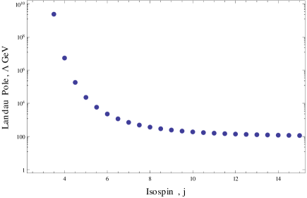
Figure 1: Landau pole with different scalar multiplet.

For instance adding a scalar multiplet with isospin $J\geq 5$ will bring the Landau pole of $SU(2)$ gauge coupling at $\Lambda\leq 10$ TeV and for $J\geq 10$, its even smaller, $\Lambda\leq 180$ GeV. Therefore, perturbativity of gauge coupling at the TeV scale sets a upper bound on the size of the multiplet to be $J\leq 5$.

Another bound on the size of the multiplet, charged under SM gauge group, is set by perturbative unitarity of tree-level scattering amplitude. In [73, 74], the $2\rightarrow 2$ scattering amplitudes for scalar pair annihilations into electroweak gauge bosons have been computed and by requiring zeroth partial wave amplitude satisfying the unitarity bound, it was shown that maximum allowed complex $SU(2)_{L}$ multiplet would have isospin $J\leq 7/2$ and real multiplet would have $J\leq 4$.

In addition, a check with 1-loop beta functions, given in appendix.(6.3), for the triplet [75] compared to the doublet [25] shows in Fig. (2) that on increasing the size of the multiplet, the scalar couplings will run faster compared to the smaller representation and will become non-perturbative much faster if one starts with large scalar coupling at EW scale.

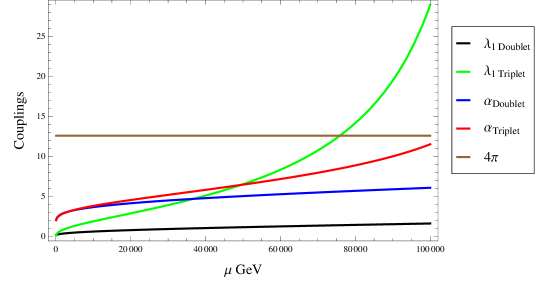
Figure 2: The running of Higgs quartic coupling $\lambda_{1}$ and coupling $\alpha$. The initial values of the couplings at energy $\mu=100$ GeV are $(\lambda_{1},\lambda_{2},\lambda_{3},\alpha,\beta,\gamma)=(0.13,0.1,0.1,2,0.1,0.1)$ for both cases. Here we can see that large values of $\alpha$ which also drives strong EWPhT, as we will see later, drives Higgs coupling to run much faster in triplet than the doublet case.

Electroweak Precision Observable

A straightforward way to observe the indirect effect of new physics is in the modification of vacuum polarization graph of $W^{\pm}$ and $Z^{0}$ boson and one convenient way to parameterize these ’Oblique correction’ is through $S$, $T$ and $U$ parameters [76, 77] (analysis of one-loop correction in SM was first done in [78]); plus V, W and X parameters [79] if new physics is at scale comparable to the EW scale. Oblique corrections are dominant over other ’non-oblique’ corrections (vertex diagram and box diagram with SM fermions as external states) because all the particles charged under SM group will couple to gauge bosons but usually only one or two particles in a theory will couple to specific fermion species.

In the present case we have only considered the quartet and because of absence of coupling between quartet fields and SM fermions, the only dominant effects will come from oblique corrections. $T$ parameter, measuring the shift of $\rho=\frac{M_{W}}{M_{Z}\cos\theta_{w}}$ from SM value due to the radiative correction by new particles, is

$$\alpha T=\frac{\Pi_{WW}(0)}{M^{2}_{W}}-\frac{\Pi_{ZZ}(0)}{M^{2}_{Z}}$$ (2.24)

where, $\Pi_{WW}(0)$ and $\Pi_{ZZ}(0)$ vacuum polarization graph of $W$ and $Z$ bosons evaluated at external momentum, $p^{2}=0$.

And quartet contribution to T parameter,

$$\frac{16\pi^{2}\alpha}{g^{2}}T = \frac{1}{M^{2}_{W}}(\frac{3}{2}\cos^{2}\theta\,F(m_{Q^{++}},m_{Q_{1}^{+}})+\frac{3}{2}\sin^{2}\theta\,F(m_{Q^{++}},m_{Q_{2}^{+}})$$ (2.25)

$$+ \frac{1}{4}(\sqrt{3}\sin\theta+2\cos\theta)^{2}\,F(m_{Q_{1}^{+}},m_{S})+\frac{1}{4}(\sqrt{3}\sin\theta-2\cos\theta)^{2}\,F(m_{Q_{1}^{+}},m_{A})$$

$$+ \frac{1}{4}(\sqrt{3}\cos\theta-2\sin\theta)^{2}\,F(m_{Q_{2}^{+}},m_{S})+\frac{1}{4}(\sqrt{3}\cos\theta+2\sin\theta)^{2}\,F(m_{Q_{2}^{+}},m_{A}))$$

$$- \frac{1}{4c^{2}_{w}M^{2}_{Z}}(F(m_{S},m_{A})+\sin^{2}2\theta\,F(m_{Q_{1}^{+}},m_{Q_{2}^{+}})$$

here,

$$F(m_{1},m_{2})=\frac{m^{2}_{1}+m^{2}_{2}}{2}-\frac{m_{1}^{2}m_{2}^{2}}{m_{1}^{2}-m_{2}^{2}}\ln\frac{m_{1}^{2}}{m_{2}^{2}}$$ (2.26)

In addition, S parameter for quartet multiplet is,

$$S = \frac{s_{w}^{2}}{8\pi}\int_{0}^{1}dx\,x(x-1)[\ln\frac{m^{2}_{Q_{1}^{+}}m^{2}_{Q_{2}^{+}}}{m^{4}_{Q^{++}}}+2\cos 2\theta\ln\frac{m^{2}_{Q_{2}^{+}}}{m^{2}_{Q_{1}^{+}}}$$ (2.27)

$$+ \ln\frac{(1-x)m^{2}_{S}+xm^{2}_{A}}{m^{2}_{Q^{++}}}+\sin^{2}2\theta\ln\frac{[(1-x)m^{2}_{Q_{1}^{+}}+xm^{2}_{Q_{2}^{+}}]^{2}}{m^{2}_{Q_{1}^{+}}m^{2}_{Q_{2}^{+}}}]$$

The best fit values of S and T parameter with ($U=0$) is [81]

$$S=0.04\pm 0.09\,\,\,\text{and}\,\,\,T=0.07\pm 0.08$$ (2.28)

Therefore, one can put constraints on S and T parameter by comparing the theoretical predictions with well measured experimental values of observables.

3 Electroweak Phase Transition (EWPhT)

3.1 Finite Temperature Effective Potential

To study the impact of large scalar multiplets on the electroweak phase transition, we have used the standard techniques of finite temperature field theory [82, 83, 84, 85, 86] (for a quick review, also see [87]). If there are multiple classical background fields $\phi_{i}$ , which act as order parameters of the thermodynamic system, the total one-loop effective potential at finite temperature is,

$$V_{eff}(\phi_{i},T)=V_{0}(\phi_{i})+V_{CW}(\phi_{i})+V_{T}(\phi_{i},T)$$ (3.1)

Here, $V_{0}$, $V_{CW}$ and $V_{T}$ are tree-level, 1-loop Coleman-Weinberg and finite temperature potential respectively. The daisy resummed [90, 89] finite temperature potential is,

$$V_{T}=\sum_{B(F)}(\pm)g_{B(F)}\frac{T^{4}}{2\pi^{2}}\int_{0}^{\infty}dxx^{2}\ln(1\mp e^{-\sqrt{x^{2}+m_{B(F)}^{2}(\phi_{i},T)/T^{2}}})$$ (3.2)

Here, $g_{B}$ and $g_{F}$ are bosonic and fermionic degrees of freedom and $\pm$ correspond to boson and fermion respectively. Thermal mass correction determined with respect to background fields $\phi_{j}$ is,

$$m^{2}_{i}(\phi_{j})\rightarrow m^{2}_{i}(\phi_{j},T)=m^{2}_{i}(\phi_{j})+\Pi_{i}(T)$$ (3.3)

where $\Pi_{i}(T)$ is the thermal self energy correction (Debye correction) and at the high temperature limit, it is of the form $T^{2}$ times coupling constants. $\Pi_{i}(T)$ measures how much particles are screened by thermal plasma from the classical background field $\phi$ (just like the Debye screening) and large screening reduces the strength of phase transition. In other words, it is the amplitude for the external particle (sourced by classical field) to forward scatter off from a real physical particle present in the thermal bath [88].

For numerical convenience, in subsequent studies, we have used the following form of the effective potential in high temperature approximation Appendix (6.2),

$$V_{eff} = V_{0}+V_{CW}+\sum_{B}g_{B}[\frac{m^{2}_{B}(\phi,T)T^{2}}{24}-\frac{T}{12\pi}[m^{2}_{B}(\phi,T)]^{\frac{3}{2}}$$

$$+ \frac{m^{4}_{B}(\phi,T)}{64\pi^{2}}\ln\frac{m^{2}_{B}(\phi,T)}{A_{b}T^{2}}]+\sum_{F}g_{F}[\frac{m_{F}^{2}(\phi)T^{2}}{48}-\frac{m^{2}_{F}(\phi)}{64\pi^{2}}\ln\frac{m^{2}_{F}(\phi)}{A_{f}T^{2}}]$$

It was shown in [9] that high T approximation agrees with exact potential better than $5\%$ for $m/T<1.6(2.2)$ for fermions (bosons). So unless great accuracy is required, one can use Eq.(3.1) to explore the thermodynamic properties of system.

There will be some region of parameter space, for example, the Goldstone modes, where the effective potential will become imaginary due to the non-analytic cubic terms $(m^{2}(\phi,T))^{\frac{3}{2}}$ and the log terms. It doesn’t signal the breakdown of perturbative calculation, instead, as it was shown in [91, 95] that, imaginary part signals the instability of the homogeneous zero modes. Moreover, as mentioned in [92] that the imaginary part vanishes when effective potential is calculated to all orders but at any finite order, it can be present. Therefore, in calculation we are only concerned with the real part of the potential. To ameliorate the gauge dependence of finite temperature effective potential, gauge invariant prescriptions have been developed [93, 94, 95] and also recently in [96]. Moreover, in [95], it was shown that landau gauge ($\xi=0$) is better in capturing the thermodynamic properties by comparing them with those determined with gauge invariant Hamiltonian formalism. So in this paper we have chosen to follow the landau gauge to carry out our numerical calculation.

The main motivation for us to explore the phase transition qualitatively and it’s already apparent from above discussion that perturbative techniques can at best captures approximate nature of finite temperature phenomena. For quantitative accuracy one have to use lattice methods.

3.2 EWPhT with Inert Triplet and Quartet Representations

The nature of electroweak phase transition is a cross over for Higgs boson with mass about $125.5$ GeV (for recent lattice study, [97]). Therefore to achieve strong first order phase transition, one must extend the scalar sector of the theory. Consider an inert multiplet $Q$ with isospin, $j$ and hypercharge $Y=0$ and the parameter space is chosen in such a way that inert multiplet does not obtain any VEV at all temperatures. So, $\langle\Phi\rangle=(0,\frac{\phi}{\sqrt{2}})^{T}$ and $\langle Q\rangle=0$. Because of zero VEV at all temperatures, the only classical background field is that of Higgs doublet and therefore the sphaleron configuration is exactly like that of standard model. For this reason, in this case, the first order phase transition is determined by the condition $\phi_{c}/T_{c}\geq 1$ (for a quick review, [87]).

The thermal masses for the component fields of the Higgs doublet $\Phi$ and real multiplet $Q$ are

$$m^{2}_{h}(\phi,T) = -\mu^{2}+3\lambda_{1}\phi^{2}+a(j)\frac{T^{2}}{12}$$ (3.5)

$$m^{2}_{G^{\pm}}(\phi,T)=m^{2}_{G^{0}}(\phi,T) = -\mu^{2}+\lambda_{1}\phi^{2}+a(j)\frac{T^{2}}{12}$$

and due to degenerate mass spectrum,

$$m^{2}_{i}(\phi,T)=M^{2}+\frac{1}{2}\alpha\phi^{2}+b(j)\frac{T^{2}}{12}$$ (3.6)

Temperature coefficients are,

$$a(j) = 6\lambda_{1}+\frac{1}{2}(2j+1)\alpha+\frac{9}{4}g^{2}+\frac{3}{4}g^{\prime 2}+3y_{t}^{2}$$ (3.7)

$$b(j) = (2j+3)\lambda_{2}+2\alpha+3j(j+1)g^{2}$$ (3.8)

Here one can see that from 1st and 3rd term of $b(j)$ that larger representation receives relatively large thermal corrections due to the scalar loops and gauge boson loops. These coefficients capture how much particles are screened by the plasma from the classical field which determines the strength of the transition. The larger the coefficients are, the weaker the transition will become because those particles are effectively decoupled from the plasma. This plasma screening effect on the nature of phase transition for complex singlet was already studied in [98]. In the following, we showed similar effect for real multiplet as it captures the essential features that depend on size of the multiplet. Generalization to complex odd dimensional or even dimensional scalar multiplet is straightforward.

Using Eq.(3.1) and neglecting the terms coming from CW-corrections and log terms we have,

$$V_{T}(\phi,T)=A(T)\phi^{2}+B(T)\phi^{4}+C(T)[\phi^{2}+K^{2}(T)]^{\frac{3}{2}}$$ (3.9)

where,

$$A(T) = -\frac{1}{2}\mu^{2}+a(j)\frac{T^{2}}{12}$$ (3.10)

$$B(T) = \frac{1}{4}\lambda_{1}$$

$$C(T) = -(2j+1)\frac{T}{12\pi}(\frac{\alpha}{2})^{\frac{3}{2}}$$

$$K^{2}(T) = \frac{2}{\alpha}(M^{2}+b(j)\frac{T^{2}}{12})$$

When the universe is at very high temperature, it is in the symmetric vacuum $\phi=0$ but when the universe cools down, there can be two characteristic temperatures: $T_{1}$ and $T_{2}$. For temperature, $T<T_{2}$, the origin is the maximum and there is only one global minimum at $\phi\neq 0$ that evolves towards zero temperature minimum. For $T>T_{2}$, the origin is a minimum and there is also a maximum at $\phi_{-}(T)$ and another minimum at $\phi_{+}(T)$ given by,

$$\phi^{2}_{\pm}(T)=\frac{1}{32B^{2}}[9C^{2}-16AB\pm 3|C|\sqrt{9C^{2}+32(2B^{2}K^{2}-AB}]$$ (3.11)

The second order transition temperature $T_{2}$ is determined by the condition,

$$4A^{2}-9C^{2}K^{2}=0$$ (3.12)

And the first order transition temperature, $T_{1}$ where $V_{T}(\phi_{c}(T_{1}),T_{1})=V_{T}(0,T_{1})$ and $\phi_{+}(T_{1})=\phi_{-}(T_{1})$ sets the condition,

$$9C^{2}+32(2B^{2}K^{2}-AB)=0$$ (3.13)

From two conditions, $T_{1}$ and $T_{2}$ are determined as,

$$T_{1}^{2}=\frac{4\lambda_{1}\mu^{2}+\frac{8M^{2}+\lambda_{1}^{2}}{\alpha}}{\frac{1}{3}a(j)\lambda_{1}-\frac{2b(j)\lambda_{1}^{2}}{3\alpha}-(2j+1)^{2}\frac{\alpha^{3}}{128\pi^{2}}}$$ (3.14)

and

$$T_{2}^{2}=\frac{1}{2D}(E+\sqrt{E^{2}-4D\mu^{4}})$$ (3.15)

with

$$D = \frac{a(j)^{2}}{144}-(2j+1)^{2}\frac{b(j)\alpha^{2}}{768\pi^{2}}$$ (3.16)

$$E = \frac{1}{6}a(j)\mu^{2}+(2j+1)^{2}\frac{M^{2}\alpha^{2}}{64\pi^{2}}$$

The nature of the transition depends on the relation between $T_{1}$ and $T_{2}$. If $T_{1}>T_{2}$, the transition is first order and plasma screening is not so effective. When $T_{1}<T_{2}$, the transition is actually second order due to dominant plasma screening. Actually, $T_{1}=T_{2}$ gives the turn over condition from first to second order transition and from (3.14) and (3.15), we can have a condition on the parameter space $(\lambda_{2},\alpha,M,j)$.

$$\frac{3}{256\pi^{2}}(2j+1)^{2}\alpha^{4}-b(j)\lambda_{1}^{2}\geq(a(j)\lambda_{1}-\frac{3}{64\pi^{2}}(2j+1)^{2}\alpha^{3})(\frac{M}{v})^{2}$$ (3.17)

Here the strict inequality implies the region of parameter space where first order transition persists and equality corresponds to the turn-over. Here one can see that, this inequality saturates if $M$ and $b(j)$ becomes large as these two terms control the plasma screening for the particle. For small values of $\alpha$, we can easily see from LHS of (3.17) that the second term increases faster than the first term due to the quadratic Casimir for gauge boson contribution and self interacting quartic term in $b(j)$ (Eq.(3.7)). Also if invariant mass term $M$ is large, the RHS will saturates the inequality much faster. So one can infer that although large representation will favor the first order transition up to certain value of $j$ because of more degrees of freedom in the plasma coupling to the background field, at one point, due to large thermal mass coming from gauge interaction, plasma screening will be large enough to cease the first order transition and make it as a second order. Electroweak phase transition with scalar singlet, doublet and real triplet [105] have been studied extensively. Therefore, in the following sections, we have focused on immediate extension i.e. complex triplet and quartet representation to study the nature of phase transition.

Complex Triplet

The thermal mass for the Higgs and Goldstone fields are

$$m_{h}^{2}(\phi,T)=-\mu^{2}+3\lambda_{1}\phi^{2}+a\frac{T^{2}}{12}$$ (3.18)

$$m^{2}_{G^{\pm}}=m^{2}_{G^{0}}=-\mu^{2}+\lambda_{1}\phi^{2}+a\frac{T^{2}}{12}$$ (3.19)

And thermal masses for the component fields of the triplet are

$$m_{S}^{2}(\phi,T)=m_{A}^{2}(\phi,T) = M_{\Delta}^{2}+\frac{1}{2}(\alpha+\frac{1}{2}\beta)\phi^{2}+b\frac{T^{2}}{12}$$ (3.20)

$$m_{\Delta^{+}}^{2}(\phi,T) = M_{\Delta}^{2}+\frac{1}{2}\alpha\phi^{2}+b\frac{T^{2}}{12}$$ (3.21)

$$m_{\Delta^{++}}^{2}(\phi,T) = M_{\Delta}^{2}+\frac{1}{2}(\alpha-\frac{1}{2}\beta)\phi^{2}+b\frac{T^{2}}{12}$$ (3.22)

Here the thermal coefficients $a$ and $b$ are,

$$a = 6\lambda_{1}+3\alpha+\frac{9}{4}g^{2}+\frac{3}{4}g^{\prime 2}+3y_{t}^{2}$$ (3.23)

$$b = 8\lambda_{2}+6\lambda_{3}+2\alpha+6g^{2}+3g^{\prime 2}$$ (3.24)

So the effective potential is

$$V_{eff}(\phi,T) = \frac{1}{2}(-\mu^{2}+a\frac{T^{2}}{12})\phi^{2}+\frac{\lambda_{1}}{4}\phi^{4}+\sum_{i}(\pm)g_{i}\frac{m_{i}(\phi)^{4}}{64\pi^{2}}[\ln\frac{m^{2}_{i}(\phi)}{Q^{2}}-c_{i}]$$

$$- \frac{T}{12\pi}\sum_{B}g_{B}[m^{2}_{B}(\phi,T)]^{3/2}-\sum_{B}\frac{m^{4}_{B}(\phi,T)}{64\pi^{2}}\ln\frac{m^{2}_{B}(\phi,T)}{A_{b}T^{2}}$$

$$+ 12\frac{m^{4}_{t}(\phi)}{64\pi^{2}}\ln\frac{m^{2}_{t}(\phi)}{A_{f}T^{2}}$$

where bosonic sum is taken over, $h$, $G^{\pm}$, $G^{0}$, $\Delta^{++}$, $\Delta^{+}$, $\Delta^{0}$, $W^{\pm}$ and $Z$ with corresponding degrees of freedom, $g_{i}$ are $\{h,G^{\pm},G^{0},\Delta^{++},\Delta^{+},\Delta^{0},W^{\pm},Z,t\}=\{1,2,1,2,2,2,6,3,12\}$. Also $Q$ is the renormalization scale and in $\bar{MS}$ scheme, $\{c_{S},c_{F},c_{GB}\}=\{3/2,3/2,5/6\}$.

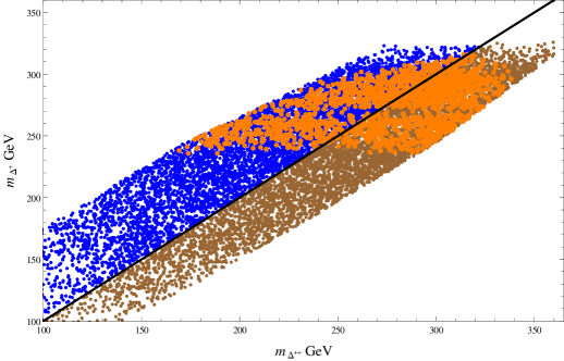
Figure 3: Correlation between $m_{\Delta^{++}}$ and $m_{\Delta^{+}}$. We have scanned the parameter space: $M\in(10,150)$ GeV, $\alpha\in(0,3)$, $\lambda_{2,3}\in(0,0.01)$ and $|\beta|\in(0,2)$. Here for $\beta<0$ (brown points) we have $m_{\Delta^{0}}<m_{\Delta^{+}}<m_{\Delta^{++}}$ and strong EWPhT region (orange points) lies for $m_{\Delta^{++}}\sim 250-340$ GeV. For $\beta>0$ (blue points) the mass hierarchy is opposite and strong EWPhT region (orange points) lies for $m_{\Delta^{++}}\sim 170-315$ GeV. In random scan, for $\beta>0$ and $\beta<0$, out of initial $10^{4}$ points, $8.54\%$ and $8.79\%$ points which are consistent with stability conditions and electroweak precision data (EWPD) showed strong EWPhT respectively. The straight line represents $m_{\Delta^{++}}=m_{\Delta^{+}}$.

In the above analysis, $Z_{2}$ symmetry is retained but one can introduce the term $\mu\Phi^{T}\epsilon\Delta^{\dagger}\Phi$ which breaks $Z_{2}$ symmetry softly, which happens in for example, type-II seesaw model. Such term will induce a triplet vev, $\langle\Delta^{0}\rangle=v_{\Delta}$ where $v_{\Delta}=\frac{\mu v^{2}}{\sqrt{2}M_{\Delta}^{2}}$. As indicated in [106], such term will modify the Higgs quartic coupling to $\frac{\lambda_{1}}{4}\rightarrow\frac{\lambda_{1}}{4}-\frac{\mu^{2}}{2M_{\Delta}^{2}}$ which in turn, will reduce the effective Higgs quartic coupling and enhance the strength of the transition. The upper bound of $v_{\Delta}$ set by precision measurement of $\rho$ parameter, is $2.5-4.6$ GeV [107] and lower bound is $10^{-10}$ GeV set by the neutrino mass [109]. Now from inequality (3.17), one can see that strong 1st order EWPhT favors $M_{\Delta}\leq T_{c}\sim 100-120$ GeV. Therefore $\mu$ will lie within the range $10^{-11}\leq\mu\leq 1.5$ GeV. Therefore the correction to the Higgs quartic coupling is about $O(10^{-3})$ so it is negligible and does not quantitatively change the transition which is mostly driven by large $\alpha$ coupling of the potential. Also correction to mass spectrum due to non zero $\mu$ term (therefore, nonzero $v_{\Delta}$) is $O(\frac{v_{\Delta}^{2}}{v^{2}})$ and thus very small. So EWPhT results obtained in $Z_{2}$ symmetric triplet case also holds for softly broken $Z_{2}$ symmetric model.

In [108], for like-sign dilepton final states with $100\%$ branching ratio at 7 TeV LHC run, the lower limit on mass of the doubly charged scalar was put as 409 GeV, 398 GeV and 375 GeV for $e^{\pm}e^{\pm}$, $\mu^{\pm}\mu^{\pm}$ and $e^{\pm}\mu^{\pm}$ final states. But as pointed out in [109] the mass limit crucially depends on the value of $v_{\Delta}$ and the di-leptonic decay channel $\Gamma_{\Delta^{++}\rightarrow l_{i}l_{j}}$ is dominant only when $10^{-10}\leq v_{\Delta}\leq 10^{-5}-10^{-4}$ GeV and when $v_{\Delta}=10^{-4}-10^{-3}$ it becomes comparable to $\Gamma_{\Delta^{++}\rightarrow W^{+}W^{+}}$. Also for mass difference $\Delta M=m_{\Delta^{++}}-m_{\Delta^{+}}\geq 5$ GeV and $v_{\Delta}\geq 10^{-4}$ GeV, cascade decay is the most dominant decay channel ($\beta<0$). Therefore when $v_{\Delta}\sim 4\times 10^{-5}$ GeV, di-leptonic branching ratio is around $11\%$ and lower limits on $m_{\Delta^{++}}$ are 212 GeV ($e^{+}e^{+}$), 216 GeV ($\mu^{+}\mu^{+}$) and 190 GeV ($e^{+}\mu^{+}$) which is still compatible with strong EWPhT region shown in Fig.(3). Moreover, for $v_{\Delta}\geq 10^{-4}$ the limit goes down all the way to $m_{\Delta^{++}}\geq 100$ GeV and thus again compatible with strong EWPhT region.

Quartet Representation

In case of quartet representation, the thermal mass for the Higgs and Goldstone fields are

$$m_{h}^{2}(\phi,T)=-\mu^{2}+3\lambda_{1}\phi^{2}+a_{q}\frac{T^{2}}{12}$$ (3.26)

$$m^{2}_{G^{\pm}}=m^{2}_{G^{0}}=-\mu^{2}+\lambda_{1}\phi^{2}+a_{q}\frac{T^{2}}{12}$$ (3.27)

And for quartet, the thermal mass for the component fields are

$$m_{S}^{2}(\phi,T) = M_{Q}^{2}+\frac{1}{2}(\alpha+\frac{1}{4}\beta-2\gamma)\phi^{2}+b_{q}\frac{T^{2}}{12}$$ (3.28)

$$m_{A}^{2}(\phi,T) = M_{Q}^{2}+\frac{1}{2}(\alpha+\frac{1}{4}\beta+2\gamma)\phi^{2}+b_{q}\frac{T^{2}}{12}$$ (3.29)

$$m_{Q^{++}}^{2}(\phi,T) = M_{Q}^{2}+\frac{1}{2}(\alpha-\frac{3}{4}\beta)\phi^{2}+b_{q}\frac{T^{2}}{12}$$ (3.30)

$$m_{Q_{1}^{+}}^{2}(\phi,T) = M_{Q}^{2}+\frac{1}{2}(\alpha+\frac{1}{4}\beta-\frac{1}{2}\sqrt{\beta^{2}+12\gamma^{2}})\phi^{2}+b_{q}\frac{T^{2}}{12}$$ (3.31)

$$m_{Q_{2}^{+}}^{2}(\phi,T) = M_{Q}^{2}+\frac{1}{2}(\alpha+\frac{1}{4}\beta+\frac{1}{2}\sqrt{\beta^{2}+12\gamma^{2}})\phi^{2}+b_{q}\frac{T^{2}}{12}$$ (3.32)

Here the thermal coefficient $a_{q}$ and $b_{q}$ are,

$$a_{q} = 6\lambda_{1}+4\alpha+\frac{9}{4}g^{2}+\frac{3}{4}g^{\prime 2}+3y_{t}^{2}$$ (3.33)

$$b_{q} = 10\lambda_{2}+\frac{15}{2}\lambda_{3}+2\alpha+\frac{45}{4}g^{2}+\frac{3}{4}g^{\prime 2}$$ (3.34)

Similarly the thermal potential is

$$V_{eff}(\phi,T) = \frac{1}{2}(-\mu^{2}+a_{q}\frac{T^{2}}{12})\phi^{2}+\frac{\lambda_{1}}{4}\phi^{4}+\sum_{i}(\pm)g_{i}\frac{m_{i}(\phi)^{4}}{64\pi^{2}}[\ln\frac{m^{2}_{i}(\phi)}{Q^{2}}-c_{i}]$$

$$- \frac{T}{12\pi}\sum_{B}g_{B}[m^{2}_{B}(\phi,T)]^{3/2}-\sum_{B}\frac{m^{4}_{B}(\phi,T)}{64\pi^{2}}\ln\frac{m^{2}_{B}(\phi,T)}{A_{b}T^{2}}$$

$$+ 12\frac{m^{4}_{t}(\phi)}{64\pi^{2}}\ln\frac{m^{2}_{t}(\phi)}{A_{f}T^{2}}$$

where bosonic sum is taken over, $h$, $G^{\pm}$, $G^{0}$, $Q^{++}$, $Q_{1}^{+}$, $Q_{2}^{+}$, $S$, $A$, $W^{\pm}$ and $Z$ with corresponding degrees of freedom, $\{h,G^{\pm},G^{0},Q^{++},Q_{1}^{+},Q_{2}^{+},S,A,W^{\pm},Z,t\}=\{1,2,1,2,2,2,1,1,6,3,12\}$.

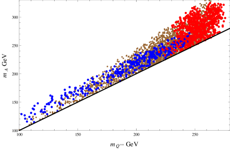
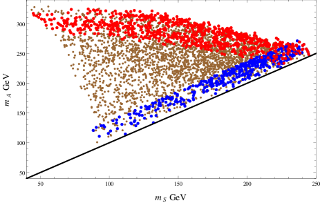
Figure 4: Correlation between (left fig.) $m_{Q^{++}}$ and $m_{A}$ and (right fig.) $m_{S}$ and $m_{A}$. We have scanned the parameter space: $M\in(0,60)$ GeV, $\lambda_{2,3}\in(0,0.01)$, $\alpha\in(0,2)$, $|\beta|\in(0,1.5)$ and $\gamma\in(0,1.5)$. Out of initial $10^{5}$ models, for $\beta>0$ (blue points in left and right fig.), $0.43\%$ points satisfy stability conditions + precision data and mass hierarchy when considering $S$ to be dark matter where as for $\beta<0$ (brown points in both fig.), $3.47\%$ points satisfy the same bounds. In addition, for $\beta>0$ and $\beta<0$, strong EWPhT condition (red points in both figures) is satisfied by $0.04\%$ points with $m_{Q^{++}}\sim 200-250$ GeV and $m_{A}\sim 230-270$ and $0.8\%$ points with $m_{Q^{++}}\sim 230-275$ GeV and $m_{A}\sim 235-320$ respectively. The straight line in left fig. represents $m_{Q^{++}}=m_{A}$ and in right fig., $m_{S}=m_{A}$.

Expansion Parameter

One also has to keep in mind the validity of finite temperature perturbation expansion. In case of standard model, the first order phase transition is dominated by the gauge bosons but for the case of (previously considered) inert doublet, complex triplet or quartet, the phase transition is mainly driven by new scalar couplings to the Higgs. Therefore, we can safely neglect the gauge boson contribution. As an illustration, we can see by simplifying Eq.(3.9) and Eq.(3.2) that if the effective scalar coupling, $\alpha_{S}$ is responsible for the transition, in the region near the symmetry breaking minimum, $\phi/T\sim\alpha_{S}^{3/2}/\lambda_{1}$. The thermal mass of the corresponding particle is,

$$m^{2}_{S}(\phi,T)=M^{2}+\frac{1}{2}\alpha_{S}\phi^{2}+\Pi(T)$$ (3.36)

Additional loop containing scalar will cost a factor $\sim\alpha_{S}T$ and loop expansion parameter can be obtained by dividing this factor with the leading mass of the theory which in this case is the mass of the new scalar; $\beta\sim\frac{\alpha_{S}T}{m_{S}}$. Now only in the limit, $M^{2}+\Pi(T)<<\alpha_{S}\phi^{2}$, we have, $\beta\sim\sqrt{\alpha_{S}}\frac{T}{\phi}$ or, near the region of minimum, $\beta\sim\frac{\lambda_{1}}{\alpha_{S}}\sim\frac{m^{2}_{h}}{m^{2}_{S}}$. Therefore, perturbation makes sense only for $\lambda_{1}<\alpha_{S}$ or $m_{h}<m_{S}$. On the other hand if $M^{2}+\Pi(T)$ term is significantly larger, it will reduce the order parameter and eventually transition will cease to be first order. In case of complex triplet, from Fig.(3), the 1st order EWPhT occurs for region: $m_{\Delta^{++}}\sim 170-340$ GeV. And for quartet, from Fig.(4), first order EWPhT region is: $m_{Q^{++}}\sim 200-275$ GeV and $m_{A}\sim 230-320$ GeV. Therefore we can see that for both cases, the mass regions where first order transition occurs are larger than the Higgs mass and hence, within the validity of perturbation theory.

3.3 Impact of Multiplets’ Sizes on EWPhT

Latent Heat Release

The phase transition is characterized by the release of latent heat. If there is a latent heat release, the transition is first order in nature otherwise it is second or higher order (as in Ehrenfest’s classification). The nature of cosmological phase transition is addressed in [110, 111]. In this section, we have addressed how the size of the representation affects the latent heat release during the electroweak phase transition with assumption that the transition is first order driven by large Higgs-inert scalar coupling, i.e. $\alpha$. Consider a system gone through first order phase transition at temperature, $T_{c}$. The high temperature phase consists of radiation energy and false vacuum energy and energy density is denoted as $\rho_{+}$. On the other hand, although low temperature phase has equal free energy $F$ it will have different energy density, $\rho_{-}$. The discontinuity $\Delta\rho(T_{c})=\rho_{+}(T_{c})-\rho_{-}(T_{c})$, gives the latent heat, $L=\Delta\rho(T_{c})=T_{c}\Delta s(T_{c})$ where $\Delta s(T_{c})=s_{+}-s_{-}$ is entropy density difference and it is liberated when the region of high-T phase is converted into the low-T phase. Therefore, using $F=\rho-Ts$ with $s=-\frac{dF}{dT}$ and from expression for effective potential (equivalent to free energy), Eq.(3.2) and as for 1st order phase transition, $F_{+}(0,T_{c})=F_{-}(\phi_{c},T_{c})$, we have the latent heat for the transition,

$$L=T\frac{dF_{-}}{dT}|_{(\phi_{c},T_{c})}-T\frac{dF_{+}}{dT}|_{(0,T_{c})}$$ (3.37)

For simplicity we can again take real degenerate representation for probing the impact of dimension of large multiplet on the latent heat release. As the amount of latent heat represents the strength of first order transition, it is already clear from Fig.(5) that larger representation disfavors first order phase transition. In addition, in Sec.(2.3) we have seen that arbitrarily large scalar multiplet makes gauge and scalar couplings non-perturbative in TeV or even at smaller scale. Therefore, larger scalar multiplet cannot simultaneously strengthen the electroweak phase transition and stay consistent with perturbativity and unitarity of the theory. Similar conclusion can be drawn for complex even integer and half integer multiplets.

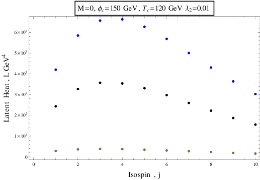
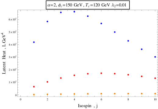
Figure 5: In the left graph, latent heat decreases when isospin increases; blue, black and brown dots represents $\alpha=$2, $1$ and $0.1$ respectively. On the right, we can see again the reduction of latent heat with isospin for invariant mass term, $M=0$ (blue), $500$ (red) and $1000$ (orange) GeV respectively.

4 The Quartet/Doublet versus EW, EWPhT and CDM Constraints.

In this section, we have tried to identify region of parameter space for higher representations where one can have light DM candidate consistent with other phenomenological constraints along with strong EWPhT. As already pointed out in Sec.(2.2), DM of complex even integer multiplet ($Y\neq 0$) is excluded by the bound from direct detection. On the other hand, the $\gamma$ term of Eq.(2.1) can split the neutral component of half integer representation and one can easily obtain a light DM component. As quartet multiplet $(j=3/2)$ is the immediate generalization of inert doublet, we focused on identifying DM properties in parallel with it’s impact on Strong EWPhT.

4.1 Model Parameters Scan and Constraints

The masses of quartet’s component fields are determined by four free parameters $\{M_{Q},\alpha,\beta,\gamma\}$, Eq.(2.2). But (co)annihilation cross sections which control the relic density of the dark matter depend on the mass splittings among dark matter and the others components in the multiplet. Therefore we used alternative free parameter set $\{m_{S},\lambda_{S},m_{Q^{++}},m_{A}\}$ where $m_{S}$ is the DM mass and $\lambda_{S}=\alpha+\frac{1}{4}\beta-2\gamma$ is the coupling between between Higgs and dark matter component. One can express $\{M_{Q},\alpha,\beta,\gamma,m_{Q^{+}_{1}},m_{Q^{+}_{2}}\}$ in terms of these four parameters using mass relations Eq.(2.2). Moreover, in case of quartet, for $S$ to be the lightest component of the multiplet, one needs to impose two conditions, $\gamma>0$ and $\gamma\geq\frac{|\beta|}{2}$ which in turn sets the mass spectrum to be $m_{S}<m_{Q^{+}_{1}}<m_{Q^{++}}<m_{Q^{+}_{2}}<m_{A}$.

Collider Constraints:
Direct collider searches at LEP II has put a strong bound on single charged particle which is $m_{Q^{+}_{1}}>70-90$ GeV [113]. But the doubly charged scalar of the quartet which only has the cascade decay channel is not strongly constrained by collider searches. One constraint can come from $W$ and $Z$ boson width. In our case, setting $S$ as DM imposes in the mass spectrum: $m_{Q^{++}}\geq m_{Q^{+}_{1}}$ so the constraint on single charged scalar is also translated into a bound on the doubly charged scalar for such mass spectrum. Moreover, the deviations of $W$ and $Z$ width from their SM values can take place through decay channels: $W^{\pm}\rightarrow SQ^{\pm}_{1}/AQ^{\pm}_{1}/Q^{\pm\pm}Q^{\mp}_{1}$ and $Z\rightarrow Q^{+}_{1}Q^{-}_{1}/SA/Q^{++}Q^{--}$. Therefore to avoid such deviation the following mass constraints are also imposed: $m_{S}+m_{Q^{+}_{1}}>m_{W}$, $m_{A}+m_{Q^{+}_{1}}>m_{W}$, $m_{Q^{++}}+m_{Q^{+}_{1}}>m_{W}$, $m_{Q^{+}_{1}}>m_{Z}/2$, $m_{Q^{++}}>m_{Z}/2$ and $m_{S}+m_{A}>m_{Z}$. Apart from collider constraints, one also impose constraints coming from electroweak precision observables. In our scan, we used the allowed range of $T$ parameter, Eq.(2.25) and $S$ parameter, Eq.(2.27).

DM Relic Density Constraint:
The dark matter density of the universe measured by Planck collaboration is $\Omega_{DM}h^{2}=0.1196\pm 0.0031$ ($68\%$ CL) [114]. To determine the relic density of the multiplets, we used FeynRules [116] to generate the model files for MicrOMEGAs [120]. For inert multiplets, mass splitting between components are set by both $\beta$ and $\gamma$ couplings. In case of doublet, one can set $\beta$ and $\gamma$ to produce large spitting between $S$ component and single charged component $C^{+}$ or between $S$ and $A$ in such way that such splitting is compatible with electroweak precision observables. Such large splitting can lead to suppression of co-annihilation channels $SA,SC^{+}\rightarrow$ SM particles. But such simple tuning of the couplings like in the doublet is not possible for quartet because of the mass relation Eq.(2.2). Therefore there is a possibility for co-annihilation channel to open up when $m_{Q^{+}_{1}}/m_{S}\leq 1.5$ ([115]).

Apart from co-annihilation, other dominant channels which will control the relic density of DM at the low mass region are $SS\rightarrow h^{*}\rightarrow b\bar{b}$ and $SS\rightarrow WW$.

Direct DM Detection and Invisible Higgs Decay Constraints:
There is also a strict limit on the spin independent DM-nucleon cross section coming from direct detection experiment. The spin independent cross section is given by,

$$\sigma_{SI}=\frac{\lambda_{S}^{2}f^{2}}{4\pi}\frac{\mu^{2}m^{2}_{n}}{m^{4}_{h}m^{2}_{S}}$$ (4.1)

Here, $\mu=m_{n}m_{s}/(m_{n}+m_{s})$ is the DM-nucleon reduced mass. $f$ parameterizes the nuclear matrix element, $\sum_{u,d,s,c,b,t}\langle n|m_{q}\bar{q}q|n\rangle\equiv fm_{n}\bar{n}{n}$ and from recent lattice results [117], $f=0.347131$. Now XENON100 with 225 days live data [118] sets bound on cross section to be $\sigma_{SI}\lesssim 2\times 10^{-45}\text{cm}^{2}$. In addition, the future XENON1T will reach the sensitivity of $\sigma_{SI}\lesssim 2\times 10^{-47}\text{cm}^{2}$ [119].

Also if the mass of the dark matter is smaller than half of the Higgs mass, it will contribute to the invisible decay of the Higgs through $h\rightarrow SS$ with branching ratio $Br_{\text{inv}}=\Gamma_{\text{inv}}/(\Gamma_{\text{SM}}+\Gamma_{\text{inv}})$, where $\Gamma_{\text{SM}}=6.1$ MeV and,

$$\Gamma_{inv}=\frac{\lambda_{S}^{2}v^{2}}{64\pi m_{h}}\sqrt{1-\frac{4m_{S}^{2}}{m_{h}^{2}}}$$ (4.2)

Consequently, current limit on the branching ratio for Higgs invisible decay [112] will constrain the $\lambda_{S}$ coupling. However, note that as can be seen in Fig.(6), the limit imposed on $\lambda_{S}$ by XENON100 is more stringent than the limit coming from invisible Higgs decay for mass range $45\leq m_{S}\leq 63$ GeV.

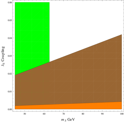
Figure 6: The region in $m_{S}-\lambda_{S}$ plane allowed by invisible branching ratio limit $Br_{inv}\leq 0.65$ (green region) and XENON100 limit (brown region) and XENON1T limit (orange region) respectively for DM mass range $45\leq m_{S}\leq 100$ GeV. The future XENON1T will significantly reduce the allowed region down to $0.002\lesssim\lambda_{S}\lesssim 0.004$ for $m_{S}=45-100$ GeV.

4.2 Allowed Parameter Regions

To determine allowed parameter region for quartet and compare it with inert doublet case, we used dark matter relic density constraint at $5\sigma$ to take into account all the numerical uncertainties. For numerical scanning, we considered the following range: $m_{S}\in(45,100)$ GeV, $\lambda_{S}\in(0.001,0.02)$, $m_{Q^{++}}\in(100,350)$ GeV and $m_{A}\in(100,350)$ GeV for both doublet and quartet case.

At low mass region $(m_{S}\leq m_{W})$ the dominant annihilation channel is $SS\rightarrow h^{*}\rightarrow b\bar{b}$. When the mass becomes larger than $m_{W}$ and $m_{Z}$, $SS\rightarrow W^{+}W^{-}$ and $SS\rightarrow ZZ$ open up and dominate the annihilation rate. Therefore the relic density becomes much lower than the observed relic density. Subsequent increase of $m_{S}$ will open up $SS\rightarrow hh$ and $SS\rightarrow t\bar{t}$ which will dominate along with $WW$ and $ZZ$ annihilation channels and eventually the relic density will be much smaller than observed value. Inert doublet has already shown such behavior [36, 27].

From scatter plot, Fig.(7) we can see that, unlike the doublet case, for quartet, the parameter space allowing both light DM consistent with observed relic density and strong first order phase transition is hard to achieve. Out of an initial of $10^{5}$ models, for doublet, $20\%$ are consistent with stability conditions + precision data+ collider constraints, $0.77\%$ satisfy, in addition, the EWPhT condition $\phi_{c}/T_{c}\geq 1$ and $0.234\%$ agree with the observed $\Omega_{DM}h^{2}$ at $5\sigma$, DM direct detection bounds and invisible Higgs decay limits. Only $0.02\%$ of the initial models survive all the constraints. In contrast, for quartet, from an initial of $10^{5}$ models only $2\%$ satisfy stability conditions + EWPD +collider constraints, $0.13\%$ points satisfy additional strong EWPhT condition and only $0.03\%$ models, observed $\Omega_{DM}h^{2}$ at $5\sigma$ and direct detection bounds. Lastly, only $0.003\%$ models satisfied all the conditions. Therefore, in case of providing strong EWPhT with a light dark matter, quartet is disfavored with respect to doublet.

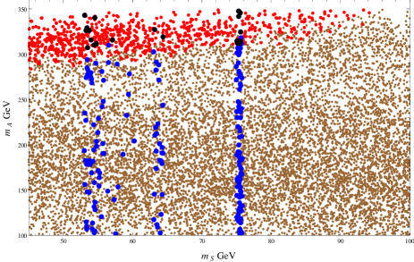
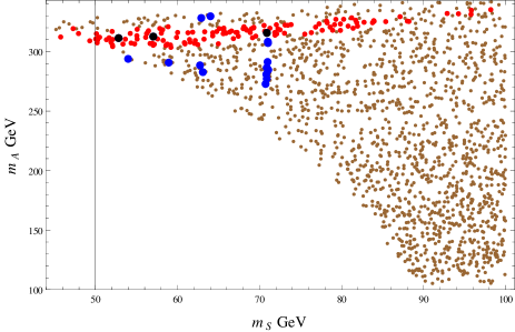
Figure 7: Scatter plot representing the correlation between $m_{S}$ and $m_{A}$ for doublet(left fig.) and quartet (right fig.). Brown points represent models satisfying stability conditions + precision bounds+collider constraints. Red points correspond to models also satisfying the EWPhT condition $\phi_{c}/T_{c}\geq 1$ and blue points correspond to models consistent only with observed relic density at $5\sigma$ and DM direct detection and invisible Higgs decay bounds. Black points are models consistent with stability conditions + EWPD + collider constraints + the EWPhT condition $\phi_{c}/T_{c}\geq 1$ + observed $\Omega_{DM}h^{2}$ + DM direct detection and invisible Higgs decay limits.

5 Conclusions and outlook

We have considered the electroweak phase transition and dark matter phenomenology with various inert scalar representations used for extending the SM’s Higgs sector. The details of the phenomenological studies are done by making random scans of parameters within the triplet and quartet context. The results from our analyses in comparing the allowed parameter regions of the above mentioned models with the inert doublet model case are summarized as follows

• As the size of an inert multiplet which can be added to the SM is not arbitrary but is rather controlled by the perturbativity of SU(2) gauge coupling at TeV scale ($\sim 10$ TeV), which sets an upper bound on the size of the multiplet to be $j\leq 5$, that motivated us to study the EWPhT (and subsequently, the DM characteristics) for the triplet and quartet models as representatives for allowed larger multiplets. We explicitly showed that it is possible to have strong EWPhT within the complex inert triplet and the inert quartet models. In case of complex triplet, from Fig.(3), the 1st order EWPhT occurs for region: $m_{\Delta^{++}}\sim 170-340$ GeV. And for quartet, from Fig.(4), first order EWPhT region is: $m_{Q^{++}}\sim 200-275$ GeV and $m_{A}\sim 230-320$ GeV as compared to the mass of inert doublet’s singly charged component, $m_{C}$ ($\sim$ pseudo-scalar component’s mass, $m_{A}$) in $270-350$ GeV [19].

• Using the expression for the latent heat measure, we have made a generic study of the impact of higher (than the doublet) scalar multiplets on the strength of electroweak phase transition. The compete between the number of scalar quasiparticles coupled to EW plasma with large couplings and the screening of those particles resulting from scalar self quartic and gauge boson interaction, which will decouple them from the plasma, determines the strength of the transition. The rise and fall of the latent heat with large multiplet, as shown in Fig.(5), qualitatively shows such variation of the EWPhT strength.

• Next we require the simultaneous explanation of EWPhT and the cold DM content of the universe within the quartet frame. The triplet with $Y=2$, unlike the half integer representations, is already excluded by the direct detection limit thus can’t play any viable role of DM triggering strong EWPhT. Therefore for quartet, we identified the region of parameter space, out of the randomly scanned parameter points, which allows both strong EWPhT and a light DM candidate by imposing stability conditions, electroweak precision bounds and corresponding experimental limits. The parameter regions that survive all constraints imposed are compared with similar results from within the inert doublet frame. Requiring that all the CDM content of the universe is explained by the scalar multiplet then, from the scatter plot Fig.(7), it can be seen that the quartet has only a very small allowed parameter space in contrast to inert doublet case. Moreover, the allowed parameter space for having DM with observed relic density and strong EWPhT in both inert doublet and quartet cases will be significantly constrained by future XENON1T experiment.

The above results combined together point out that the higher inert representations are rather disfavored compared to the inert doublet. The conclusion is qualitative and only valid within the set of experimental and phenomenological constrains considered. There are however room for doing more in directions we did not consider here:

• The computational and phenomenological machineries are well within reach for making detailed quantitative analyses within Bayesian statistical framework. Using strong EWPhT condition and recent results from relic density measurement, direct and indirect detection limits and collider constraints from LHC, a comparison between the allowed parameter spaces of inert doublet and quartet can be carried out in this Bayesian framework, in a similar manner to the work done for comparing different supersymmetric models [121, 122] and for comparing a single versus multi-particle CDM universe hypotheses [123].

• Higher (than doublet) scalar multiplets have relatively more charged components that couple to the Higgs. As such, they will alter the decay rate of Higgs going to two photons relative to the SM value [124, 125, 126, 127, 128, 129]. Persistence of the apparent (given the large uncertainties) excess in the $h\rightarrow\gamma\gamma$ data will severely constrain the triplet and quartet parameter regions with EWPhT driven by large positive couplings [130, 131]. This and similar studies will be interesting for establishing the inert multiplets’ status and/or prospects within collider phenomenology framework.

Acknowledgements:

T.A.C. is deeply indebted to Goran Senjanović for the suggestion to investigate larger scalar multiplets and the guidance in every step of the work. T.A.C. is also grateful to Yue Zhang and Miha Nemevšek for many helpful discussions and Amine Ahriche for careful reading of the manuscript. T.A.C. would also like to thank Andrea de Simone, Marco Serone, Gabrijela Zaharijas, Abdesslam Arhrib, Rachik Soualah, Muhammad Muteeb Nouman and Arshad Momen for helpful comments and discussions.

6 Appendix

6.1 Quartet $SU(2)$ Representation Generators

The generators $R(T^{a})$ in representation $R$ of $SU(2)$ are taken in such a way that they satisfy the following relation: $Tr[R(T^{a})R(T^{b})]=T(R)\delta^{ab}.$ Here $T(R)$ is the dynkin index for the corresponding representation. It is obtained from $T(R)D(Ad)=C(R)D(R)$ where dimension of Adjoint reps. is $D(Ad)=3$ for $SU(2)$ and Casimir invariant is $\sum_{a}R(T^{a})R(T^{a})=j(j+1)$ and dimension of the reps. $R$ is $D(R)=2j+1$. For $SU(2)$ reps. $T(\frac{1}{2})=\frac{1}{2}$ and $T(\frac{3}{2})=5$.

The explicit form of the generators for quartet reps are the following:

$$T^{1}=\begin{pmatrix}0&\frac{\sqrt{3}}{2}&0&0\\ \frac{\sqrt{3}}{2}&0&1&0\\ 0&1&0&\frac{\sqrt{3}}{2}\\ 0&0&\frac{\sqrt{3}}{2}&0\\ \end{pmatrix}\,,\quad T^{2}=\begin{pmatrix}0&-\frac{\sqrt{3}i}{2}&0&0\\ \frac{\sqrt{3}i}{2}&0&-i&0\\ 0&i&0&-\frac{\sqrt{3}i}{2}\\ 0&0&\frac{\sqrt{3}i}{2}&0\\ \end{pmatrix}\,,\quad T^{3}=\text{diag}(\frac{3}{2},\frac{1}{2},-\frac{1}{2},-\frac{3}{2}).$$ (6.1)

The raising and lowering operators are defined as $T^{\pm}=T^{1}\pm iT^{2}$. The antisymmetric matrices in doublet reps is $\epsilon$ and the similar antisymmetric matrix for quartet representation, $C$ is constructed using the relation $CT^{a}C^{-1}=-T^{aT}$ because the explicit form of it depends on the matrix representation of the corresponding generators:

$$\epsilon=\begin{pmatrix}0&1\\ -1&0\\ \end{pmatrix}\,,\quad C=\begin{pmatrix}0&0&0&1\\ 0&0&-1&0\\ 0&1&0&0\\ -1&0&0&0\end{pmatrix}$$ (6.2)

6.2 High Temperature Expansion of Thermal Potential

The finite temperature effective potential is

$$V_{T} = \sum_{B(F)}(\pm)g_{B(F)}\frac{T^{4}}{2\pi^{2}}\int_{0}^{\infty}dxx^{2}\ln(1\mp e^{-\sqrt{x^{2}+m_{B(F)}^{2}(\phi_{i},T)/T^{2}}})$$ (6.3)

$$= \sum_{B(F)}(\pm)g_{B(F)}\frac{T^{4}}{2\pi^{2}}J_{B(F)}(m_{B(F)}^{2}(\phi_{i},T)/T^{2})$$

where, $J_{B}(m^{2}_{B}/T^{2})$ and $J_{F}(m^{2}_{F}/T^{2})$ are denoting bosonic and fermionic integral respectively.

In the High temperature limit, $m(\phi)/T<1$, finite temperature bosonic integral is

$$J_{B}(\frac{m^{2}}{T^{2}}) = \int_{0}^{\infty}dxx^{2}\ln(1-e^{-\sqrt{x^{2}+m^{2}/T^{2}}})=-\frac{\pi^{4}}{45}+\frac{\pi^{2}}{12}\frac{m^{2}}{T^{2}}-\frac{\pi}{6}(\frac{m^{2}}{T^{2}})^{\frac{3}{2}}-\frac{1}{32}\frac{m^{4}}{T^{4}}\ln\frac{m^{2}}{A_{b}T^{2}}$$

$$- 2\pi^{\frac{7}{2}}\sum_{l=1}^{\infty}(-1)^{l}\frac{\zeta(2l+1)}{(l+1)!}\Gamma(l+\frac{1}{2})(\frac{m^{2}}{4\pi^{2}T^{2}})^{l+2}\quad\textrm{where }\,A_{b}=16\pi^{2}e^{(3/2-2\gamma_{E})}(\ln A_{b}=5.4076),$$

$\gamma_{E}$ is Euler’s constant and $\zeta$ is the Riemann $\zeta$-function. The fermionic integral is

$$J_{F}(\frac{m^{2}}{T^{2}})=\int_{0}^{\infty}dxx^{2}\ln(1+e^{-\sqrt{x^{2}+m^{2}/T^{2}}})=-\frac{7\pi^{4}}{360}+\frac{\pi^{2}}{24}\frac{m^{2}}{T^{2}}-\frac{1}{32}\frac{m^{4}}{T^{4}}\ln\frac{m^{2}}{A_{f}T^{2}}$$

$$- \frac{\pi^{\frac{7}{2}}}{4}\sum_{l=1}^{\infty}(-1)^{l}\frac{\zeta(2l+1)}{(l+1)!}(1-2^{-2l-1})\Gamma(l+\frac{1}{2})(\frac{m^{2}}{4\pi^{2}T^{2}})^{l+2}\quad\textrm{where }\,A_{f}=\pi^{2}e^{(3/2-2\gamma_{E})}(\ln A_{b}=2.6351).$$

6.3 Renormalization Group Equations

The doublet RG equations [25] in our parameterization are in the following. Here $g_{2}$, $g_{Y}$ and $g_{3}$ are $SU(2)_{L}$, $U(1)_{Y}$ and $SU(3)_{c}$ couplings respectively.

$$16\pi^{2}\beta_{\lambda_{1}} = 24\lambda_{1}^{2}+2\alpha^{2}+\frac{1}{8}\beta^{2}+\gamma^{2}-9\lambda_{1}g_{2}^{2}-3\lambda_{1}g_{Y}^{2}+\frac{9}{4}g_{2}^{4}+\frac{3}{4}g_{Y}^{4}+\frac{3}{2}g_{2}^{2}g_{Y}^{2}+12\lambda_{1}y_{t}^{2}-6y_{t}^{4}$$

$$16\pi^{2}\beta_{\lambda_{2}} = 24\lambda_{2}^{2}+2\alpha^{2}+\frac{1}{8}\beta^{2}+\gamma^{2}-9\lambda_{2}g_{2}^{2}-3\lambda_{2}g_{Y}^{2}+\frac{9}{4}g_{2}^{4}+\frac{3}{4}g_{Y}^{4}+\frac{3}{2}g_{2}^{2}g_{Y}^{2}$$

$$16\pi^{2}\beta_{\alpha} = 4\alpha^{2}+12\lambda_{1}\alpha+\lambda_{2}\alpha+\frac{3}{4}\beta^{2}+6\gamma^{2}-9\alpha g_{2}^{2}-\alpha g_{Y}^{2}+\frac{9}{4}g_{2}^{4}+\frac{3}{4}g_{Y}^{4}-\frac{3}{2}g_{2}^{2}g_{Y}^{2}+12\alpha y_{t}^{2}$$

$$16\pi^{2}\beta_{\beta} = 4\lambda_{1}\beta+4\lambda_{2}\beta+8\alpha\beta+16\gamma^{2}-9\beta g_{2}^{2}-\beta g_{Y}^{2}+12\beta y_{t}^{2}$$

$$16\pi^{2}\beta_{\gamma} = 4\lambda_{1}\gamma+4\lambda_{2}\gamma+8\alpha\gamma+4\beta\gamma-9\gamma g_{2}^{2}-\gamma g_{Y}^{2}+12\gamma y_{t}^{2}$$

$$16\pi^{2}\beta_{g_{2}} = -3g_{2}^{3},\,\,\,16\pi^{2}\beta_{g_{Y}}=\frac{22}{3}g_{Y}^{3},\,\,\,16\pi^{2}\beta_{g_{3}}=-7g_{3}^{3}$$

$$16\pi^{2}\beta_{y_{t}} = y_{t}(\frac{9}{2}y_{t}^{2}-\frac{17}{12}g_{Y}^{2}-\frac{9}{4}g_{2}^{2}-8g_{3}^{2})$$ (6.6)

And the Triplet RG equations [75] relevant for our analysis are,

$$16\pi^{2}\beta_{\lambda_{1}} = 24\lambda_{1}^{2}+6\alpha^{2}+\beta^{2}-9\lambda_{1}g_{2}^{2}-3\lambda_{1}g_{Y}^{2}+\frac{9}{2}g_{2}^{4}+\frac{3}{2}g_{Y}^{4}+3g_{2}^{2}g_{Y}^{2}+12\lambda_{1}y_{t}^{2}-6y_{t}^{4}$$

$$16\pi^{2}\beta_{\lambda_{2}} = 28\lambda_{2}^{2}+48\lambda_{2}\lambda_{3}+24\lambda_{3}^{2}+2\alpha^{2}+\beta^{2}-24\lambda_{2}g_{2}^{2}-12\lambda_{2}g_{Y}^{2}+6g_{2}^{4}+6g_{Y}^{4}+24g_{2}^{2}g_{Y}^{2}$$

$$16\pi^{2}\beta_{\lambda_{3}} = 36\lambda_{3}^{2}+24\lambda_{2}\lambda_{3}-\frac{1}{2}\beta^{2}-24\lambda_{3}g_{2}^{2}-12\lambda_{3}g_{Y}^{2}+3g_{2}^{4}-12g_{2}^{2}g_{Y}^{2}$$

$$16\pi^{2}\beta_{\alpha} = 3\alpha^{2}+6\lambda_{1}\alpha+16\lambda_{2}\alpha+24\lambda_{3}\alpha-\frac{33}{2}\alpha g_{2}^{2}-\frac{15}{2}\alpha g_{Y}^{2}+6g_{2}^{4}+3g_{Y}^{4}+12y_{t}^{2}\alpha$$

$$16\pi^{2}\beta_{\beta} = 2\lambda_{1}\beta+4\lambda_{2}\beta-4\lambda_{3}\beta+16\alpha\beta-\frac{33}{2}\beta g_{2}^{2}-\frac{15}{2}\beta g_{Y}^{2}+12g_{2}^{2}g_{Y}^{2}-6\beta y_{t}^{2}$$

$$16\pi^{2}\beta_{g_{2}} = -\frac{5}{2}g_{2}^{3},\,\,\,16\pi^{2}\beta_{g_{Y}}=\frac{47}{6}\sqrt{\frac{5}{3}}g_{Y}^{3},\,\,\,16\pi^{2}\beta_{g_{3}}=-7g_{3}^{3}$$

$$16\pi^{2}\beta_{y_{t}} = y_{t}(\frac{9}{2}y_{t}^{2}-\frac{17}{12}g_{Y}^{2}-\frac{9}{4}g_{2}^{2}-8g_{3}^{2})$$ (6.7)

References

- [1] G. Aad et al. [ATLAS Collaboration], “Observation of a new particle in the search for the Standard Model Higgs boson with the ATLAS detector at the LHC,” Phys. Lett. B 716 (2012) 1 [arXiv:1207.7214 [hep-ex]].
- [2] S. Chatrchyan et al. [CMS Collaboration], “Observation of a new boson at a mass of 125 GeV with the CMS experiment at the LHC,” Phys. Lett. B 716 (2012) 30 [arXiv:1207.7235 [hep-ex]].
- [3] R. J. Scherrer, M. S. Turner, Phys. Rev. D33, 1585 (1986).
- [4] A. D. Sakharov, Pisma Zh. Eksp. Teor. Fiz. 5, 32 (1967) [JETP Lett. 5, 24 (1967)].
- [5] V. A. Kuzmin, V. A. Rubakov and M. E. Shaposhnikov, Phys. Lett. B 155, 36 (1985).
- [6] F. R. Klinkhamer and N. S. Manton, Phys. Rev. D 30, 2212 (1984).
- [7] P. B. Arnold and L. D. McLerran, Phys. Rev. D 36, 581 (1987).
- [8] M. Dine, P. Huet and R. L. Singleton, Jr, Nucl. Phys. B 375, 625 (1992).
- [9] G. W. Anderson and L. J. Hall, Phys. Rev. D 45, 2685 (1992).
- [10] M. Dine, R. G. Leigh, P. Y. Huet, A. D. Linde and D. A. Linde, Phys. Rev. D 46, 550 (1992) [hep-ph/9203203].
- [11] M. E. Shaposhnikov, Nucl. Phys. B 287, 757 (1987).
- [12] A. I. Bochkarev and M. E. Shaposhnikov, Mod. Phys. Lett. A 2, 417 (1987).
- [13] M. E. Shaposhnikov, Nucl. Phys. B 299, 797 (1988).
- [14] A. I. Bochkarev, S. V. Kuzmin and M. E. Shaposhnikov, Phys. Lett. B 244, 275 (1990).
- [15] K. Kajantie, M. Laine, K. Rummukainen and M. E. Shaposhnikov, Nucl. Phys. B 466, 189 (1996) [hep-lat/9510020].
- [16] K. Kajantie, M. Laine, K. Rummukainen and M. E. Shaposhnikov, Phys. Rev. Lett. 77, 2887 (1996) [hep-ph/9605288].
- [17] K. Kajantie, M. Laine, K. Rummukainen and M. E. Shaposhnikov, Nucl. Phys. B 493, 413 (1997) [hep-lat/9612006].
- [18] http://lephiggs.web.cern.ch/LEPHIGGS/papers/CERN-EP-98-046
- [19] T. A. Chowdhury, M. Nemevšek, G. Senjanović and Y. Zhang, JCAP 1202, 029 (2012) [arXiv:1110.5334 [hep-ph]].
- [20] D. Borah and J. M. Cline, Phys. Rev. D 86, 055001 (2012) [arXiv:1204.4722 [hep-ph]].
- [21] G. Gil, P. Chankowski and M. Krawczyk, Phys. Lett. B 717, 396 (2012) [arXiv:1207.0084 [hep-ph]].
- [22] J. M. Cline and K. Kainulainen, Phys. Rev. D 87, 071701 (2013) [arXiv:1302.2614 [hep-ph]].
- [23] N. G. Deshpande and E. Ma, Phys. Rev. D 18, 2574 (1978).
- [24] E. Ma, Phys. Rev. D 73, 077301 (2006) [hep-ph/0601225].
- [25] R. Barbieri, L. J. Hall, V. S. Rychkov, Phys. Rev. D74, 015007 (2006). [hep-ph/0603188].
- [26] H. Martinez, A. Melfo, F. Nesti, G. Senjanović, Phys. Rev. Lett. 106, 191802 (2011). [arXiv:1101.3796 [hep-ph]].
- [27] A. Melfo, M. Nemevšek, F. Nesti, G. Senjanović, Y. Zhang, Phys. Rev. D84 (2011) 034009. [arXiv:1105.4611 [hep-ph]].
- [28] M. Gell-Mann, P. Ramond, R. Slansky, Rev. Mod. Phys. 50, 721 (1978).
- [29] F. Wilczek, A. Zee, Phys. Rev. D25, 553 (1982).
- [30] G. Senjanović, F. Wilczek, A. Zee, Phys. Lett. B141, 389 (1984).
- [31] J. Bagger, S. Dimopoulos, Nucl. Phys. B244, 247 (1984).
- [32] T. D. Lee, C. -N. Yang, Phys. Rev. 104, 254-258 (1956). [
- [33] L. Lopez Honorez, E. Nezri, J. F. Oliver and M. H. G. Tytgat, JCAP 0702, 028 (2007) [hep-ph/0612275].
- [34] S. Andreas, T. Hambye and M. H. G. Tytgat, JCAP 0810, 034 (2008) [arXiv:0808.0255 [hep-ph]].
- [35] T. Hambye and M. H. G. Tytgat, Phys. Lett. B 659, 651 (2008) [arXiv:0707.0633 [hep-ph]].
- [36] E. M. Dolle and S. Su, Phys. Rev. D 80, 055012 (2009) [arXiv:0906.1609 [hep-ph]].
- [37] L. Lopez Honorez and C. E. Yaguna, JCAP 1101, 002 (2011) [arXiv:1011.1411 [hep-ph]].
- [38] P. Agrawal, E. M. Dolle and C. A. Krenke, Phys. Rev. D 79, 015015 (2009) [arXiv:0811.1798 [hep-ph]].
- [39] S. Andreas, M. H. G. Tytgat and Q. Swillens, JCAP 0904, 004 (2009) [arXiv:0901.1750 [hep-ph]].
- [40] E. Nezri, M. H. G. Tytgat and G. Vertongen, JCAP 0904, 014 (2009) [arXiv:0901.2556 [hep-ph]].
- [41] Q. -H. Cao, E. Ma and G. Rajasekaran, Phys. Rev. D 76, 095011 (2007) [arXiv:0708.2939 [hep-ph]].
- [42] E. Lundstrom, M. Gustafsson and J. Edsjo, Phys. Rev. D 79, 035013 (2009) [arXiv:0810.3924 [hep-ph]].
- [43] E. Dolle, X. Miao, S. Su and B. Thomas, Phys. Rev. D 81, 035003 (2010) [arXiv:0909.3094 [hep-ph]].
- [44] M. Gustafsson, PoS CHARGED 2010, 030 (2010) [arXiv:1106.1719 [hep-ph]].
- [45] M. Gustafsson, S. Rydbeck, L. Lopez-Honorez and E. Lundstrom, Phys. Rev. D 86, 075019 (2012) [arXiv:1206.6316 [hep-ph]].
- [46] M. Aoki, S. Kanemura and H. Yokoya, Phys. Lett. B 725, 302 (2013) [arXiv:1303.6191 [hep-ph]].
- [47] A. Arhrib, Y. -L. S. Tsai, Q. Yuan and T. -C. Yuan, arXiv:1310.0358 [hep-ph].
- [48] I. F. Ginzburg, K. A. Kanishev, M. Krawczyk and D. Sokolowska, Phys. Rev. D 82, 123533 (2010) [arXiv:1009.4593 [hep-ph]].
- [49] M. Gustafsson, E. Lundstrom, L. Bergstrom and J. Edsjo, Phys. Rev. Lett. 99, 041301 (2007) [astro-ph/0703512 [ASTRO-PH]].
- [50] S. Profumo, M. J. Ramsey-Musolf and G. Shaughnessy, JHEP 0708, 010 (2007) [arXiv:0705.2425 [hep-ph]].
- [51] A. Ahriche, Phys. Rev. D 75, 083522 (2007) [hep-ph/0701192].
- [52] J. R. Espinosa, T. Konstandin, F. Riva, Nucl. Phys. B854 (2012) 592-630. [arXiv:1107.5441 [hep-ph]].
- [53] J. M. Cline and K. Kainulainen, JCAP 1301, 012 (2013) [arXiv:1210.4196 [hep-ph]].
- [54] J. M. Cline, K. Kainulainen, P. Scott and C. Weniger, arXiv:1306.4710 [hep-ph].
- [55] V. Barger, P. Langacker, M. McCaskey, M. Ramsey-Musolf and G. Shaughnessy, Phys. Rev. D 79, 015018 (2009) [arXiv:0811.0393 [hep-ph]].
- [56] M. Gonderinger, H. Lim and M. J. Ramsey-Musolf, Phys. Rev. D 86, 043511 (2012) [arXiv:1202.1316 [hep-ph]].
- [57] A. Ahriche and S. Nasri, Phys. Rev. D 85, 093007 (2012) [arXiv:1201.4614 [hep-ph]].
- [58] S. Das, P. J. Fox, A. Kumar, N. Weiner, JHEP 1011, 108 (2010). [arXiv:0910.1262 [hep-ph]];
- [59] M. Carena, N. R. Shah and C. E. M. Wagner, arXiv:1110.4378 [hep-ph].
- [60] A. Ahriche and S. Nasri, JCAP 1307, 035 (2013) [arXiv:1304.2055].
- [61] M. Cirelli, N. Fornengo, A. Strumia, Nucl. Phys. B753, 178-194 (2006). [hep-ph/0512090].
- [62] T. Hambye, F. -S. Ling, L. Lopez Honorez and J. Rocher, JHEP 0907, 090 (2009) [Erratum-ibid. 1005, 066 (2010)] [arXiv:0903.4010 [hep-ph]].
- [63] M. S. Carena, A. Megevand, M. Quiros and C. E. M. Wagner, Nucl. Phys. B 716, 319 (2005) [hep-ph/0410352].
- [64] H. Davoudiasl, I. Lewis and E. Ponton, arXiv:1211.3449 [hep-ph].
- [65] M. Taoso, G. Bertone and A. Masiero, JCAP 0803, 022 (2008) [arXiv:0711.4996 [astro-ph]].
- [66] T. Hambye, PoS IDM 2010, 098 (2011) [arXiv:1012.4587 [hep-ph]].
- [67] M. Gustafsson, T. Hambye and T. Scarna, Phys. Lett. B 724, 288 (2013) [arXiv:1303.4423 [hep-ph]].
- [68] K. Kannike, Eur. Phys. J. C 72, 2093 (2012) [arXiv:1205.3781 [hep-ph]].
- [69] M. Magg and C. Wetterich, Phys. Lett. B94 (1980) 61; G. Lazarides, Q. Shafi and C. Wetterich, Nucl. Phys. B181 (1981) 287; R.N. Mohapatra and G. Senjanović, Phys. Rev. D23 (1981) 165; T.P. Cheng and L.-F. Li, Phys. Rev. D22 (1980) 2860.
- [70] D. S. Akerib et al. [CDMS Collaboration], Phys. Rev. Lett. 96, 011302 (2006) [astro-ph/0509259].
- [71] M. Cirelli, A. Strumia and M. Tamburini, Nucl. Phys. B 787, 152 (2007) [arXiv:0706.4071 [hep-ph]].
- [72] P. Fileviez Perez, H. H. Patel, M. .J. Ramsey-Musolf and K. Wang, Phys. Rev. D 79, 055024 (2009) [arXiv:0811.3957 [hep-ph]].
- [73] K. Hally, H. E. Logan and T. Pilkington, Phys. Rev. D 85, 095017 (2012) [arXiv:1202.5073 [hep-ph]].
- [74] K. Earl, K. Hartling, H. E. Logan and T. Pilkington, arXiv:1303.1244 [hep-ph].
- [75] M. A. Schmidt, Phys. Rev. D 76, 073010 (2007) [Erratum-ibid. D 85, 099903 (2012)] [arXiv:0705.3841 [hep-ph]].
- [76] D. C. Kennedy and B. W. Lynn, Nucl. Phys. B 322, 1 (1989).
- [77] M. E. Peskin and T. Takeuchi, Phys. Rev. D 46, 381 (1992).
- [78] G. Passarino and M. J. G. Veltman, Nucl. Phys. B 160, 151 (1979).
- [79] I. Maksymyk, C. P. Burgess and D. London, Phys. Rev. D 50, 529 (1994) [hep-ph/9306267].
- [80] R. Barbieri, A. Pomarol, R. Rattazzi and A. Strumia, Nucl. Phys. B 703, 127 (2004) [hep-ph/0405040].
- [81] J. Beringer et al. [Particle Data Group Collaboration], Phys. Rev. D 86, 010001 (2012).
- [82] D. A. Kirzhnits and A. D. Linde, Annals Phys. 101, 195 (1976).
- [83] S. Weinberg, Phys. Rev. D 9, 3357 (1974).
- [84] L. Dolan and R. Jackiw, Phys. Rev. D 9, 3320 (1974).
- [85] R. N. Mohapatra and G. Senjanović, Phys. Rev. Lett. 42, 1651 (1979).
- [86] R. N. Mohapatra and G. Senjanović, Phys. Rev. D 20, 3390 (1979).
- [87] M. Quiros, hep-ph/9901312.
- [88] P. B. Arnold, In *Vladimir 1994, Proceedings, Quarks ’94* 71-86, and Washington U. Seattle - UW-PT-94-13 (94/10,rec.Oct.) 17 p [hep-ph/9410294].
- [89] P. B. Arnold and O. Espinosa, Phys. Rev. D 47, 3546 (1993) [Erratum-ibid. D 50, 6662 (1994)] [hep-ph/9212235].
- [90] R. R. Parwani, Phys. Rev. D 45, 4695 (1992) [Erratum-ibid. D 48, 5965 (1993)] [hep-ph/9204216].
- [91] E. J. Weinberg and A. -q. Wu, Phys. Rev. D 36, 2474 (1987).
- [92] E. J. Weinberg, hep-th/0507214.
- [93] N. K. Nielsen, Nucl. Phys. B 101, 173 (1975).
- [94] W. Buchmuller, Z. Fodor and A. Hebecker, Phys. Lett. B 331, 131 (1994) [hep-ph/9403391].
- [95] D. Boyanovsky, D. Brahm, R. Holman and D. S. Lee, Phys. Rev. D 54, 1763 (1996) [hep-ph/9603337].
- [96] H. H. Patel and M. J. Ramsey-Musolf, JHEP 1107, 029 (2011) [arXiv:1101.4665 [hep-ph]].
- [97] M. Laine, G. Nardini and K. Rummukainen, JCAP 1301, 011 (2013) [arXiv:1211.7344 [hep-ph]].
- [98] J. R. Espinosa and M. Quiros, Phys. Lett. B 305, 98 (1993) [hep-ph/9301285].
- [99] A. I. Bochkarev, S. V. Kuzmin and M. E. Shaposhnikov, Phys. Rev. D 43, 369 (1991).
- [100] N. Turok and J. Zadrozny, Nucl. Phys. B 369, 729 (1992).
- [101] J. M. Cline, K. Kainulainen and A. P. Vischer, Phys. Rev. D 54, 2451 (1996) [hep-ph/9506284].
- [102] J. M. Cline and P. -A. Lemieux, Phys. Rev. D 55, 3873 (1997) [hep-ph/9609240].
- [103] J. M. Cline, K. Kainulainen and M. Trott, JHEP 1111, 089 (2011) [arXiv:1107.3559 [hep-ph]].
- [104] J. Shu and Y. Zhang, Phys. Rev. Lett. 111, 091801 (2013) [arXiv:1304.0773 [hep-ph]].
- [105] H. H. Patel and M. J. Ramsey-Musolf, arXiv:1212.5652 [hep-ph].
- [106] J. Kehayias and S. Profumo, JCAP 1003, 003 (2010) [arXiv:0911.0687 [hep-ph]].
- [107] A. Arhrib, R. Benbrik, M. Chabab, G. Moultaka, M. C. Peyranere, L. Rahili and J. Ramadan, Phys. Rev. D 84, 095005 (2011) [arXiv:1105.1925 [hep-ph]].
- [108] G. Aad et al. [ATLAS Collaboration], Eur. Phys. J. C 72, 2244 (2012) [arXiv:1210.5070 [hep-ex]].
- [109] A. Melfo, M. Nemevsek, F. Nesti, G. Senjanović and Y. Zhang, Phys. Rev. D 85, 055018 (2012) [arXiv:1108.4416 [hep-ph]].
- [110] A. Megevand, Phys. Rev. D 69, 103521 (2004) [hep-ph/0312305].
- [111] A. Megevand and A. D. Sanchez, Phys. Rev. D 77, 063519 (2008) [arXiv:0712.1031 [hep-ph]].
- [112] ATLAS-CONF-2013-011, “Search for invisible decays of a Higgs boson produced in association with a Z boson in ATLAS,” CERN, March, 2013.
- [113] The LEP SUSY Working Group, http://lepsusy.web.cern.ch/lepsusy/LEPSUSYWG/01-03.1
- [114] P. A. R. Ade et al. [Planck Collaboration], arXiv:1303.5076 [astro-ph.CO].
- [115] K. Griest and D. Seckel, Phys. Rev. D 43, 3191 (1991).
- [116] N. D. Christensen and C. Duhr, Comput. Phys. Commun. 180, 1614 (2009) [arXiv:0806.4194 [hep-ph]].
- [117] J. Giedt, A. W. Thomas and R. D. Young, Phys. Rev. Lett. 103, 201802 (2009) [arXiv:0907.4177 [hep-ph]].
- [118] E. Aprile et al. [XENON100 Collaboration], Phys. Rev. Lett. 109, 181301 (2012) [arXiv:1207.5988 [astro-ph.CO]].
- [119] E. Aprile [XENON1T Collaboration], arXiv:1206.6288 [astro-ph.IM].
- [120] G. Belanger, F. Boudjema, P. Brun, A. Pukhov, S. Rosier-Lees, P. Salati and A. Semenov, Comput. Phys. Commun. 182, 842 (2011) [arXiv:1004.1092 [hep-ph]].
- [121] F. Feroz, B. C. Allanach, M. Hobson, S. S. AbdusSalam, R. Trotta and A. M. Weber, JHEP 0810 (2008) 064 [arXiv:0807.4512 [hep-ph]].
- [122] S. S. AbdusSalam, B. C. Allanach, M. J. Dolan, F. Feroz and M. P. Hobson, Phys. Rev. D 80 (2009) 035017 [arXiv:0906.0957 [hep-ph]].
- [123] S. S. AbdusSalam and F. Quevedo, Phys. Lett. B 700 (2011) 343 [arXiv:1009.4308 [hep-ph]].
- [124] J. R. Ellis, M. K. Gaillard and D. V. Nanopoulos, Nucl. Phys. B 106, 292 (1976).
- [125] M. A. Shifman, A. I. Vainshtein, M. B. Voloshin and V. I. Zakharov, Sov. J. Nucl. Phys. 30, 711 (1979) [Yad. Fiz. 30, 1368 (1979)].
- [126] M. Carena, I. Low and C. E. M. Wagner, JHEP 1208, 060 (2012) [arXiv:1206.1082 [hep-ph]].
- [127] J. Fan and M. Reece, JHEP 1306, 004 (2013) [arXiv:1301.2597].
- [128] I. Picek and B. Radovcic, Phys. Lett. B 719 (2013) 404 [arXiv:1210.6449 [hep-ph]].
- [129] V. Brdar, I. Picek and B. Radovcic, Phys. Lett. B 728 (2014) 198 [arXiv:1310.3183 [hep-ph]].
- [130] D. J. H. Chung, A. J. Long and L. -T. Wang, Phys. Rev. D 87, 023509 (2013) [arXiv:1209.1819 [hep-ph]].
- [131] W. Huang, J. Shu and Y. Zhang, arXiv:1210.0906 [hep-ph].