LARGE-SCALE SENSOR NETWORK LOCALIZATION VIA RIGID SUBNETWORK REGISTRATION

Abstract

In this paper, we describe an algorithm for sensor network localization (SNL) that proceeds by dividing the whole network into smaller subnetworks, then localizes them in parallel using some fast and accurate algorithm, and finally registers the localized subnetworks in a global coordinate system. We demonstrate that this divide-and-conquer algorithm can be used to leverage existing high-precision SNL algorithms to large-scale networks, which could otherwise only be applied to small-to-medium sized networks. The main contribution of this paper concerns the final registration phase. In particular, we consider a least-squares formulation of the registration problem (both with and without anchor constraints) and demonstrate how this otherwise non-convex problem can be relaxed into a tractable convex program. We provide some preliminary simulation results for large-scale SNL demonstrating that the proposed registration algorithm (together with an accurate localization scheme) offers a good tradeoff between run time and accuracy.

Index Terms—  sensor network localization, anchors, scalability, divide-and-conquer, rigid registration, semidefinite programming.

1 Introduction

The computational problem in sensor network localization (SNL) is one of determining the position of sensors in two or three dimensions from incomplete and inaccurate inter-sensor distances. In some cases, the distances between certain fixed anchors (whose positions are known fairly accurately) and some sensors are also provided [1, 2]. While the SNL problem in its full generality is known to be computationally intractable [3], nevertheless, there has been considerable progress on developing algorithms that can efficiently solve the SNL problem (exactly or approximately) under appropriate assumptions on the network connectivity, and which are resilient to noises in the distances and the anchor positions. Popular methods include classical multidimensional scaling [4], belief propagation [5], non-linear filtering [6], and geometric methods [7, 8]. We refer the readers to [1, 2, 9] for a broad survey of SNL algorithms.

The distance constraints in SNL make the problem intrinsically non-convex. In the last few years, some very effective convex relaxations of the SNL problem have been proposed [10, 11, 12]. Apart from offering remarkable localization accuracy in practice, these algorithms also come with guarantees on exact recovery and stability under appropriate assumptions on the network connectivity [12, 13]. A drawback of these algorithms is that their computational complexity often scales poorly with the network size. For example, the convex relaxations in [10, 12] result in semidefinite programs (SDP) with $O(N^{2})$ variables, where $N$ is the number of sensors. Due to the high memory requirement and computational cost of standard interior-point SDP solvers [14, 15], this limits the scope of these SDP-based methods to at most a few hundred sensors. To improve the scalability of the SDP method in [10], an alternative (and weaker) second-order cone programming relaxation was proposed in [11] that can handle a few thousand sensors. A more efficient enhancement of the SDP method that could solve for a few thousand sensors on a standard PC was later proposed in [16].

Our approach in this paper is along the lines of the divide-and-conquer algorithms for anchor-free localization that was proposed in [17, 18, 19]. In particular, we solve the SNL problem in three steps: (1) we divide the network into overlapping patches (subnetworks), (2) we localize these small patches in parallel using some accurate SDP algorithm, and (3) we register the localized patches to determine the sensor positions in a globally-consistent fashion. The contribution of this paper concerns step (3). In Section 2, we demonstrate how the non-convex problem of rigid registration (particularly with anchor information) can be relaxed into a tractable convex program. This can be seen as a multi-patch extension of the registration algorithm in [23]. Using the proposed SDP relaxation and performing the subnetwork localizations in parallel, we can solve for networks with up to $5000$ sensors within $10$ minutes on a standard PC and a large $8000$-sensor network within $30$ minutes. Some preliminary simulation results in this direction are provided in Section 3.

2 Method

We now formally define the SNL problem with anchors, which includes anchor-free SNL as a special case. Suppose we have $N$ sensors and $K$ anchors. Denote the positions of the sensors and anchors by

$$\boldsymbol{x}_{1},\ldots,\boldsymbol{x}_{N}\in\mathbb{R}^{d}\quad\text{and}\quad\boldsymbol{a}_{1},\ldots,\boldsymbol{a}_{K}\in\mathbb{R}^{d},$$

where, usually, $d=2$ or $3$. We will generally refer to the sensors and anchors as nodes of the network. We are provided the distances between pairs of nodes that are within a certain radio range of each other [10]. To represent this distance information, we introduce the distance graph $\mathscr{G}=(\mathscr{V},\mathscr{E})$ where the vertices $\mathscr{V}=\{1,\ldots,N+K\}$ represent the nodes. The first $N$ vertices represent the sensors, while the last $K$ vertices the anchors. The edge set $\mathscr{E}\subset\mathscr{V}\times\mathscr{V}$ is given by the requirement that $(k,l)\in\mathscr{E}$ if and only if the distance $d(k,l)$ between nodes $k,l\in\mathscr{V}$ is known. Further, we write $\mathscr{E}$ as the union of $\mathscr{E}_{ss}$ and $\mathscr{E}_{sa}$, where $\mathscr{E}_{ss}$ are the sensor-sensor edges and $\mathscr{E}_{sa}$ are the sensor-anchor edges. The known distances are represented by $\mathscr{D}=\{d(k,l):(k,l)\in\mathscr{E}\}$. Given $\mathscr{G},\mathscr{D},$ and $\mathscr{A}=\{\boldsymbol{a}_{1},\ldots,\boldsymbol{a}_{K}\}$, the SNL problem is to determine $\boldsymbol{x}_{1},\ldots,\boldsymbol{x}_{N}$ such that

$$\left.\begin{aligned} \lVert\boldsymbol{x}_{k}-\boldsymbol{x}_{l}\rVert&=d(k,l),\quad(k,l)\in\mathscr{E}_{ss}\quad\\ \lVert\boldsymbol{x}_{k}-\boldsymbol{a}_{l}\rVert&=d(k,l),\quad(k,l)\in\mathscr{E}_{sa}\end{aligned}\right\}$$ (1)

Motivated by previous work [17, 18, 19], we propose the following divide-and-conquer algorithm.

2.1 Clustering

First, we divide $\mathscr{V}$ into $M$ disjoint clusters by recursively partitioning $\mathscr{G}$ using the Shi-Malik spectral clustering [20]. Of course, other alternative ways of partitioning could be considered. For each cluster, we collect the neighbors of every vertex in that cluster ($k$ and $l$ neighbors in $\mathscr{G}$ if $(k,l)\in\mathscr{E}$), and merge a subset of these neighbors with the cluster ensuring the size of the augmented cluster to be within a fixed bound (details provided in Section 3). More specifically, we pick those neighbors that have the maximum number of edges incident on the cluster, that is, the neighbors that are “most rigidly” tied to the cluster. The general idea is to expand each cluster so that sufficient pairs of clusters have nodes in common. In particular, we now have overlapping patches $\mathscr{P}_{1},\ldots,\mathscr{P}_{M}$, where $\mathscr{P}_{i}\subset\mathscr{V}$. By construction, each node belongs to at least one patch, while some nodes belong to two or more patches. The latter nodes help in “propagating” information between patches during the final registration.

2.2 Localization

We have reduced the large SNL problem into $M$ smaller localization subproblems, one for each patch. This is where we speedup the computation by solving these subproblems in parallel. More precisely, for $1\leq i\leq M$, let $\mathscr{G}_{i}$ be the subgraph of $\mathscr{G}$ induced by the vertices in $\mathscr{P}_{i}$, $\mathscr{D}_{i}$ the distances in $\mathscr{D}$ induced by the edges in $\mathscr{G}_{i}$, and $\mathscr{A}_{i}$ the positions of the anchors in patch $\mathscr{P}_{i}$. We use either SNLSDP [10] or ESDP [16] (which is a further relaxation of SNLSDP) to compute the positions of the sensor vertices in $\mathscr{P}_{i}$ from the knowledge of $\mathscr{G}_{i},\mathscr{D}_{i},$ and $\mathscr{A}_{i}$. For large noise and small sensing radius, SNLSDP occasionally fails to localize certain patches (the corresponding SDP is infeasible). We localize these exceptional patches using ESDP, which is somewhat less accurate than SNLSDP but has a larger scope. While one can also use other efficient SNL algorithms, these SDP-based solvers suit our purpose as they offer a good tradeoff between accuracy and run-time for small problems. Finally, we refine the sensor positions using the local optimization in [10].

At the end of this phase, all the patches have been positioned in independent coordinate systems. If the $k$-th sensor belongs to patch $\mathscr{P}_{i}$, then we use $\boldsymbol{x}_{k,i}$ to denote the position of that sensor in $\mathscr{P}_{i}$. In the ideal setting where each patch graph $\mathscr{G}_{i}$ is uniquely localizable [13] and the distances are noise-free, the local sensor positions $\{\boldsymbol{x}_{k,i}:k\in\mathscr{P}_{i}\}$ are identical to the global positions $\{\boldsymbol{x}_{k}:k\in\mathscr{P}_{i}\}$ up to a rigid transform that fixes the anchors [10, 13]. That is, for some orthogonal transform $\mathbf{O}_{i}$ and translation $\boldsymbol{t}_{i}$,

$$\boldsymbol{x}_{k}=\mathbf{O}_{i}\boldsymbol{x}_{k,i}+\boldsymbol{t}_{i}\qquad(k\in\mathscr{P}_{i}),$$ (2)

and

$$\boldsymbol{a}_{l}=\mathbf{O}_{i}\boldsymbol{a}_{l}+\boldsymbol{t}_{i}\qquad(l\in\mathscr{P}_{i}).$$ (3)

It is understood here and henceforth that $k\in\{1,\ldots,N\}$ and $l\in\{N+1,\ldots,N+K\}$.

2.3 Rigid Registration

It remains to determine $\boldsymbol{x}_{1},\ldots,\boldsymbol{x}_{N}$ from the system of equations in (2) and (3). In practice, one would expect these equations to hold only approximately due to various imperfections. Thus, one would like to have a reconstruction in which the discrepancy from (2) and (3) is as small as possible. In particular, we consider the following quadratic loss $\phi$ given by

$$\begin{aligned} \phi=\sum_{i=1}^{M}\Big{\{}\sum_{k\in\mathscr{P}_{i}}\ \lVert\boldsymbol{x}_{k}-&\mathbf{O}_{i}\boldsymbol{x}_{k}^{(i)}-\boldsymbol{t}_{i}\rVert^{2}\\ &+\lambda\sum_{l\in\mathscr{P}_{i}}\ \lVert\mathbf{O}_{M+1}\boldsymbol{a}_{l}-\mathbf{O}_{i}\boldsymbol{a}_{l}-\boldsymbol{t}_{i}\rVert^{2}\Big{\}},\end{aligned}$$

where the optimization variables are: $\boldsymbol{x}_{1},\ldots,\boldsymbol{x}_{N};\boldsymbol{t}_{1},\ldots,\boldsymbol{t}_{M}\in\mathbb{R}^{d}$ and $\mathbf{O}_{1},\ldots,\mathbf{O}_{M+1}\in\mathbb{O}(d)$. Here and henceforth $\mathbb{O}(d)$ denotes the group of $d\times d$ orthogonal matrices, $\lVert\cdot\rVert$ is the Euclidean norm, and $\lambda>0$ is used to balance the loss. The slack variable $\mathbf{O}_{M+1}$ is introduced to make $\phi$ homogeneous with respect to the variables.

The above optimization can be seen as a generalization of the two-patch registration optimization addressed in [23]. In fact, the present idea of first optimizing over the translations and then over the orthogonal transforms is similar to the strategy used in this paper. We first massage $\phi$ into something more compact using matrix notations. We begin by collecting the free variables (sensor positions and translations) and the constrained variables (orthogonal transforms) into two separate matrix variables:

$$\mathbf{Z} = \big{[}\boldsymbol{x}_{1}\cdots\boldsymbol{x}_{N}\ \ \boldsymbol{t}_{1}\cdots\boldsymbol{t}_{M}\big{]}\in\mathbb{R}^{d\times(N+M)},$$ (4)

$$\mathbf{O} = \big{[}\mathbf{O}_{1}\cdots\mathbf{O}_{M+1}]\in\mathbb{R}^{d\times(M+1)d}.$$

Next, we introduce an undirected bipartite graph $\mathscr{G}=(\mathscr{V}_{x}\cup\mathscr{V}_{P},\mathscr{E})$, where the vertices $\mathscr{V}_{x}=[1,N+K]$ correspond to the sensor and anchor, and the vertices $\mathscr{V}_{P}=[1,M]$ correspond to the patches. The edge set $E\subset\mathscr{V}_{x}\cup\mathscr{V}_{P}$ is given by the requirement that $(k,i)\in\mathscr{E}$ if and only if the $k$-th node is in patch $\mathscr{P}_{i}$. To distinguish between the sensors and anchors, we further divide $\mathscr{V}_{x}$ into the sensor vertices $\mathscr{V}_{s}=[1,N]$ and the anchor vertices $\mathscr{V}_{a}=[N+1,N+K]$. We denote the number of anchors in patch $\mathscr{P}_{i}$ by $K_{i}$.

Let $\boldsymbol{\delta}^{L}_{i}$ denote the all-zero vector of length $L$ with $1$ at the $i$-th coordinate, and define

$$\boldsymbol{e}_{ki}=\boldsymbol{\delta}^{N+M}_{k}-\boldsymbol{\delta}^{N+M}_{N+i}\quad\text{and}\quad\boldsymbol{f}_{j}=\boldsymbol{\delta}^{M+1}_{M+1}-\boldsymbol{\delta}^{M+1}_{j}.$$

In terms of the above notations, we can then write

$$\phi(\mathbf{Z},\mathbf{O}) =\sum_{k\in\mathscr{V}_{s}}\sum_{(k,i)\in\mathscr{E}}\ \lVert\mathbf{Z}\boldsymbol{e}_{ki}-\mathbf{O}(\boldsymbol{\delta}^{M+1}_{i}\otimes\mathbf{I}_{d})\boldsymbol{x}_{k,i}\rVert^{2}$$

$$+\sum_{l\in\mathscr{V}_{a}}\sum_{(l,j)\in\mathscr{E}}\ \lVert\mathbf{Z}\boldsymbol{\delta}^{N+M}_{N+j}-\mathbf{O}(\boldsymbol{f}_{j}\otimes\mathbf{I}_{d})\boldsymbol{a}_{l}\rVert^{2},$$

where $\mathbf{I}_{d}$ is the $d\times d$ identity matrix and $\otimes$ is the Kronecker product. By expanding out the squares and rearranging the terms, we get after some computation

$$\phi(\mathbf{Z},\mathbf{O})=\mathrm{Trace}\left(\begin{bmatrix}\mathbf{Z}&\mathbf{O}\end{bmatrix}\begin{bmatrix}\mathbf{J}&-\mathbf{B}^{T}\\ -\mathbf{B}&\mathbf{D}\end{bmatrix}\begin{bmatrix}\mathbf{Z}^{T}\\ \mathbf{O}^{T}\end{bmatrix}\right)$$ (5)

where

$$\begin{aligned} \mathbf{J}&=\sum_{k\in\mathscr{V}_{s}}\sum_{(k,i)\in\mathscr{E}}\boldsymbol{e}_{k,i}\boldsymbol{e}_{k,i}^{T}+\sum_{l\in\mathscr{V}_{a}}\sum_{(l,j)\in\mathscr{E}}\boldsymbol{\delta}^{N+M}_{N+j}{\boldsymbol{\delta}^{N+M}_{N+j}}^{T},\\ \mathbf{B}&=\sum_{k\in\mathscr{V}_{s}}\sum_{(k,i)\in\mathscr{E}}(\boldsymbol{\delta}^{M+1}_{i}\otimes\mathbf{I}_{d})\boldsymbol{x}_{k,i}\boldsymbol{e}_{k,i}^{T}\\ &+\sum_{l\in\mathscr{V}_{a}}\sum_{(l,j)\in\mathscr{E}}(\boldsymbol{f}_{j}\otimes\mathbf{I}_{d})\boldsymbol{a}_{l}{\boldsymbol{\delta}^{N+M}_{N+j}}^{T},\\ \mathbf{D}&=\sum_{k\in V_{s}}\sum_{(k,i)\in\mathscr{E}}(\boldsymbol{\delta}^{M+1}_{i}\otimes\mathbf{I}_{d})\boldsymbol{x}_{k,i}\boldsymbol{x}_{k,i}^{T}(\boldsymbol{\delta}^{M+1}_{i}\otimes\mathbf{I}_{d})^{T}\\ &+\sum_{l\in\mathscr{V}_{a}}\sum_{(l,j)\in\mathscr{E}}(\boldsymbol{f}_{j}\otimes\mathbf{I}_{d})\boldsymbol{a}_{l}\boldsymbol{a}_{l}^{T}(\boldsymbol{f}_{j}\otimes\mathbf{I}_{d})^{T}.\end{aligned}$$

Note that the block matrix $\mathbf{J}$ is of size $(N+M)\times(N+M)$, $\mathbf{B}$ is of size $(M+1)d\times(N+M)$, and $\mathbf{D}$ is of size $(M+1)d\times(M+1)d$. In fact, $\mathbf{J}=\mathbf{L}+\mathrm{diag}(0,\ldots,0,K_{1},\ldots,K_{M})$, where $\mathbf{L}$ is the Laplacian of the bipartite graph $\mathscr{G}^{\prime}$ that is obtained by removing the anchor vertices $\mathscr{V}_{a}$ and the corresponding edges from $\mathscr{G}$. In particular, $\mathbf{J}$ is positive semidefinite. Moreover, if $\mathscr{G}^{\prime}$ is connected and some $K_{i}>0$, then $\mathbf{J}$ is non-singular.

The optimization problem can now be compactly expressed as

$$\min\ \Big{\{}\phi(\mathbf{Z},\mathbf{O}):\mathbf{Z}\in\mathbb{R}^{d\times(N+M)},\ \mathbf{O}\in\mathbb{R}^{d\times(M+1)d},\ \mathbf{O}_{i}\in\mathbb{O}(d)\Big{\}}.$$

where $\mathbf{O}_{i}$ denotes the $i$-th $d\times d$ block of $\mathbf{O}$. The present strategy is to first solve for the unconstrained variable $\mathbf{Z}$ in terms of the unknown orthogonal transformations $\mathbf{O}$, representing the former as linear combinations of the latter. In particular, fix some arbitrary $\mathbf{O}$, and let $\psi(\mathbf{Z})=\phi(\mathbf{Z},\mathbf{O})$. It is clear from (5) that $\psi(\mathbf{Z})$ is quadratic in $\mathbf{Z}$. In particular, the stationary points $\mathbf{Z}^{\star}=\mathbf{Z}^{\star}(\mathbf{O})$ of $\psi(\mathbf{Z})$ obtained by setting its gradient to zero are given by $\mathbf{Z}^{\star}\mathbf{J}=\mathbf{O}\mathbf{B}$. Note that the Hessian of $\psi(\mathbf{Z})$ equals $2\mathbf{J}$, and we known that $\mathbf{J}$ is non-singular if $\mathscr{G}^{\prime}$ is connected (this is always true in practice) and if there is at least one anchor. Therefore, in this case the unique minimizer of $\psi(\mathbf{Z})$ is given by

$$\mathbf{Z}^{\star}=\mathbf{O}\mathbf{B}\mathbf{J}^{-1}.$$ (6)

Substituting $\mathbf{Z}^{\star}$ in (5) and simplifying, we have $\psi(\mathbf{Z}^{\star})=\phi(\mathbf{Z}^{\star},\mathbf{O})=\mathrm{Trace}(\mathbf{C}\mathbf{O}^{T}\mathbf{O})$, where $\mathbf{C}=\mathbf{D}-\mathbf{B}\mathbf{J}^{-1}\mathbf{B}^{T}$. In other words, denoting the $(i,j)$-th block of $\mathbf{C}$ by $\mathbf{C}_{ij}$, we have thus reduced the original problem to that of minimizing

$$\mathrm{Trace}(\mathbf{C}\mathbf{O}^{T}\mathbf{O})=\sum_{i=1}^{M+1}\sum_{j=1}^{M+1}\mathrm{Trace}(\mathbf{C}_{ij}\mathbf{O}_{i}^{T}\mathbf{O}_{j})$$ (7)

where the variables are the orthogonal matrices $\mathbf{O}_{1},\ldots,\mathbf{O}_{M+1}$. This is clearly a difficult non-convex problem. We now present a convex relaxation of this problem following the ideas in [21]. In particular, we consider the (block) Gram matrix of the transforms, namely $\mathbf{G}=\mathbf{O}^{T}\mathbf{O}$, which is of size ${(M+1)d\times(M+1)d}$ and whose $(i,j)$-th block is given by $\mathbf{G}_{i,j}=\mathbf{O}_{i}^{T}\mathbf{O}_{j}$. In terms of this Gram matrix, we can equivalently formulate the optimization in (7) as

$$\begin{aligned} &\min\ \ &&\mathrm{Trace}(\mathbf{C}\mathbf{G})\\ &\text{subject to}&&\mathbf{G}\succeq 0,\mathrm{rank}(\mathbf{G})=d,\mathbf{G}_{ii}=\mathbf{I}_{d}\ (i=1,\ldots,M+1).\end{aligned}$$

By dropping the non-convex rank constraint, we get the the following convex program:

$$\begin{aligned} &\min\ \ &&\mathrm{Trace}(\mathbf{C}\mathbf{G})\\ &\text{subject to}&&\mathbf{G}\succeq 0,\ \mathbf{G}_{ii}=\mathbf{I}_{d}\ (i=1,\ldots,M+1).\end{aligned}$$ (8)

Here $\mathbf{G}\succeq 0$ means that $\mathbf{G}$ is symmetric and positive semidefinite, and $\mathbf{G}_{ii}=\mathbf{I}_{d}$ forces the diagonal $d\times d$ blocks of $\mathbf{G}$ to be identity matrices (thus requiring each transform to be orthogonal). Now (8) is a standard convex program called a semidefinite program that has been well-studied [22]. Suppose that $\mathbf{G}^{\star}$ is the global minimizer of (8). By the diagonal block constraints in (8), it follows that $\mathrm{rank}(\mathbf{G}^{\star})\geq d$. If $\mathrm{rank}(\mathbf{G}^{\star})$ is exactly $d$, we have in fact solved the original non-convex problem (relaxation is tight). In particular, the factorization $\mathbf{G}^{\star}={\mathbf{O}^{\star}}^{T}\mathbf{O}^{\star}$, where $\mathbf{O}^{\star}$ has rank $d$, gives us the desired orthogonal transforms. Following (4) and (6), we set $\mathbf{Z}^{\star}=\mathbf{O}^{\star}\mathbf{B}\mathbf{J}^{-1}$ and take the first $N$ columns of $\mathbf{Z}^{\star}$ are taken to be the reconstructed global coordinates.

(a) $50$ anchors, before refinement.

(b) $50$ anchors, after refinement.

(c) $3$ anchors, before refinement.

(d) $3$ anchors, after refinement.

Fig. 1: Localization results for SNLSR using full and minimal anchor information during registration. We used a minimum of $3$ anchors (randomly picked from the full set of anchors) to fix the global rigid transform. The problem parameters are: $N=500,r=0.2$, and $\eta=0.5$. The RMSD’s are: (a) 3.5e-2, (b) 2.3e-2, (c) 7.2e-2, and (d) 2.5e-2. The true sensor positions are marked with blue circles, the anchors with solid black circles, and the estimated sensors with red stars. The true and estimated sensors are joined by solid blue lines.

On the other hand, if $\mathrm{rank}(\mathbf{G}^{\star})>d$, we need to project $\mathbf{G}^{\star}$ onto the space of Gram matrices of orthogonal transforms. In particular, let $\lambda_{1}\geq\lambda_{2}\geq\cdots\geq\lambda_{(M+1)d}\geq 0$ be the eigenvalues of $\mathbf{G}^{\star}$, and $\boldsymbol{q}_{1},\ldots,\boldsymbol{q}_{(M+1)d}$ be the corresponding eigenvectors. Let

$$\mathbf{W}=\big{[}\sqrt{\lambda_{1}}\ \boldsymbol{q}_{1}\ \cdots\ \sqrt{\lambda_{d}}\ \boldsymbol{q}_{d}\big{]}^{T}\in\mathbb{R}^{d\times(M+1)d}.$$

Notice that due to the relaxation, the $d\times d$ blocks of $\mathbf{W}$ are not guaranteed to be orthogonal. We round each $d\times d$ block of $\mathbf{W}$ to its “closest” orthogonal matrix. More precisely, let $\mathbf{W}=[\mathbf{W}_{1}\cdots\mathbf{W}_{M+1}]$. For every $i=1,\ldots,M+1$, we find $\mathbf{O}_{i}^{\star}\in\mathbb{O}(d)$ that minimizes $\lVert\mathbf{O}_{i}-\mathbf{W}_{i}\rVert_{F}$ where $\lVert\cdot\rVert_{F}$ denotes the Frobenius norm. This has a closed-form solution, namely $\mathbf{O}_{i}^{\star}=\mathbf{U}\mathbf{V}^{T},$ where $\mathbf{U}\mathbf{\Sigma}\mathbf{V}^{T}$ is the SVD of $\mathbf{W}_{i}$ [23]. Following (4) and (6), we form the matrix $\mathbf{O}^{\star}=\big{[}\mathbf{O}^{\star}_{1}\ldots\mathbf{O}^{\star}_{M+1}\big{]}$ and take the first $N$ columns of $\mathbf{Z}^{\star}=\mathbf{O}^{\star}\mathbf{B}\mathbf{J}^{-1}$ to be the sensor coordinates.

In the final step, we refine the sensor positions obtained at the end of registration using the gradient-based local search in [10]. As we will see, this step is in fact quite effective in improving the localization accuracy. We denote the final sensor positions by $\hat{\boldsymbol{x}}_{1},\ldots,\hat{\boldsymbol{x}}_{N}$.

Henceforth, we will refer to the proposed algorithm as SNLSR, short for “SNL via Subnetwork Registration”.

3 Numerical Simulations

We now present some simulation results for SNL in $\mathbb{R}^{2}$ using SNLSR. All the simulations were carried out in Matlab $8.1$ on a four-core $2.83$ GHz Linux workstation with a $3.6$ GB memory. It is clear that the computation-intensive steps of our approach are the determination of the patch localizations and the solution of (8). The former was accomplished in a parallel fashion using the Matlab implementations of SNLSDP [10] and ESDP [16].

For solving the SDP relaxation of (8), we used the interior-point solver SeDuMi [15] for medium-sized problems, and SDPLR [24] for large problems. For the hierarchical clustering, we partitioned $\mathscr{G}$ in a recursive fashion until the size of each cluster is below $30$. We next grow each cluster into a patch by adding its neighbors as explained in Section 2, where we limit the patch size to $45$. This is roughly the largest patch size for which the run time of SNLSDP is reasonable.

(a) $\eta=0$, 1.1e-4 (SNLSR).

(b) $\eta=0$, 5.4e-7 (ESDP).

(c) $\eta=0.3$, 1.3e-2 (SNLSR).

(d) $\eta=0.3$, 5.5e-2 (ESDP).

Fig. 2: Localization using SNLSR and ESDP [16]. The RMSD’s are shown in bold. The problem parameters in either case are: $N=500,K=50$, and $r=0.2$ (around $10\%$ edges). The overall run time of SNLSR was about 10 and 18 seconds for the clean and noisy problems; the corresponding times for ESDP were about 2 minutes and 38 seconds.

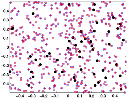
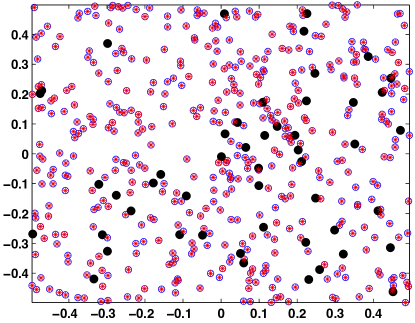
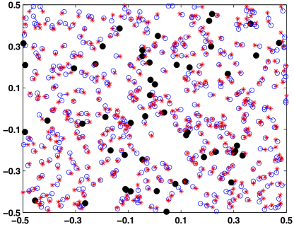
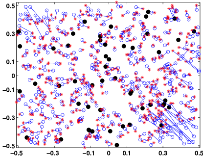
Following [10, 16], we generate the true positions of the sensors and anchors by drawing $|\mathscr{V}|=N+K$ points $\{\boldsymbol{x}_{i}:i\in\mathscr{V}\}$ from the uniform distribution on the unit square $[-0.5,0.5]^{2}$. We take the first $N$ points to be the sensors and the remaining $K$ points to be the anchors. Following [11], we set $K=[N/10]$. The distance graph $\mathscr{G}=(\mathscr{V},\mathscr{E})$ is given by the condition that $(k,l)\in\mathscr{E}$ if and only if $\lVert\boldsymbol{x}_{k}-\boldsymbol{x}_{l}\rVert\leq r$, where $r\in(0,1)$ is the radio range. We also use the noise model from [10, 16] in which the measured distances are given by $d(k,l)=|1+\eta\cdot N(0,1)|\cdot\lVert\boldsymbol{x}_{k}-\boldsymbol{x}_{l}\rVert$ for $(k,l)\in\mathscr{E},$ where $N(0,1)$ is the standard normal distribution and $\eta\in(0,1)$ is the noise level. While other noise models could also be considered, we settled for this noise model to facilitate comparison with the results in [10, 16]. For the same reason, we use the Root-Mean-Squared-Deviation (RMSD) to quantify the localization accuracy which is given by the square root of $(1/N)\sum_{k=1}^{N}\lVert\hat{\boldsymbol{x}}_{k}-\boldsymbol{x}_{k}\rVert^{2}$.

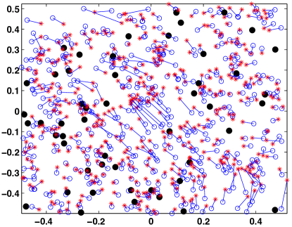
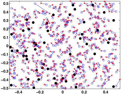
Note that it is possible to register the patches in a globally consistent manner using the anchor-free registration, simply by dropping the equations in (3). Do we get better localization accuracy by incorporating the anchor information into the registration? Exhaustive simulations (not reported here) show that by incorporating anchors into the registration, it is indeed possible to improve the accuracy. Simulations show that if the noise is small and the patches are sufficiently rigid, then the margin of improvement is small. However, under more adversarial settings, the margin can be quite substantial. A particular example is presented in Figure 1. Notice the poor localization in (c) around the top left corner. This is because a couple of patches around this region were poorly localized by SNLSDP, and moreover, the anchors in this region were not considered during the registration. As a consequence, the rigid transform associated with these patches were poorly estimated during the registration. Also, notice that the gradient-based refinement is quite effective in reducing the RMSD in either case. In particular, while the RMSD gap is about $50\%$ after the registration, the gap comes down to about $20\%$ after the refinement.

Table 1: Comparison of the run time and localization accuracy of SNLSR ($t1$ and RMSD1) with [10, 16] ($t2$ and RMSD2) for the unit-square graph. We used SNLSDP [10] for $N<150$, and ESDP [16] for larger problems (see text for further details).

$N$	$r$	$\eta$	$t1$	$t2$	RMSD1	RMSD2
100	0.4	0	8.1 sec	9.1 sec	8.9e-8	2.7e-9
100	0.4	0.3	4.2 sec	8.6 sec	3.1e-2	3.2e-2
150	0.3	0	5.1 sec	38.9 sec	3.8e-8	1.4e-8
150	0.3	0.2	5.6 sec	91.3 sec	2.1e-2	1.9e-2
150	0.2	0.1	6.8 sec	2.1 min	2.5e-2	2.1e-1
500	0.2	0	10.4 sec	2.74 min	3.8e-6	1.2e-7
500	0.2	0.01	21.5 sec	46.1 sec	4.3e-4	8.2e-4
500	0.2	0.1	15.1 sec	37.9 sec	4.3e-3	2.3e-2
1000	0.06	0	32.7 sec	9.35 min	1.9e-2	1.3e-2
1000	0.06	0.01	33.1 sec	5.55 min	3.4e-2	3.2e-2
1000	0.06	0.05	25.7 sec	1.82 min	2.8e-2	1.3e-2
2000	0.04	0	1.84 min	11.35 min	1.3e-2	1.2e-2
2000	0.04	0.005	1.93 min	6.54 min	1.8e-2	1.1e-2
2000	0.04	0.05	1.62 min	7.26 min	1.5e-2	1.1e-2
4000	0.03	0	6.82 min	24.35 min	1.1e-2	1.6e-2
4000	0.03	0.01	6.81 min	22.54 min	1.2e-2	8.2e-3
8000	0.02	0	28.34 min	1 hr 16 min	2.4e-3	4.8e-3

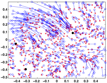
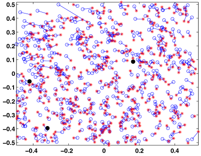
We next compare SNLSR with the SDP-based methods in [10, 16], both in terms of accuracy and scalability. Using the computational resources mentioned earlier, we could solve for at most $N=150$ sensors using SNLSDP [10]. We used ESDP to address larger problems. Simulations suggest that our divide-and-conquer method is significantly faster (often by an order) than these methods. The accuracy of SNLSR is comparable, and occasionally better, than these methods. A visual comparison for a moderate-sized problem is provided in Figure 2. Further comparisons are provided in Table 1. We note that we empirically tuned $\lambda$ in $\phi$ to get the minimum RMSD from SNLSR. For the SNL settings considered here, the optimal $\lambda$ was in the interval $(1,4)$, and the variability of the RMSD within this interval was small (within $10\%$ of the optimal), and even smaller after the refinement.

4 Conclusion

We presented a divide-and-conquer approach for SNL and demonstrated its utility for large-scale problems. In particular, we showed how the non-convex problem of registering the subnetworks can be relaxed and solved efficiently using modern convex programming tools. While the simulation results presented here are far from exhaustive, they nevertheless demonstrate that the idea of localizing patches in parallel and then registering them in a globally consistent fashion can indeed lead to fast and scalable algorithms.

References

- [1] N. Patwari, J. N. Ash, S. Kyperountas, A. O. Hero III, R. L. Moses, and N. S. Correal, “Locating the nodes: cooperative localization in wireless sensor networks,” IEEE Signal Processing Magazine, vol. 22(4), pp. 54-69, 2005.
- [2] M. Tubaishat and S. Madria, “Sensor networks: An overview,” IEEE Potentials, vol. 22(2), pp. 20-23, 2003.
- [3] Y. Yemini, “Some theoretical aspects of location-location problems,” Proc. IEEE Symposium on Foundations of Computer Science, pp. 1-8, 1979.
- [4] T. F. Cox and M. A. A. Cox, Multidimensional Scaling. Monographs on Statistics and Applied Probability 88, Chapman and Hall/CRC, 2001.
- [5] H. Wymeersch, J. Lien, and M. Z. Win, “Cooperative localization in wireless networks,” Proc. IEEE, vol. 97(2), pp. 427-450, 2009.
- [6] R. Olfati-Saber, “Distributed Kalman filtering for sensor networks,” Proc. IEEE Conference on Decision and Control, pp. 5492-5498, 2007.
- [7] F. Chan and H.-C. So, “Accurate distributed range-based positioning algorithm for wireless sensor networks,” IEEE Transactions on Signal Processing, vol. 57(10), pp. 4100-4105, 2009.
- [8] U. A. Khan, S. Kar, and J. F. Moura, “DILAND: An algorithm for distributed sensor localization with noisy distance measurements,” IEEE Transactions on Signal Processing, vol. 58(3), pp. 1940-1947, 2010.
- [9] G. Mao, B. Fidan, and B. Anderson, “Wireless sensor network localization techniques,” Computer Networks, vol. 51(10), pp. 2529-2553, 2007.
- [10] P. Biswas, T.-C. Liang, K.-C. Toh, Y. Ye, and T.-C. Wang, “Semidefinite programming approaches for sensor network localization with noisy distance measurements,” IEEE Transactions on Automation Science and Engineering, vol. 3(4), no. 4, pp. 360-371, 2006.
- [11] P. Tseng, “Second-order cone programming relaxation of sensor network localization,” SIAM Journal on Optimization, vol. 18(1), pp. 156-185, 2007.
- [12] A. Javanmard and A. Montanari, “Localization from incomplete noisy distance measurements,” Proc. IEEE International Symposium on Information Theory, pp. 1584-1588, 2011.
- [13] A. M.-C. So and Y. Ye, “Theory of semidefinite programming for sensor network localization,” Mathematical Programming, vol. 109(2-3), pp. 367-384, 2007.
- [14] K.-C. Toh, M. J. Todd, and R. H. Tutuncu, “SDPT3 – A Matlab software package for semidefinite programming,” version 1.3, Optimization Methods and Software, vol. 11(1-4), pp. 545-581, 1999.
- [15] J. F. Strum, “Using SeDuMi 1.02, A Matlab toolbox for optimization over symmetric cones,” Optimization Methods and Software, vol. 11(1-4), pp. 625-653, 1999.
- [16] Z. Wang, S. Zheng, Y. Ye, and S. Boyd, “Further relaxations of the semidefinite programming approach to sensor network localization,” SIAM Journal on Optimization, vol. 19(2), pp. 655-673, 2008.
- [17] Y. Koren, C. Gotsman, and M. B.-Chen, “PATCHWORK: Efficient localization for sensor networks by distributed global optimization,” Technical Report, 2005.
- [18] L. Zhang, L. Liu, C. Gotsman, and S. Gortler, “An As-Rigid-As-Possible approach to sensor network localization,” ACM Transactions on Sensor Networks, vol. 6(4), pp. 35:1 - 35:21, 2010.
- [19] M. Cucuringu, Y. Lipman, and A. Singer, “Sensor network localization by eigenvector synchronization over the Euclidean group,” ACM Transactions on Sensor Networks, vol. 8(3), pp. 19:1-19:42, 2012.
- [20] J. Shi and J. Malik, “Normalized cuts and image segmentation,” IEEE Transactions on Pattern Analysis and Machine Intelligence, vol. 22(8), pp. 888-905, 2000.
- [21] K. N. Chaudhury, Y. Khoo, and A. Singer, “Global registration of multiple point clouds using semidefinite programming,” SIAM Journal on Optimization, in press, also available at arXiv:1306.5226.
- [22] L. Vandenberghe and S. Boyd, “Semidefinite programming,” SIAM Review, vol. 38(1), pp. 49-95, 1996.
- [23] K. S. Arun, T. S. Huang, and S. D. Blostein, “Least-squares fitting of two 3d point sets,” IEEE Transactions on Pattern Analysis and Machine Intelligence, pp. 698–700, 1987.
- [24] S. Burer and R. D. C. Monteiro, “A nonlinear programming algorithm for solving semidefinite programs via low-rank factorization,” Mathematical Programming, vol. 95(2), 329-357, 2003.