A closed formula for the topological entropy of multimodal maps based on min-max symbols

Abstract Topological entropy is a measure of complex dynamics. In this regard, multimodal maps play an important role when it comes to study low-dimensional chaotic dynamics or explain some features of higher dimensional complex dynamics with conceptually simple models. In the first part of this paper an analytical formula for the topological entropy of twice differentiable multimodal maps is derived, and some basic properties are studied. This expression involves the so-called min-max symbols, which are closely related to the kneading symbols. Furthermore, its proof leads to a numerical algorithm that simplifies a previous one also based on min-max symbols. In the second part of the paper this new algorithm is used to compute the topological entropy of different modal maps. Moreover, it compares favorably to the previous algorithm when computing the topological entropy of the bi- and tri-modal maps considered in the numerical simulations.

1 Introduction

The kneading sequences of a multimodal map $f$ are symbolic sequences that locate the iterates of its critical values up to the precision set by the partition defined by its critical points [1, 2]. Since the $n$th iterate of a critical point of $f$ is a critical value of $f$, it makes sense to attach to the symbols of each kneading sequence of $f$ a label informing about their minimum/maximum (or “critical”) character. The result is a min-max sequence, one per critical point, consisting of min-max symbols. These symbols and sequences were introduced in [3, 4] for unimodal maps, and in [5] for multimodal maps. Thus, min-max sequences generalize kneading sequences in that they additionally provide geometric information about the extrema structure of $f^{n}$ at the critical points for all $n\geq 1$. That this generalization is a good idea, can be justified in several ways, the most direct one being that the computational cost of a min-max symbol is virtually the same as of a kneading symbol for any sufficiently smooth multimodal map. Indeed, the extra piece of information contained in a min-max symbol can be automatically retrieved from a look-up table once the min-max symbol of the previous iterate has been calculated.

Another justification is that min-max sequences allow to construct recursive algorithms to compute the topological entropy [6, 7] of multimodal maps. To this end we assumed in [8, 5] that $f$ is twice differentiable, although numerical simulations with continuous, piecewise linear maps of constant slopes $\pm\left|s\right|$ (and hence, with topological entropy $\log\left|s\right|$ [9]) support the hypothesis that our results hold true under weaker conditions.

In this paper, which is an outgrowth of [5], we derive an analytical formula for the topological entropy of $f$, $h(f)$, that is formally similar to other well-known expressions like [10, 9, 11]

$$h(f) =\lim_{n\rightarrow\infty}\frac{1}{n}\log\ell_{n}$$ (1)

$$=\lim_{n\rightarrow\infty}\frac{1}{n}\log\left|\left\{x\in I:f^{n}(x)=x\right\}\right|$$ (2)

$$=\lim_{n\rightarrow\infty}\frac{1}{n}\log^{+}\text{Var}(f^{n})$$ (3)

$$=\lim_{n\rightarrow\infty}\frac{1}{n}\log^{+}\text{length}(f^{n}),$$ (4)

where (i) $\ell_{n}$ is shorthand for the lap number of $f^{n}$ (i.e., the number of maximal monotonicity segments of $f^{n}$), (ii) $\left|\cdot\right|$ denotes cardinality (i.e., $\left|\left\{x\in I:f^{n}(x)=x\right\}\right|$ is the number of periodic points of period $n$), (iii) Var$(f^{n})$ stands for the variation of $f^{n}$, and (iv) length$(f^{n})$ means the length of the graph of $f^{n}$. The new expression follows from (1) via some geometrical properties for boundary-anchored maps involving min-max symbols. Moreover, its derivation leads to several numerical algorithms to compute $h(f)$. We will only discuss the most simple one, which abridges the algorithm of [5]. Benchmarking of the simplified algorithm with respect to the original one shows that the former sometimes outperforms the latter.

The interest of closed (or analytical) formulas is manifold including, as just mentioned, hypothetical improvements in the speed and precision of already existing algorithms. But, most importantly, analytical formulas usually provide insights into a problem, open alternative ways to prove new properties or attack old problems and, in any case, add techniques to the conceptual and instrumental toolkit of the field. Thus, as compared to the general definition of topological entropy [6, 7], the expressions (1)-(4) are conceptually simpler, besides providing a variety of numerical techniques to compute $h(f)$; see [8, 5] for general algorithms based on the formula (1), and [11, 12, 13, 14, 15, 16, 17, 18] for other mathematical schemes with various degrees of generality.

This paper is organized as follows. In order to make the paper self-contained, we review in Sect. 2 all the basic concepts, especially the concept of min-max sequences, needed for the present sequel. In Sect. 3 we introduce some auxiliary results. In particular, we provide a formal proof of the known fact that the topological entropy does not depend on the boundary conditions. Sect. 4 contains the main result of the paper, namely, a new analytical formula for the topological entropy of multimodal maps (Theorem 1). As way of illustration, this formula is applied in Sect. 5 to a few special cases of multimodal maps whose critical values comply with certain confinement conditions. In Sect. 6 we derive an interesting relation between the value of $h(f)$ and the divergence rate of a logarithmic expression that appears in the analytical formula proved in Theorem 1. A simple algorithm prompted by the proof of Theorem 1 is explained in Sect. 7. This algorithm is put to test in Sect. 8, where the topological entropy of uni-, bi-, and trimodal maps taken from [8, 5] are computed. Its performance is also compared with the algorithm of [5] in those three cases.

2 Min-max sequences

We use the same notation as in [5] throughout.

Let $I$ be a compact interval $[a,b]\subset\mathbb{R}$ and $f:I\rightarrow I$ a piecewise monotone continuous map. Such a map is called $l$-modal if $f$ has precisely $l$ turning points (i.e., points in $(a,b)$ where $f$ has a local extremum). Assume that $f$ has local extrema at $c_{1}<...<c_{l}$ and that $f$ is strictly monotone in each of the $l+1$ intervals

$$I_{1}=[a,c_{1}),I_{2}=(c_{1},c_{2}),...,I_{l}=(c_{l-1},c_{l}),I_{l+1}=(c_{l},b]\text{.}$$

Also as in [5], we assume henceforth that $f(c_{1}$) is a maximum. These maps are said to have positive shape. This implies that $f(c_{2k+1})$, $0\leq k\leq\left\lfloor\frac{l-1}{2}\right\rfloor$, are maxima, whereas $f(c_{2k})$, $1\leq k\leq\left\lfloor\frac{l}{2}\right\rfloor$, are minima. Furthermore, $f$ is strictly increasing on the the intervals $I_{2k+1}$, $0\leq k\leq\left\lfloor\frac{l}{2}\right\rfloor$, and strictly decreasing on the intervals $I_{2k}$, $1\leq k\leq\left\lfloor\frac{l+1}{2}\right\rfloor$.

The itinerary of $x\in I$ under $f$ is a symbolic sequence

$$\mathbf{i}(x)=(i_{0}(x),i_{1}(x),...,i_{n}(x),...)\in\{I_{1},c_{1},I_{2},...,c_{l},I_{l+1}\}^{\mathbb{N}_{0}}$$

($\mathbb{N}_{0}\equiv\{0\}\cup\mathbb{N}$), defined as follows:

$$i_{n}(x)=\left\{\begin{array}[c]{cl}I_{j}&\text{if }f^{n}(x)\in I_{j}\text{ }(1\leq j\leq l+1),\\ c_{k}&\text{if }f^{n}(x)=c_{k}\text{ }(1\leq k\leq l).\end{array}\right.$$

The itineraries of the critical values,

$$\gamma^{i}=(\gamma_{1}^{i},...,\gamma_{n}^{i},...)=\mathbf{i}(f(c_{i})),\;1\leq i\leq l,$$

are called the kneading sequences [2] of $f$.

We turn to the min-max sequences [3, 4, 5, 8] of $f$.

Definition 1. The min-max sequences of an $l$-modal map $f$,

$$\omega^{i}=(\omega_{1}^{i},\omega_{2}^{i},...,\omega_{n}^{i},...),\;1\leq i\leq l,$$

are defined as follows:

$$\omega_{n}^{i}=\left\{\begin{array}[c]{ll}m^{\mathbf{\gamma}_{n}^{i}}&\text{if }f^{n}(c_{i})\text{ is a minimum},\\ M^{\mathbf{\gamma}_{n}^{i}}&\text{if }f^{n}(c_{i})\text{ is a maximum.}\end{array}\right.$$

where $\gamma_{n}^{i}$ are kneading symbols.

Thus, the min-max symbols $\omega_{n}^{i}$ have an exponential-like notation, where the ‘base’ belongs to the alphabet $\{m,M\}$, and the ‘exponent’ is a kneading symbol. Therefore, the extra information of a min-max symbol $\omega^{i}$ as compared to a kneading symbol $\gamma^{i}$ lies in the base.

As in [8, 5] we consider the class $\mathcal{F}_{l}(I)$ of $l$-modal maps $f:I\rightarrow I$ such that

(i) $f\in C^{2}(I)$, and

(ii) $f^{\prime}(x)\neq 0$ for $x\in I_{k}$, $1\leq k\leq l+1$.

That is, a multimodal map $f$ of the interval $I$ belongs to $\mathcal{F}_{l}(I)$ if (i) it is twice differentiable, and (ii) it is strictly monotone except at the turning points. When the interval $I$ is clear from the context or unimportant for the argument, we write just $\mathcal{F}_{l}$.

The next lemma proves our claim in the Introduction that, from the point of view of the computational cost, min-max sequences and kneading sequences are virtually equivalent, at least if $f$ is twice differentiable.

Lemma 1. If $f\in\mathcal{F}_{l}$ has positive shape, then the following ‘transition rules’ hold:

$$\omega_{n}^{i}$$

           (5)

where “even” and “odd” stand for even and odd subindices, respectively, of the critical points $c_{1},...,c_{l}$, and of the intervals $I_{1},...,I_{l}$.

See [5, Lemma 2.2]. Therefore, the kneading symbols of the $f\in\mathcal{F}_{l}$, together with its initial min-max symbols, i.e.

$$\omega_{1}^{i}=\left\{\begin{array}[c]{ll}M^{\gamma_{1}^{i}}&\text{if }i=1,3,...,2\left\lfloor\frac{l+1}{2}\right\rfloor-1,\\ m^{\gamma_{1}^{i}}&\text{if }i=2,4,...,2\left\lfloor\frac{l}{2}\right\rfloor,\end{array}\right.\;$$ (6)

and the transition rules (5) allow to compute the min-max sequences of $f\in\mathcal{F}_{l}$ in a recursive way.

In [8, 5] we used ‘signatures’ instead of kneading symbols in the exponents of $\omega_{n}^{i}$. The signature of a point $x\in[a,b]$ is a vector with $l$ entries, the $i$th entry being $+1$, $0$, or $-1$ according to whether $x>c_{i}$, $x=c_{i}$, or $x<c_{i}$, respectively. It is clear that the signature of $f^{n}(c_{i})$ does the same as $\gamma_{n}^{i}$ when it comes to locate $f^{n}(c_{i})$ in the partition

$$I_{1}\cup\{c_{1}\}\cup I_{2}\cup\{c_{2}\}\cup...,\cup\{c_{l}\}\cup I_{l+1}$$ (7)

of the interval $I=[a,b]$, but in a ‘computer-friendly’ way. For the purposes of this paper though, the computational advantages of signatures will be not needed.

A final ingredient (proper of min-max sequences) is the following. Let the $i$th critical line, $1\leq i\leq l$, be the line $y=c_{i}$ in the Cartesian product $I\times I=\{(x,y):x,y\in I\}$. Min-max symbols divide into bad and good symbols with respect to $i$th critical line. Geometrically, good symbols correspond to local maxima strictly above the line $y=c_{i}$, or to local minima strictly below the line $y=c_{i}$. All other min-max symbols are bad by definition with respect to the $i$th critical line. We use the notation

$$\mathcal{B}^{i}=\{M^{I_{1}},M^{c_{1}},...,M^{I_{i}},M^{c_{i}},m^{c_{i}},m^{I_{i+1}},...,m^{c_{l}},m^{I_{l+1}}\}$$

for the set of bad symbols of $f\in\mathcal{F}_{l}$ with respect to the $i$th critical line. There are $2(l+1)$ bad symbols and $2(l-1)$ good symbols with respect to a given critical line.

Bad symbols appear in all results of [8, 5] concerning the computation of the topological entropy of $f\in\mathcal{F}_{l}$ via min-max symbols. In this sense we may say that bad symbols are the hallmark of this approach.

3 Auxiliary results

In general, Latin indices refer to the critical points and range between $1$ and $l$, while Greek indices refer to the number of iterations, hence they take on arbitrary, nonnegative integer values.

Let $s_{\nu}^{i}$, $1\leq i\leq l$, stand for the number of interior simple zeros of $f^{\nu}(x)-c_{i}$, $\nu\geq 0$, i.e., solutions of $x-c_{i}=0$ ($\nu=0$), or (ii) solutions of $f^{\nu}(x)=c_{i}$, $x\in(a,b)$, with $f^{\mu}(x)\neq c_{i}$ for $0\leq\mu\leq\nu-1$, and $f^{\nu\prime}(x)\not=0$ ($\nu\geq 1$). Geometrically $s_{\nu}^{i}$ is the number of transversal intersections in the Cartesian plane $(x,y)$ of the curve $y=f^{\nu}(x)$ and the straight line $y=c_{i}$, over the interval $(a,b)$. Note that $s_{0}^{i}=1$ for all $i$.

To streamline the notation of the forthcoming math, set

$$s_{\nu}=\sum_{i=1}^{l}s_{\nu}^{i}$$ (8)

for $\nu\geq 0$. In particular,

$$s_{0}=\sum_{i=1}^{l}s_{0}^{i}=\sum_{i=1}^{l}1=l.$$ (9)

According to [5, Eqn. (31)], the lap number of $f^{n}$, $\ell_{n}$, satisfies

$$\ell_{n}=\sum\limits_{\nu=0}^{n-1}s_{\nu}+1.$$ (10)

In particular, $\ell_{1}=l+1$.

Furthermore, define

$$K_{\nu}^{i}=\{(k,\kappa),1\leq k\leq l,1\leq\kappa\leq\nu:\omega_{\kappa}^{k}\in\mathcal{B}^{i}\},$$ (11)

($\nu\geq 1$, $1\leq i\leq l$), that is, $K_{\nu}^{i}$ collects the upper and lower indices $(k,\kappa)$ of the bad symbols with respect to the $i$th critical line in all the initial segments

$$\omega_{1}^{1},\omega_{2}^{1},...,\omega_{\nu}^{1};\;\;\omega_{1}^{2},\omega_{2}^{2},...,\omega_{\nu}^{2};\;\;...;\;\;\omega_{1}^{l},\omega_{2}^{l},...,\omega_{\nu}^{l};$$

of the min-max sequences of $f$. We note for further reference that $K_{\nu-1}^{i}\subset K_{\nu}^{i}$, the set-theoretical difference being

$$K_{\nu}^{i}\backslash K_{\nu-1}^{i}=\{(k,\nu),1\leq k\leq l:\omega_{\nu}^{k}\in\mathcal{B}^{i}\}.$$ (12)

Finally, set

$$S_{\nu}^{i}=2\sum_{(k,\kappa)\in K_{\nu}^{i}}s_{\nu-\kappa}^{k},$$ (13)

where $S_{\nu}^{i}=0$ if $K_{\nu}^{i}=\emptyset$, and analogously to (8),

$$S_{\nu}=\sum_{i=1}^{l}S_{\nu}^{i}.$$ (14)

The algorithm to compute the topological entropy of $f\in\mathcal{F}_{l}$ in [5] rests on the relation [5, Eqn. (32)]

$$s_{\nu}^{i}=1+\sum_{\mu=0}^{\nu-1}s_{\mu}-S_{\nu}^{i}-\alpha_{\nu}^{i}-\beta_{\nu}^{i},$$ (15)

where $\alpha_{\nu}^{i}$,$\beta_{\nu}^{i}$ are binary variables that depend on $f^{\nu}(a)$, $f^{\nu}(b)$, and the $i$th critical line in the way specified in [5, Eqn. (27)]. Let us point out for further reference that all $\alpha_{\nu}^{i}$’s and $\beta_{\nu}^{i}$’s vanish if $f$ is boundary-anchored, i.e., $f\{a,b\}\subset\{a,b\}$. Since we are considering $l$-modal maps with a positive shape, this condition boils down in our case to

$$f(a)=f(b)=a$$

if $l$ is odd, or

$$f(a)=a,\;f(b)=b$$

if $l$ is even.

We are going to show that, as long as the computation of $h(f)$ is concerned, we may assume without loss of generality that $f$ is boundary-anchored. Its proof proceeds by extending $f$ to a selfmap $F$ of a greater interval in such a way that $F$ is boundary-anchored, and $h(f)=h(F)$.

To prove this property, we need the following general facts. Let $g:X\rightarrow X$ be a continuous map of a compact Hausdorff space $X$ into itself. A point $x\in X$ is nonwandering with respect to the map $g$ if for any neighborhood $U$ of $x$ there an $n\geq 1$ (possibly depending on $x$) such that $f^{n}(U)\cap U\neq\emptyset$. Fixed and periodic points are examples of nonwandering points. The closed set of all nonwandering points of $g$ is called its nonwandering set and denoted by $\Omega(g)$. According to [9, Lemma 4.1.5],

$$h(g)=h(\left.g\right|_{\Omega(g)}).$$ (16)

Furthermore, if

$$X=\bigcup\limits_{i=1}^{k}Y_{i}$$

and all $Y_{i}$ are closed and $g$-invariant (i.e., $g(Y_{i})\subset Y_{i})$, then [9, Lemma 4.1.10],

$$h(g)=\max_{1\leq i\leq k}h(\left.g\right|_{Y_{i}}).$$ (17)

Lemma 2. Let $f\in\mathcal{F}_{l}(I)$. Then there exists $F\in\mathcal{F}_{l}(J)$, where $J\supset I$, such that $h(F)=h(f)$ and $F$ is boundary-anchored.

Proof. Set $I=[a,b]$, and $J=[a^{\prime},b^{\prime}]$ with $a^{\prime}\leq a<b\leq b^{\prime}$. If $f(a)=a$, choose $a^{\prime}=a$; if $f(b)=a$ ($l$ odd) or $f(b)=b$ ($l$ even), choose $b^{\prime}=b$. For definiteness, we suppose the most general situation, namely, $a^{\prime}<a$  and $b<b^{\prime}$. Let $F:J\rightarrow J$ be such that (i) $F$ is strictly increasing and twice differentiable on $[a^{\prime},a]$, (ii) $\left.F\right|_{[a,b]}=f$, and (iii) $F$ is strictly decreasing ($l$ odd) or strictly increasing ($l$ even), and twice differentiable on $[b,b^{\prime}]$. Moreover the extension of $f$ to $F$ can be made in such a way that $F$ is twice differentiable at the points $a$ and $b$, hence $F\in\mathcal{F}_{l}(J)$ by construction. As a result, $F$ has the same critical points and values as $f$, and it is boundary-anchored.

Furthermore it is easy to check that $\Omega(F)=\Omega(f)\cup C$, where $C$ is a closed and $F$-invariant set that only contains fixed points. Thus, $h(\left.F\right|_{C})=0$ and, according to (16) and (17),

$$h(F)=h(\left.F\right|_{\Omega(F)})=\max\{h(\left.F\right|_{\Omega(f)}),h(\left.F\right|_{C})\}=h(\left.F\right|_{\Omega(f)})=h(\left.f\right|_{\Omega(f)})=h(f).\;\square$$

The formulation and proof of Lemma 2 was tailored to maps $f\in\mathcal{F}_{l}(I)$ of positive shape. It is plain though that the statement of Lemma 2 holds also true if $f$ is just a continuous selfmap of a closed interval $I$. In this case, $F$ may be taken piecewise linear on $[a^{\prime},a]\cup[b,b^{\prime}]$.

4 A closed formula for the topological entropy of unimodal maps

According to Lemma 2, given $f\in\mathcal{F}_{l}$ we may assume without restriction that it is boundary-anchored when calculating its topological entropy. This being the case, set $\alpha_{\nu}^{i}=\beta_{\nu}^{i}=0$ in (15) for all $\nu\geq 1$ and $i=1,...,l$, i.e.,

$$s_{\nu}^{i}=1+\sum_{\mu=0}^{\nu-1}s_{\mu}-S_{\nu}^{i},$$ (18)

and sum (18) over $i$ from $1$ to $l$ to obtain the relation

$$s_{\nu}=l\left(\sum\limits_{\mu=0}^{\nu-1}s_{\mu}+1\right)-S_{\nu}$$ (19)

between $s_{0}=l,s_{1},...,s_{\nu}$ and $S_{\nu}$, for all $\nu\geq 1$. By (10) this equation can we rewritten as $s_{\nu}=l\ell_{\nu}-S_{\nu}$, hence

$$\ell_{\nu}=\frac{1}{l}(S_{\nu}+s_{\nu}).$$ (20)

Lemma 3. Let $f\in\mathcal{F}_{l}$ be boundary-anchored. Then

$$s_{\nu}=l(l+1)^{\nu}-l\sum_{\delta=1}^{\nu-1}(l+1)^{\nu-\delta-1}S_{\delta}-S_{\nu}$$ (21)

for $\nu\geq 1$, where the summation over $\delta$ is missing for $\nu=1$.

Proof. The proof is by induction. The case $\nu=1$ holds trivially on account of (19) and $s_{0}=l$.

Consider next the case $\nu+1$. By (19) with $\nu+1$ instead of $\nu$,

$$s_{\nu+1} =l+l\sum\limits_{\mu=0}^{\nu}s_{\mu}-S_{\nu+1}=l+ls_{0}+l\sum\limits_{\mu=1}^{\nu}s_{\mu}-S_{\nu+1}$$

$$=l(1+l)+l\sum\limits_{\mu=1}^{\nu}\left(l(l+1)^{\mu}-l\sum_{\delta=1}^{\mu-1}(l+1)^{\mu-\delta-1}S_{\delta}-S_{\mu}\right)-S_{\nu+1}$$ (22)

$$=l(l+1)^{\nu+1}-l\sum\limits_{\mu=1}^{\nu}\left(l\sum_{\delta=1}^{\mu-1}(l+1)^{\mu-\delta-1}S_{\delta}+S_{\mu}\right)-S_{\nu+1}$$ (23)

The induction hypothesis (21) was applied in line (22). The middle term in (23) can be simplified as follows.

$$\sum\limits_{\mu=1}^{\nu}\left(l\sum_{\delta=1}^{\mu-1}(l+1)^{\mu-\delta-1}S_{\delta}+S_{\mu}\right) =l\sum\limits_{\mu=1}^{\nu}\sum_{\delta=1}^{\mu-1}(l+1)^{\mu-\delta-1}S_{\delta}+\sum\limits_{\mu=1}^{\nu}S_{\mu}$$

$$=l\sum_{\delta=1}^{\nu-1}\sum_{k=0}^{\nu-\delta-1}(l+1)^{k}S_{\delta}+\sum\limits_{\mu=1}^{\nu}S_{\mu}$$

$$=\sum_{\delta=1}^{\nu-1}\left((l+1)^{\nu-\delta}-1\right)S_{\delta}+\sum\limits_{\mu=1}^{\nu}S_{\mu}$$

$$=\sum_{\delta=1}^{\nu-1}(l+1)^{\nu-\delta}S_{\delta}+S_{\nu}$$

$$=\sum_{\delta=1}^{\nu}(l+1)^{\nu-\delta}S_{\delta}.$$

Replacement of this into (23) yields

$$s_{\nu+1}=l(l+1)^{\nu+1}-l\sum_{\delta=1}^{\nu}(l+1)^{\nu-\delta}S_{\delta}-S_{\nu+1}.$$ (24)

Comparison of (24) with (21) completes the induction step. $\;\square$

Theorem 1. Let $f\in\mathcal{F}_{l}$. Then

$$h(f)=\log(l+1)-\lim_{\nu\rightarrow\infty}\frac{1}{\nu}\log\frac{1}{1-\sum_{\delta=1}^{\nu-1}\frac{S_{\delta}}{(l+1)^{\delta+1}}},$$ (25)

with $S_{\delta}$ as in (14).

Proof. Without restriction, suppose that $f$ is boundary anchored. From (20) and (21),

$$\ell_{\nu}=\frac{S_{\nu}+s_{\nu}}{l}=(l+1)^{\nu}-\sum_{\delta=1}^{\nu-1}(l+1)^{\nu-\delta-1}S_{\delta}=(l+1)^{\nu}\left(1-\sum_{\delta=1}^{\nu-1}\frac{S_{\delta}}{(l+1)^{\delta+1}}\right).$$ (26)

Use now (1) to derive

$$h(f)=\lim_{\nu\rightarrow\infty}\frac{1}{\nu}\log\ell_{\nu}=\log(l+1)+\lim_{\nu\rightarrow\infty}\frac{1}{\nu}\log\left(1-\sum_{\delta=1}^{\nu-1}\frac{S_{\delta}}{(l+1)^{\delta+1}}\right).\;\square$$

Note that (26) along with (18)-(21) hold true only for boundary-anchored $f\in\mathcal{F}_{l}$. In other words: while the lap numbers $\ell_{\nu}$ depend in general both on the min-max sequences of $f$ (through the sets $K_{\nu}^{i}$ in (13)) and the itineraries of the boundary points of $I$ (through the $\alpha_{\nu}^{i}$’s and $\beta_{\nu}^{i}$’s in (15)), the limit $\lim_{\nu\rightarrow\infty}\frac{1}{\nu}\log\ell_{\nu}=h(f)$ only depends on the min-max sequences.

According to (25), $h(f)\leq\log(l+1)$, a well-known result for multimodal maps. Moreover, (25) expresses the difference $\log(l+1)-h(f)$ for $f\in\mathcal{F}_{l}$ with the help of $(S_{\delta})_{\delta\geq 1}$. The computation of $h(f)$, based on (20), will be addressed in Sect. 7 and 8.

5 Special cases

As way of illustration of the results of Sect. 3, let us consider a few special cases characterized by fulfilling what we call ‘confinement conditions’ for the critical values.

(C1) If $l$ is odd and $f(c_{i})<c_{1}$ for $i=1,...,l$ (so that the graphs of $y=f^{n}(x)$ lie below the first critical line $y=c_{1}$), then (see (5)) $\omega^{\text{odd}}=(M^{I_{1}})^{\infty}$ contains only bad symbols with respect to all critical lines, and $\omega^{\text{even}}=(m^{I_{1}})^{\infty}$ contains only good symbols with respect to all critical lines. Thus,

$$K_{\nu}^{i}=\bigcup\limits_{k=0}^{(l-1)/2}\{(2k+1,1),(2k+1,2),...,(2k+1,\nu)\}.$$

Furthermore, $s_{0}^{i}=1$, and $s_{n}^{i}=0$ for $n\geq 1$, $1\leq i\leq l$, in this case. It follows

$$S_{\nu}=2\sum_{i=1}^{l}\sum_{(k,\kappa)\in K_{\nu}^{i}}s_{\nu-\kappa}^{k}=2\sum_{i=1}^{l}(s_{0}^{1}+s_{0}^{3}+...+s_{0}^{l})=2l\frac{(l+1)}{2}=l(l+1),$$

hence

$$h(f) =\log(l+1)+\lim_{\nu\rightarrow\infty}\frac{1}{\nu}\log\left(1-\sum_{\delta=1}^{\nu-1}\frac{l}{(l+1)^{\delta}}\right)$$

$$=\log(l+1)+\lim_{\nu\rightarrow\infty}\frac{1}{\nu}\log\frac{1}{(l+1)^{\nu-1}}=0.$$

(C2) If $l$ is even and $f(c_{i})<c_{1}$ for all $i=1,...,l$, then the min-max sequences are the same as in case (C1),

$$K_{\nu}^{i}=\bigcup\limits_{k=0}^{l/2-1}\{(2k+1,1),(2k+1,2),...,(2k+1,\nu)\},$$

but this time, due to the branch of $y=f^{n}(x)$ connecting $(c_{l},f^{n}(c_{l}))$ with $(b,b)$, we have $s_{n}^{i}=1$ for $n\geq 0$. It follows

$$S_{\nu}=2\sum_{i=1}^{l}\sum_{(k,\kappa)\in K_{\nu}^{i}}s_{\nu-\kappa}^{k}=2\sum_{i=1}^{l}\sum_{k=0}^{l/2-1}(s_{\nu-1}^{2k+1}+s_{\nu-2}^{2k+1}+...+s_{0}^{2k+1})=2l\tfrac{l}{2}\nu=l^{2}\nu,$$

hence

$$h(f) =\log(l+1)+\lim_{\nu\rightarrow\infty}\frac{1}{\nu}\log\left(1-l^{2}\sum_{\delta=1}^{\nu-1}\frac{\delta}{(l+1)^{\delta+1}}\right)$$

$$=\log(l+1)+\lim_{\nu\rightarrow\infty}\frac{1}{\nu}\log\frac{l\nu+1}{(l+1)^{\nu}}=0.$$

(C3) If $l$ even and $f(c_{i})>c_{l}$ for all $i=1,...,l$, then $\omega^{\text{odd}}=(M^{I_{l+1}})^{\infty}$ and $\omega^{\text{even}}=(m^{I_{l+1}})^{\infty}$. In this case,

$$K_{\nu}^{i}=\bigcup\limits_{k=1}^{l/2}\{(2k,1),(2k,2),...,(2k,\nu)\}.$$

Analogously to case (C2) we also have $s_{n}^{i}=1$ for $n\geq 0$, but now owing to the branch of $y=f^{n}(x)$ connecting $(a,a)$ with $(c_{1},f^{n}(c_{1}))$. Thus

$$S_{\nu}=2\sum_{i=1}^{l}\sum_{(k,\kappa)\in K_{\nu}^{i}}s_{\nu-\kappa}^{k}=2\sum_{i=1}^{l}\sum_{k=1}^{l/2}(s_{\nu-1}^{2k}+s_{\nu-2}^{2k}+...+s_{0}^{2k})=2l\tfrac{l}{2}\nu=l^{2}\nu,$$

as in (C2), hence

$$h(f)=0\text{.}$$

(C4) Finally if $f(c_{\text{odd}})=b$, and $f(c_{\text{even}})=a$, then (see (5))

$$\omega^{\text{odd}}=\left\{\begin{array}[c]{ll}M^{I_{l+1}}(m^{I_{1}})^{\infty}&\text{if }l\text{ is odd,}\\ (M^{I_{l+1}})^{\infty}&\text{if }l\text{ is even,}\end{array}\right.$$

and

$$\omega^{\text{even}}=(m^{I_{1}})^{\infty}\text{.}$$

Thus, in either case both $\omega^{\text{odd}}$ and $\omega^{\text{even}}$ contain only good symbols with respect to all critical lines. It follows that $K_{\nu}^{i}=\emptyset$, hence $S_{\nu}=0$ for all $\nu\geq 1$. We conclude

$$h(f)=\log(l+1)\text{,}$$ (27)

which is the maximum value $h(f)$ can achieve for $f\in\mathcal{F}_{l}$.

6 Convergence

Let us study next the convergence of (25). From (26) it follows

$$1-\sum_{\delta=1}^{\nu-1}\frac{S_{\delta}}{(l+1)^{\delta+1}}=\frac{\ell_{\nu}}{(l+1)^{\nu}}\geq 0$$ (28)

for all $\nu\geq 2$. Hence

$$h(f)=\log(l+1)-\lim_{\nu\rightarrow\infty}\frac{1}{\nu}\log\frac{1}{1-\Sigma_{\nu-1}},$$ (29)

where (see (28))

$$0\leq\Sigma_{\nu}:=\sum_{\delta=1}^{\nu}\frac{S_{\delta}}{(l+1)^{\delta+1}}\leq 1$$ (30)

for $\nu\geq 1$. By definition (30), $\Sigma_{1},..,\Sigma_{\nu},\Sigma_{\nu+1},...$ is a non-negative, non-decreasing sequence of real numbers bounded by 1. Therefore, it converges and

$$\Sigma_{\infty}:=\sum_{\delta=1}^{\infty}\frac{S_{\delta}}{(l+1)^{\delta+1}}=\lim_{\nu\rightarrow\infty}\Sigma_{\nu}\in[0,1].$$

As way of example consider the special cases of Sect. 5. In case (C1)

$$\Sigma_{\infty}=\sum_{\delta=1}^{\infty}\frac{l}{(l+1)^{\delta}}=1,$$

in cases (C2) and (C3)

$$\Sigma_{\infty}=\sum_{\delta=1}^{\infty}\frac{l^{2}\delta}{(l+1)^{\delta+1}}=1,$$

while $\Sigma_{\infty}=0$ in case (C4).

Remember that $A(n)=o(B(n))$ means that $\lim_{n\rightarrow\infty}A(n)/B(n)=0$, and $A(n)\sim B(n)$ means $\lim_{n\rightarrow\infty}A(n)/B(n)=1$.

Theorem 2. Let $f\in\mathcal{F}_{l}$. Then

$$h(f)\in\left\{\begin{array}[c]{ll}\{\log(l+1)\}&\text{if }\log(1-\Sigma_{n})=o(n),\\ [0,\log(l+1))&\text{if }\log(1-\Sigma_{n})\sim-Cn,\end{array}\right.$$ (31)

where $0<C\leq\log(l+1)$.

Proof. According to (29),

$$h(f)=\log(l+1)+\lim_{n\rightarrow\infty}\frac{1}{n}\log(1-\Sigma_{n-1}).$$

Therefore, $h(f)=\log(l+1)$ if $\lim_{n\rightarrow\infty}\frac{1}{n}\log(1-\Sigma_{n-1})=0$, i.e., $\log(1-\Sigma_{n})=o(n)$. Otherwise, $0\leq h(f)<\log(l+1)$ if $\lim_{n\rightarrow\infty}\frac{1}{n}\log(1-\Sigma_{n-1})=-C$ with $0<C\leq\log(l+1)$, i.e., $\log(1-\Sigma_{n})\sim-Cn$.$\;\square$

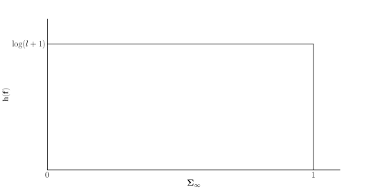
Figure 1: Graph of the inclusion (32).

Theorem 3. Let $f\in\mathcal{F}_{l}$. Then

$$h(f)\in\left\{\begin{array}[c]{ll}\{\log(l+1)\}&\text{if }0\leq\Sigma_{\infty}<1,\\ [0,\log(l+1)]&\text{if }\Sigma_{\infty}=1.\end{array}\right.$$ (32)

Proof. Taking the limit $n\rightarrow\infty$ in (31), one finds that the correspondence $\Sigma_{\infty}\mapsto h(f)$ defines the following inclusion:

$$h(f)\in\left\{\begin{array}[c]{ll}\{\log(l+1)\}&\text{if }0\leq\Sigma_{\infty}<1,\text{ or }\Sigma_{\infty}=1\text{ with }\log(1-\Sigma_{n})=o(n),\\ [0,\log(l+1))&\text{if }\Sigma_{\infty}=1\text{ with }\log(1-\Sigma_{n})\sim-Cn.\end{array}\right.$$ (33)

This proves (32).$\;\square$

Note that in the second case of (33), $h(f)=\log(l+1)-C$ (see the proof of Theorem 2) and $\Sigma_{n}\sim 1-e^{-Cn}$, hence

$$\sum_{\delta=1}^{n}\frac{S_{\delta}}{(l+1)^{\delta+1}}\sim 1-e^{-\left(\log(l+1)-h(f)\right)n}.$$

In other terms, $\Sigma_{n}\nearrow 1$ exponentially fast when $h(f)<\log(l+1)$, the difference $1-\Sigma_{n}$ decreasing as $e^{-\left(\log(l+1)-h(f)\right)n}$.

Figure 1 depicts the inclusion (32): If $h(f)=\log(l+1)$ then $0\leq\Sigma_{\infty}\leq 1$; if $\Sigma_{\infty}=1$ then $0\leq h(f)\leq\log(l+1)$.

7 A simplified algorithm for the topological entropy

When it comes to calculate numerically $h(f)=\lim_{\nu\rightarrow\infty}\frac{1}{\nu}\log\ell_{\nu}$ via Eqn. (26), used in the proof of Theorem 1, the intermediate expression

$$h(f)=\lim_{\nu\rightarrow\infty}\frac{1}{\nu}\log\frac{S_{\nu}+s_{\nu}}{l}$$ (34)

is more efficient and numerically stable than the final expression

$$h(f)=\log(l+1)+\lim_{\nu\rightarrow\infty}\frac{1}{\nu}\log\left(1-\sum_{\delta=1}^{\nu-1}\frac{S_{\delta}}{(l+1)^{\delta+1}}\right).$$ (35)

The computation of $S_{\nu}^{i}$, $1\leq i\leq l$, requires $s_{0}^{i}=1,s_{1}^{i},...,s_{\nu-1}^{i}$, see (13), while the computation of $s_{\nu}^{i}$, $1\leq i\leq l$, requires $s_{0}^{i},s_{1}^{i},...,s_{\nu-1}^{i}$, and $S_{\nu}^{i}$, see (18).

We summarize the algorithm resulting from (34) in the following scheme (“$A\longrightarrow B$” stands for “$B$ is computed by means of $A$”).

(A1)

Parameters: $l\geq 1$ (number of critical points), $\varepsilon>0$ (dynamic halt criterion), and $n_{\max}\geq 2$ (maximum number of loops).

(A2)

Initialization: $s_{0}^{i}=1$, and $K_{1}^{i}=\{k,1\leq k\leq l:\omega_{1}^{k}\in\mathcal{B}^{i}\}$ ($1\leq i\leq l$).

(A3)

First iteration: For $1\leq i\leq l$,

$$\begin{array}[c]{rcll}s_{0}^{i},K_{1}^{i}&\longrightarrow&S_{1}^{i},S_{1}&\text{(use (\ref{notation0}), (\ref{notation}))}\\ s_{0}^{i},S_{1}^{i}&\longrightarrow&s_{1}^{i},s_{1}&\text{(use (\ref{sinu}), (\ref{account}))}\end{array}$$

(A4)

Computation loop. For $1\leq i\leq l$ and $\nu\geq 2$ keep calculating $K_{\nu}^{i}$, $S_{\nu}^{i}$, and $s_{\nu}^{i}$ according to the recursions

$$\begin{array}[c]{rcll}K_{\nu-1}^{i}&\longrightarrow&K_{\nu}^{i}&\text{(use (\ref{Kni2}), (\ref{transition}))}\\ s_{0}^{i},s_{1}^{i},...,s_{\nu-1}^{i},K_{\nu}^{i}&\longrightarrow&S_{\nu}^{i},S_{\nu}&\text{(use (\ref{notation0}), (\ref{notation}))}\\ s_{0}^{i},s_{1}^{i},...,s_{\nu-1}^{i},S_{\nu}^{i}&\longrightarrow&s_{\nu}^{i},s_{\nu}&\text{(use (\ref{sinu}), (\ref{account}))}\end{array}$$ (36)

until (i)

$$\left|\frac{1}{\nu}\log\frac{S_{\nu}+s_{\nu}}{l}-\frac{1}{\nu-1}\log\frac{S_{\nu-1}+s_{\nu-1}}{l}\right|\leq\varepsilon,$$ (37)

or, else, (ii) $\nu=n_{\max}+1$.

(A5)

Output. In case (i) output

$$h(f)=\frac{1}{\nu}\log\frac{S_{\nu}+s_{\nu}}{l}.$$ (38)

In case (ii) output “Algorithm failed”.

The algorithm (A1)-(A5) simplifies the original algorithm [5], which is based on the exact value of the lap number $\ell_{\nu}$. This entails that the new algorithm needs more loops to output $h(f)$ with the same parameter $\varepsilon$ in the halt criterion (37), although this does not necessarily mean that the overall execution time will be longer since now less computations are required. In fact, we will find both situations in the numerical simulations below.

Two final remarks:

R1.

The parameter $\varepsilon$ does not bound the error $\left|h(f)-\frac{1}{\nu}\log\frac{S_{\nu}+s_{\nu}}{l}\right|$ but the difference between two consecutive estimations, see (37). The number of exact decimal positions of $h(f)$ can be found out by taking different $\varepsilon$’s , as we will see in the next section. Equivalently, one can control how successive decimal positions of $\frac{1}{\nu}\log\frac{S_{\nu}+s_{\nu}}{l}$ stabilize with growing $\nu$. Moreover, the smaller $h(f)$, the smaller $\varepsilon$ has to be chosen to achieve a given approximation precision.

R2.

According to [9, Thm. 4.2.4], $\frac{1}{\nu}\log\ell_{\nu}\geq h(f)$ for any $\nu$. We may expect therefore that the numerical approximations (38) converge from above to the true value of the topological entropy with ever more iterations, in spite of the relation $\ell_{\nu}=\frac{1}{l}(S_{\nu}+s_{\nu})$ holding in general for boundary-anchored maps only.

8 Numerical simulations

In this section we calculate the topological entropy of families of uni-, bi-, and trimodal maps taken from [8] and [5]; none of these maps is boundary-anchored. The purpose of our choice is to compare the performance of the simplified algorithm with the original one. To this end, a code for arbitrary $l$ was written with PYTHON, and run on an Intel(R) Core(TM)2 Duo CPU. All logarithms were taken to base $e$, i.e., the values of the topological entropy in this section are given in nats per iteration. The numerical results will be given with six decimal positions for brevity.

8.1 Simulation with 1-modal maps

Let $\alpha>0$, $-1<\beta\leq 0$, and $f_{\alpha,\beta}:[-(1+\beta),(1+\beta)]\rightarrow[-(1+\beta),(1+\beta)]$ be defined as [8, Eqn. (29)]

$$f_{\alpha,\beta}(x)=e^{-\alpha^{2}x^{2}}+\beta.$$

These maps have the peculiarity of showing direct and reverse period-doubling bifurcations when the parameters are monotonically changed [8, Fig. 3(a)].

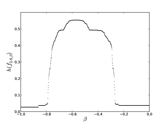
Fig. 2 shows the plot of $h(f_{2.8,\beta})$ vs $\beta$ calculated with the algorithm of Sect. 7. Here $\varepsilon=10^{-4}$ and the parameter $\beta$ was increased in steps of $\Delta\beta=0.001$ from $\beta=-0.999$ to $\beta=0$. Upon comparing Fig. 2 with Fig. 3(b) of [8], we see that both plots coincide visually, except for the two vanishing entropy tails. We conclude that $\varepsilon=10^{-4}$ is not small enough to obtain reliable estimations of the topological entropy for vanishing values of $h(f_{2.8,\beta})$. This fact can also be ascertained numerically by taking different values of $\varepsilon$, as we do in the table below.

Figure 2: Plot of $h(f_{2.8,\beta})$ vs $\beta$, $-1<\beta\leq 0$ ($\varepsilon=10^{-4},\Delta\beta=0.001$).

In order to compare the convergence speed and execution time of the original ([8, 5]) and the simplified algorithm, we have computed $h(f_{2.8,-0.5})$ with both algorithms for different $\varepsilon$’s. The number of loops $n$ needed to achieve the halt condition $\varepsilon=10^{-d}$, $4\leq d\leq 7$, and the execution time $t$ (in seconds) are listed in Table 1. The columns $h_{orig}$, $n_{orig}$, and $t_{orig}$ were obtained with the original algorithm, while the columns $h_{simp}$, $n_{simp}$, and $t_{simp}$ were obtained with the simplified one. For all choices of $\varepsilon$, $t_{orig}<t_{simp}$. Furthermore, we conclude from Table 1 that $h(f)=0.524...$ using the original algorithm, while $h(f)=0.52...$ using the simplified one and the same set of $\varepsilon$’s.

	$h_{orig}$	$n_{orig}$	$t_{orig}$	$h_{simp}$	$n_{simp}$	$t_{simp}$
$\varepsilon=10^{-4}$	0.531968	81	0.024452	0.534106	101	0.023519
$\varepsilon=10^{-5}$	0.526645	253	0.200861	0.527305	318	0.217069
$\varepsilon=10^{-6}$	0.524935	797	1.87643	0.525142	1004	2.126501
$\varepsilon=10^{-7}$	0.524391	2519	18.404195	0.524456	3174	21.399207

Table 1: Comparison of performances when computing $h(f_{2.8,-0.5})$.

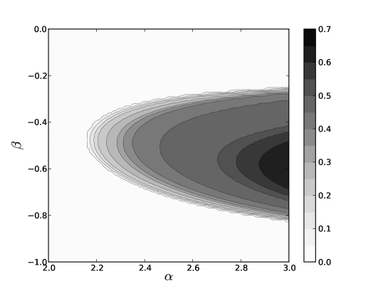
Fig. 3 depicts the values of $h(f_{\alpha,\beta})$ for $2\leq\alpha\leq 3$, $-1<\beta\leq 0$, $\varepsilon=10^{-4}$, and $\Delta\alpha,\Delta\beta=0.01$.

Figure 3: Level sets of $h(f_{\alpha,\beta})$ vs $\alpha,\beta$, $2\leq\alpha\leq 3$, and $-1<\beta\leq 0$ ($\varepsilon=10^{-4},\Delta\alpha=\Delta\beta=0.01$).

8.2 Simulation with 2-modal maps

Let $0\leq v_{2}<v_{1}\leq 1$ and $f_{v_{1},v_{2}}:[0,1]\rightarrow[0,1]$ be defined as [5, Sect. 8.1]

$$f_{v_{1},v_{2}}(x)=(v_{1}-v_{2})(16x^{3}-24x^{2}+9x)+v_{2},$$

These maps have convenient properties for numerical simulations as they share the same fixed critical points,

$$c_{1}=1/4,\;c_{2}=3/4,$$

the critical values are precisely the parameters,

$$f_{v_{1},v_{2}}(1/4)=v_{1},\;f_{v_{1},v_{2}}(3/4)=v_{2},$$

and the values of $f$ at the endpoints are explicitly given by the parameters as follows:

$$f_{v_{1},v_{2}}(0)=v_{2},\;f_{v_{1},v_{2}}(1)=v_{1}.$$

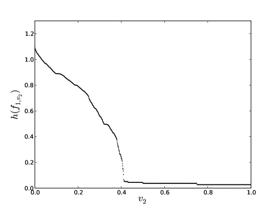
Fig. 4 shows the plot of $h(f_{1,v_{2}})$ vs $v_{2}$, $0\leq v_{2}<1$, computed with the new algorithm, $\varepsilon=10^{-4}$, and $\Delta v_{2}=0.001$. Again, this plot coincides visually with the same plot computed with the old algorithm [5, Fig. 4] except for the vanishing entropy tail, which indicates that $\varepsilon=10^{-4}$ is too large a value for obtaining accurate estimates in that parametric region.

Figure 4: Plot of $h(f_{1,v_{2}})$ vs $v_{2}$, $0\leq v_{2}\leq 1$ ($\varepsilon=10^{-4},\Delta v_{2}=0.001$).

Table 2 displays the performance of the new algorithm as compared to the old one when computing $h(f_{0.9,0.1})$. This time $t_{orig}>t_{simp}$ for $\varepsilon=10^{-d}$, $4\leq d\leq 7$ (as in Table 1). Furthermore, we obtain two exact decimal positions of the topological entropy, $h(f_{0.9,0.1})=0.41...$, with both algorithms and the $\varepsilon$’s considered.

	$h_{orig}$	$n_{orig}$	$t_{orig}$	$h_{simp}$	$n_{simp}$	$t_{simp}$
$\varepsilon=10^{-4}$	0.432246	162	0.228102	0.434175	182	0.202511
$\varepsilon=10^{-5}$	0.421287	511	2.1436	0.42191	573	1.973616
$\varepsilon=10^{-6}$	0.417812	1613	20.918574	0.418008	1810	19.738665
$\varepsilon=10^{-7}$	0.41671	5099	207.190258	0.416772	5721	182.951993

Table 2: Comparison of performances when computing $h(f_{0.9,0.1})$.

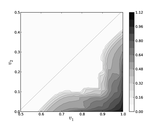
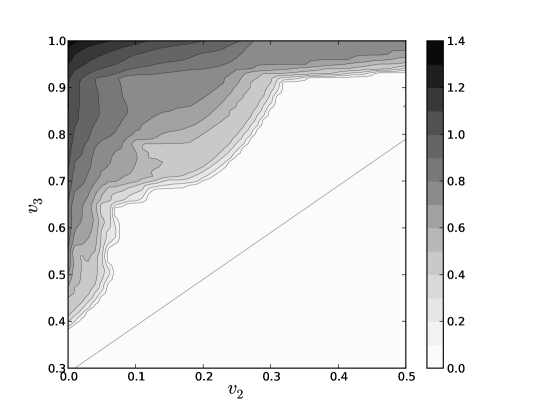
Fig. 5 depicts the values of $h(f_{v_{1},v_{2}})$ for $0\leq v_{2}\leq v_{1}-0.5$, $\varepsilon=10^{-4}$, and $\Delta v_{1},\Delta v_{2}=0.01$.

Figure 5: Level sets of $h(f_{v_{1},v_{2}})$ vs $v_{1},v_{2}$, $0\leq v_{2}\leq v_{1}-0.5$ ($\varepsilon=10^{-4},\Delta v_{1}=\Delta v_{2}=0.01$).

8.3 Simulation with 3-modal maps

Consider next the $3$-modal maps $f_{v_{2},v_{3}}:[0,1]\rightarrow[0,1]$ defined by the quartic polynomials [5, Sect. 8.2]

$$f_{v_{2},v_{3}}(x) =\frac{4\left[\left(2\sqrt{2}-1\right)v_{2}-2v_{3}\right]x}{2(2\sqrt{2}+1)v_{3}-7v_{2}}\left[4\left(1+2\sqrt{2}\right)(x-1)(1-2x)^{2}v_{3}\right.$$

$$+\left.\left(-56x^{3}+20\left(4+\sqrt{2}\right)x^{2}-\left(37+18\sqrt{2}\right)x+3\sqrt{2}+5\right)v_{2}\right],$$

where $0\leq v_{2}<v_{3}\leq 1$. The critical points of $f_{v_{2},v_{3}}$ are

$$c_{1}=\frac{-\sqrt{2}\text{$v_{2}$}-4\text{$v_{2}$}+12\sqrt{2}\text{$v_{3}$}-8\text{$v_{3}$}}{8\left(-7\text{$v_{2}$}+4\sqrt{2}\text{$v_{3}$}+2\text{$v_{3}$}\right)},\quad c_{2}=1/2,\quad c_{3}=\frac{1}{4}(2+\sqrt{2}).$$

Moreover this family verifies $f_{v_{2},v_{3}}(0)=0$, $f_{v_{2},v_{3}}(c_{2})=v_{2}$, $f(c_{3})=v_{3}$, and

$$f_{v_{2},v_{3}}(1)=\frac{4\left(5\sqrt{2}-8\right)\text{$v_{2}$}\left(\left(2\sqrt{2}-1\right)\text{$v_{2}$}-2\text{$v_{3}$}\right)}{-7\text{$v_{2}$}+4\sqrt{2}\text{$v_{3}$}+2\text{$v_{3}$}}.$$

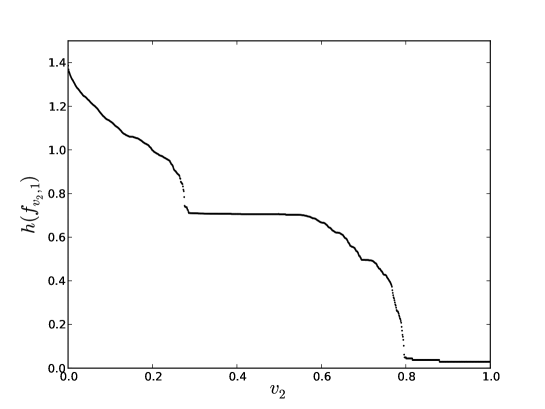
Fig. 6 shows the plot of $h(f_{v_{2},1})$ vs $v_{2}$, $0\leq v_{2}<1$, computed with the new algorithm, $\varepsilon=10^{-4}$, and $\Delta v_{2}=0.001$. Once more, this plot coincides visually with the same plot computed with the old algorithm [5, Fig. 7 (left)] except for the vanishing entropy tail, which again indicates that $\varepsilon=10^{-4}$ is too large a value for obtaining accurate estimates in that parametric region.

Figure 6: Plot of $h(f_{v_{2},1})$ vs $v_{2}$, $0\leq v_{2}<1$ ($\varepsilon=10^{-4},\Delta v_{2}=0.001$).

Table 3 displays the performance of the new algorithm as compared to the old one when computing $h(f_{0.7,1})$. Also this time $t_{orig}>t_{simp}$ for $\varepsilon=10^{-d}$, $4\leq d\leq 7$ (as in Table 1 and 2). Furthermore, we obtain two exact decimal positions of the topological entropy, $h(f_{0.7,1})=0.48...$, with both algorithms and the $\varepsilon$’s considered.

	$h_{orig}$	$n_{orig}$	$t_{orig}$	$h_{simp}$	$n_{simp}$	$t_{simp}$
$\varepsilon=10^{-4}$	0.494586	135	0.304254	0.49579	147	0.251014
$\varepsilon=10^{-5}$	0.48545	426	2.920753	0.48583	464	2.465768
$\varepsilon=10^{-6}$	0.482554	1345	28.715971	0.482675	1465	24.594864
$\varepsilon=10^{-7}$	0.481637	4250	290.400729	0.481675	4630	256.136796

Table 3: Comparison of performances when computing $h(f_{0.7,1})$.

Finally, Fig. 7 depicts the values of $h(f_{v_{2},v_{3}})$ for $v_{2}+0.3\leq v_{3}\leq 1$, $\varepsilon=10^{-4}$, and $\Delta v_{2},\Delta v_{3}=0.01$.

Figure 7: Level sets of $h(f_{v_{2},v_{3}})$ vs $v_{2},v_{3}$, $v_{2}+0.3\leq v_{3}\leq 1$ ($\varepsilon=10^{-4},\Delta v_{1}=\Delta v_{2}=0.01$).

A concluding observation. As anticipated in the remark R2 of Sect. 7 and illustrated in the Tables 1-3, the values of $h_{simp}$ converge from above with ever more computation loops (or smaller values of the parameter $\varepsilon$). This property follows for $h_{orig}$ from [9, Thm. 4.2.4].

9 Conclusion

We provided in Thm. 1, Eqn. (25), an analytical formula to calculate the topological entropy of a multimodal map $f$. The peculiarity of Eqn. (25), as compared to similar formulas (see (1)-(4)), is that it involves the min-max sequences of $f$. Min-max sequences generalize kneading sequences in that they contain additional, geometric information (about the extrema structure of $f^{n}$, $n\geq 1$) but with no computational penalty. We also discussed in Sect. 6 the relationship between the value of $h(f)$ and the divergence rate of $\log(1-\Sigma_{n})$ (or convergence rate of $\Sigma_{n}$ to $1$). It turns out that both are related in the way stated in Thms. 2 and 3. A practical offshoot of Thm. 1 is the algorithm of Sect. 7 to compute $h(f)$. This algorithm is a simplified version of a previous one derived in [5]. The performances of both algorithms were compared in Sect. 8 using uni-, bi-, and trimodal maps. In view of the results summarized in tables 1 to 3, the original algorithm seems to perform better in the unimodal case, while the opposite occurs in the bimodal and trimodal cases.

Acknowledgements. We thank very much the referees of this paper for their constructive criticism. We are also grateful to José S. Cánovas and María Muñoz Guillermo (Universidad Politécnica de Cartagena, Spain), and Víctor Jiménez (Universidad de Murcia, Spain) for clarifying discussions. This work was financially supported by the Spanish Ministerio de Economía y Competitividad, grant MTM2012-31698.

References

• [1] J. Milnor, W. Thurston, On iterated maps of the interval, in: Alexander, J.C. (Ed.), Dynamical Systems, Lectures Notes in Mathematics 1342, Springer, 1988, pp. 465-563.
• [2] W. de Melo, S. van Strien, One-Dimensional Dynamics, Springer, New York, 1993.
• [3] J. Dias de Deus, R. Dilão, J. Taborda Duarte, Topological entropy and approaches to chaos in dynamics of the interval, Phys. Lett. 90A (1982) 1-4.
• [4] R. Dilão, Maps of the interval, symbolic dynamics, topological entropy and periodic behavior (in Portuguese), Ph.D. Thesis, Instituto Superior Técnico, Lisbon (1985).
• [5] J.M. Amigó, R. Dilão, A. Giménez, Computing the Topological Entropy of Multimodal Maps via Min-Max Sequences, Entropy 14 (2012) 742-768.
• [6] R. Adler, A. Konheim, M. McAndrew, Topological entropy, Trans. Amer. Mat. Soc. 114 (1965) 309-319.
• [7] P. Walters, An Introduction to Ergodic Theory, Springer Verlag, New York, 2000.
• [8] R. Dilão, J.M. Amigó, Computing the topological entropy of unimodal maps, International Journal of Bifurcations and Chaos 22 (2012) 1250152.
• [9] L. Alsedà, J. Llibre, M. Misiurewicz, Combinatorial Dynamics and Entropy in Dimension One, World Scientific, Singapore, 2000.
• [10] M. Misiurewicz, W. Szlenk, Entropy of piecewise monotone mappings, Studia Math. 67 (1980) 45-63.
• [11] N.J. Balmforth, E.A. Spiegel, C. Tresser, Topological Entropy of One-Dimensional Maps: Approximations and Bounds, Phys. Rev. Lett. 72 (1994) 80-83.
• [12] S.L. Baldwin, E.E. Slaminka, Calculating topological entropy, J. Stat. Phys. 89 (1997) 1017-1033.
• [13] L. Block, J. Keesling, S. Li, K. Peterson, An improved algorithm for computing topological entropy, J. Stat. Phys. 55 (1989) 929-939.
• [14] L. Block, J. Keesling, Computing the topological entropy of maps pf the interval with three monotone pieces, J. Stat. Phys. 66 (1991) 755-774.
• [15] P. Collet, J.P. Crutchfield, J.P. Eckmann, Computing the topological entropy of maps, Comm. Math. Phys. 88 (1983) 257–262.
• [16] G. Froyland, R. Murray, D. Terhesiu, Efficient computation of topological entropy, pressure, conformal measures, and equilibrium states in one dimension, Phys. Rev. E 76 (2007) 036702.
• [17] P. Góra, A. Boyarsky, Computing the topological entropy of general one-dimensional maps, Trans. Amer. Math. Soc. 323 (1991) 39–49.
• [18] T. Steinberger, Computing the topological entropy for piecewise monotonic maps on the interval, J. Stat. Phys. 95 (1999) 287–303.