Self-consistent energy approximation for orbital-free density-functional theory

Abstract

Employing a local formula for the electron-electron interaction energy, we derive a self-consistent approximation for the total energy of a general $N$-electron system. Our scheme works as a local variant of the Thomas-Fermi approximation and yields the total energy and density as a function of the external potential, the number of electrons, and the chemical potential determined upon normalization. Our tests for Hooke’s atoms, jellium, and model atoms up to $\sim 1000$ electrons show that reasonable total energies can be obtained with almost a negligible computational cost. The results are also consistent in the important large-$N$ limit.

I Introduction

Orbital-free density-functional theory (OF-DFT) is a computationally appealing method to deal with large systems beyond the reach of conventional DFT. At present, OF-DFT methods can handle systems up to a million atoms HungCarter . As the name suggests, OF-DFT is free from the use of the single-particle orbitals needed in the calculation of the kinetic energy in the Kohn-Sham formulation. Thus, the only explicitly required variable is the electron density $\rho({\bf r})$. The earliest OF-DFT method dates back to the Thomas-Fermi (TF) theory employing the exact result of the homogeneous electron gas for the kinetic energy, and the Hartree approximation for the e-e interaction. In fact, most orbital-free schemes can be regarded as modifications or improvements to the TF method of-reviews .

Some of the present authors have previously reconstructed a local total-energy approximation of Parr parr into a two-dimensional (2D) form orb to calculate the energies of large quantum-dot systems. Recently, this 2D approximation was transformed into a self-consistent OF functional that is able to produce reasonable estimations for the total energy of various large 2D systems at a negligible computational cost new . In this respect, it is natural to ask whether the original construction of Parr parr can be made both self-consistent and “instantaneous”, and whether it can provide reasonable results for three-dimensional (3D) structures. The answers to these questions turn out to be positive: here a self-consistent, orbital-free functional is constructed in such a way that it yields relatively good results for a variety of systems including Hooke’s atoms, jellium, and model atoms up to the large-$N$ limit. The functional is also flexible regarding further non-empirical modifications.

II Orbital-free functional

II.1 Parr approximation for the interaction energy

In order to improve the TF theory, an orbital-free local approximation for the electron-electron interaction energy was proposed by Parr parr . Here we summarize the main steps in the derivation. The electron-electron interaction energy can be expressed (in Hartree atomic units) as

$$W=\int d{\bf r}_{1}\int\frac{\rho_{2}({\bf r}_{1},{\bf r}_{2})}{|{\bf r}_{1}-{\bf r}_{2}|}\,d{\bf r}_{2}$$ (1)

where

$$\rho_{2}({\bf r}_{1},{\bf r}_{2}) = \frac{N(N-1)}{2}\sum_{\sigma_{1},\sigma_{2}}\int{d3}...\int dN$$ (2)

$$\times |\Psi({\bf r}_{1}\sigma_{1},{\bf r}_{2}\sigma_{2},3,...,N)|^{2}.$$

is the pair density. Here, $\Psi(1,2,...,N)$ stands for the ground-state many-body wave function and $\int dN$ denotes the spatial integration and spin summation over the $N$th spatial spin coordinate $({\bf r}_{N}\sigma_{N})$. The pair density satisfies the normalization condition

$$\frac{N(N-1)}{2}=\int d{\bf r}_{1}\int\rho_{2}({\bf r}_{1},{\bf r}_{2})d{\bf r}_{2}.$$ (3)

Here, $\rho_{2}$ can be interpreted as the distribution of the electronic pairs orb . We may derive a local-density approximation for the interaction energy $W$ defined in Eq. (1). Firstly, we introduce the interparticle coordinates as

$${\bf r}=({\bf r}_{1}+{\bf r}_{2})/2,\quad{\bf s}={\bf r}_{1}-{\bf r}_{2},$$ (4)

so that $\rho_{2}({\bf r}_{1},{\bf r}_{2})=\rho_{2}({\bf r}+{\bf s}/2,{\bf r}-{\bf s}/2)$. Equation (1) can be rewritten as

$$W=4\pi\int d{\bf r}\int\rho_{2}({\bf r},{\bf s})sds,$$ (5)

where

$$\rho_{2}({\bf r},{\bf s})=\frac{1}{4\pi}\int\rho_{2}\left({\bf r}+\frac{{\bf s}}{2},{\bf r}-\frac{s}{2}\right)\,d\Omega_{s}$$ (6)

is the spherical average of $\rho_{2}({\bf r},{\bf s})$. We can take a Taylor expansion of this term, leading to

$$\rho_{2}({\bf r},s)\approx\rho_{2}({\bf r},{\bf r})\left[1-\frac{s^{2}}{2\beta_{2}({\bf r})}+...\right],$$ (7)

and assume a Gaussian approximation to be valid, i.e.,

$$\rho_{2}({\bf r},s)\approx\rho_{2}({\bf r},{\bf r})\exp\left[-\frac{s^{2}}{2\beta_{2}({\bf r})}\right],$$ (8)

where $\beta_{2}({\bf r})$ is a function of ${\bf r}$ determined below. Substituting Eq. (8) to Eq. (5) leads to

$$W=4\pi\int\rho_{2}({\bf r},{\bf r})\beta_{2}({\bf r})d{\bf r},$$ (9)

and similarly, substituting Eq. (8) to Eq. (3) yields

$$N(N-1)=2(2\pi)^{3/2}\int\rho_{2}({\bf r},{\bf r})\beta_{2}({\bf r})d{\bf r}.$$ (10)

We assume that $\rho_{2}({\bf r},{\bf r})$ and $\beta_{2}({\bf r})$ are both local functions of the electron density. So we may write

$$\rho_{2}({\bf r},{\bf r})=\rho_{2}(\rho({\bf r}))$$ (11)

and

$$\beta_{2}({\bf r})=\beta_{2}(\rho({\bf r})).$$ (12)

The dependencies on the electron densities can be worked out by a dimensional argument. Under uniform scaling of coordinates, ${\bf r}\rightarrow\lambda{\bf r}$ (with $0<\lambda<\infty$), the norm-preserving many-electron wave function is given by

$$\Psi_{\lambda}({\bf r}_{1},...,{\bf r}_{N})=\lambda^{N}\Psi(\lambda{\bf r}_{1},...,\lambda{\bf r}_{N}).$$ (13)

The other quantities scale as

$$\rho_{2,\lambda}({\bf r}_{1},{\bf r}_{2})=\lambda^{4}\rho_{2}(\lambda{\bf r}_{1},\lambda{\bf r}_{2}),$$ (14)

$$\rho_{\lambda}({\bf r})=\lambda^{2}\rho(\lambda{\bf r})$$ (15)

and

$$W[\Psi_{\lambda}]=\lambda W[\Psi].$$ (16)

Using a dimensional argument on Eq. (9) and Eq. (10) leads further to

$$\rho_{2}({\bf r},{\bf r})\beta_{2}({\bf r})=A_{1}\rho^{4/3}({\bf r}),\quad\rho_{2}({\bf r},{\bf r})\beta_{2}^{3/2}(r)=A_{2}\rho({\bf r})$$ (17)

or

$$\rho_{2}({\bf r},{\bf r})=A_{3}\rho^{2}({\bf r}),\quad\beta_{2}({\bf r})=A_{4}\rho^{-2/3}({\bf r}),$$ (18)

where $A_{1}$, $A_{2}$, $A_{3}$ and $A_{4}$ are constants. By considering the Hartree-Fock (HF) case, we can obtain $A_{3}$ from a known relation

$$\rho_{2}({\bf r},{\bf r})=\frac{1}{4}\rho({\bf r})\rho({\bf r}),$$ (19)

so that $A_{3}=1/4$. The other constant $A_{4}$ can be determined by imposing the normalization condition in Eq. (10), leading to

$$A_{4}=\frac{(N-1)^{2/3}}{2^{1/3}\pi}.$$ (20)

Finally, we have all information to express the approximation for the electron-electron interaction energy, which results in a simple form

$$W[\rho] = \frac{(N-1)^{2/3}}{2^{1/3}}\int\rho^{4/3}({\bf r})\,d{\bf r}$$ (21)

$$\approx 0.7937\,(N-1)^{2/3}\int\rho^{4/3}({\bf r})\,d{\bf r}$$

II.2 Bounds for the interaction energy

Gadre et al. gadre have derived an upper bound for the Hartree energy

$$E_{H} = \frac{1}{2}\int d{\bf r}\int d{\bf r}^{\prime}\frac{\rho({\bf r})\rho({\bf r}^{\prime})}{|{\bf r}-{\bf r}^{\prime}|}$$ (22)

$$\leq E_{H}^{\rm max}=1.0918\,N^{2/3}\int\rho^{4/3}({\bf r})\,d{\bf r}.$$

It is interesting to notice the similarity of this bound to the expression for $W$ in Eq. (21). First, we point out that a condition $W\leq E_{H}$ always applies, since $W$ is expected to account for the full interaction energy including both the Hartree energy and the indirect one (cf. exchange and correlation energy in DFT) that is negative by definition. Therefore, we may write an upper bound for $W$ as

$$W[\rho]\leq 1.0918\,N^{2/3}\int\rho^{4/3}({\bf r})\,d{\bf r}.$$ (23)

We immediately notice that Eq. (21) satisfies this bound by a very large margin. Therefore, it is natural to ask how tight the bound is. We examine the tightness by considering a simple test case: a spherical $N$-electron system with radius $R$ and a constant density. The relevance of this model system in terms of the Lieb-Oxford bound lo ; lo2 is analyzed in Ref. paola . The radial density is given simply by $\rho(r)=3N/(4\pi R^{3})$ at $r\leq R$ and zero otherwise. The Hartree energy becomes $E_{H}=3N^{2}/(5R)=0.6\,N^{2}/R$. On the other hand, the Hartree bound condition in this system becomes $E_{H}^{\rm max}\approx 0.6773\,N^{2}/R$. Therefore, the bound is satisfied, but by a relatively slight margin.

This above result suggests that if we require our functional for the interaction energy to apply in the large-$N$ limit, where $N-1\approx N$ and $W\rightarrow E_{H}$, we should consider increasing the prefactor in Eq. (21) by a modification $W\rightarrow W_{\rm mod}=\alpha W$. To find a reasonable approximation for $\alpha$, we directly apply the constant-density model system above. Setting $W\rightarrow W_{\rm mod}=\alpha W=E_{H}$ yields

$$W_{\rm mod} = \alpha\frac{N^{2/3}}{2^{1/3}}\left(\frac{3}{4\pi}\right)^{1/3}N^{4/3}R^{-1}=\frac{3N^{2}}{5R}$$ (24)

$$\implies \alpha=\frac{3}{5}\left(\frac{8\pi}{3}\right)^{1/3}\approx 1.2186.$$

With this modification, expressed in a functional form as

$$W_{\rm mod}[\rho] = \frac{\alpha(N-1)^{2/3}}{2^{1/3}}\int\rho^{4/3}({\bf r})\,d{\bf r},$$ (25)

$$\approx 0.9672\,(N-1)^{2/3}\int\rho^{4/3}({\bf r})\,d{\bf r}$$

we thus suggest an alternative to Eq. (21). This functional is expected to produce accurate results for the interaction energy in the large-$N$ limit, especially if the density is smoothly varying.

III Variational procedure

The next step is to use Eq. (25) together with the TF approximation for the kinetic energy in the construction of a self-consistent density functional. The total energy can be written as

$$E[\rho]=T_{\rm TF}[\rho]+W_{\rm mod}[\rho]+\int v_{ext}({\bf r})\rho({\bf r})d{\bf r},$$ (26)

where

$$T_{\rm TF}[\rho]=\frac{3}{10}(3\pi^{2})^{2/3}\int\rho^{5/3}({\bf r})d{\bf r}.$$ (27)

The variational procedure, i.e., minimization of Eq. (26) with a fixed number of particles, implies

$$\frac{1}{2}(3\pi^{2})^{2/3}\rho^{2/3}({\bf r}) + \frac{4\alpha}{3}\frac{(N-1)^{2/3}}{2^{1/3}}\rho^{1/3}({\bf r})$$ (28)

$$+ v_{ext}({\bf r})-\mu=0.$$

Here $\mu$ is the Lagrange multiplier that ensures the conservation of $N$. We can replace $\gamma({\bf r})=\rho^{1/3}({\bf r})$ and rewrite Eq. (28) as

$$\frac{1}{2}(3\pi^{2})^{2/3}\gamma^{2}({\bf r}) + \frac{4\alpha}{3}\frac{(N-1)^{2/3}}{2^{1/3}}\gamma({\bf r})$$ (29)

$$+ v_{ext}({\bf r})-\mu=0.$$

For this quadratic equation we have a root for $\gamma({\bf r})$. Therefore, our final expression for the density becomes

$$\rho({\bf r}) = \left\{-\frac{2^{5/3}\alpha}{3}\left(\frac{N-1}{3\pi^{2}}\right)^{2/3}\right.$$ (30)

$$+ \left.\sqrt{\left(\frac{2}{3}\right)^{2}\left(\frac{2N-2}{3\pi^{2}}\right)^{4/3}\alpha^{2}-\frac{2[v_{\rm ext}({\bf r})-\mu]}{(3\pi^{2})^{2/3}}}\right\}^{3}$$

This is our key result showing that the self-consistent density can be explicitly solved for any external potential $v_{\rm ext}$ and any $N$ without an iterative procedure in the conventional sense (such as, e.g., the Kohn-Sham scheme). The only variable to be determined numerically is $\mu$ that follows from the normalization condition

$$\int\rho({\bf r})\,d{\bf r}=N.$$ (31)

Here, a simple iterative procedure is needed but it does not bring any notable computational burden for any system (in terms of the external potential or $N$).

As additional constraints in the calculation of the density, no sign changes under the third power in Eq. (30) (leading to nonphysical “nodal lines” in the density), nor negative values under the square-root (leading to complex densities), are allowed. Once $\rho({\bf r})$ is determined through Eq. (30), the total energy is obtained from Eq. (26). It should be noted, however, that the approximation of the density in Eq. (30) is rather simplistic as it essentially follows a polynomial dependence on the external potential. Therefore, its main purpose is to provide a reasonable input to compute the total energy.

We remind of the conceptual difference between the present functional and the TF approximation. In the latter, the variational procedure applied to the total energy leads to an integral equation for the density. The TF scheme then transforms into a differential equation through the solution of the Poisson equation. Instead, our functional is free from this complexity due to the simple expression for the interaction energy [Eq. (25)] in comparison with the Hartree integral utilized by the TF method. The numerical cost of the present scheme is practically negligible for any $N$.

IV Test systems

IV.1 Hooke’s atoms

First, we consider 3D Hooke’s atoms defined by a radial harmonic potential $v_{\rm ext}(r)=\omega^{2}r^{2}/2$, where $\omega$ is the oscillator strength. We point out that for this system the TF theory and the present functional have a similar scaling univ2d for the total energy. This property – that may deserve further examination elsewhere – might open up a path to the design of improved energy functionals where, given an external potential, the coefficient in the interaction term [Eq. (25)] is written according to the corresponding scaling relation.

The results obtained with the present functional [Eqs. (26) and (30)] are compared to the local-density approximation (LDA) within DFT. We apply our own LDA implementation iljaLDA and the Perdew and Zunger parametrization pz for the correlation part. It is expected that the LDA produces reliable reference results for the total energy in the systems considered here, especially when $N$ is large. As discussed in Sec. III we focus solely on the comparison of total energies below.

For the numerical comparison we consider Hooke’s atoms with $N=100,\,200,\,400,\,800,\,1206$, and $1490$ for the case of $\omega=0.5$ a.u. and $N=100,\,200,\,440,\,800,\,1200$, and $1500$ for the case of $\omega=1.0$ a.u. Figure 1 shows the relative error of the present self-consistent functional as a function of $N$. We focus here on the self-consistent (SC) results, but also the non-self-consistent (NSC) ones are shown for comparison; in the latter case the energies have been calculated by using the LDA densities as an input. We find that the errors (in the SC results) slightly increase with $N$ but remain under $6\%$ up to 1500 electrons for both confinement strengths. The dotted and dash-dotted lines on the SC date correspond to the best polynomial fits of the type $a+bN^{c}$. The horizontal solid and dashed lines show the corresponding asymptotic (extrapolated) values for $N\rightarrow\infty$. Importantly, the errors stabilize to around $6\%$, which confirms the applicability of the present functional to very large systems. The better performance of the NSC results indicate the fact that the present functional makes a rather crude approximation for the total electronic density.

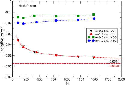
Figure 1: (color online) Relative error in the total energies given by the present functional in comparison with the LDA results. Here we consider Hooke’s atoms with two oscillator strengths. Both self-consistent (SC) and non-self-consistent (NSC) results are shown; in the latter case LDA densities are used as an input. The curves on the SC data represent the best polynomial fit of the type $a+bN^{c}$. The horizontal solid lines represent the asymptotic error for $N\rightarrow\infty$ extrapolated from the above relation.

IV.2 Jellium model

Next we consider the spherical jellium model that has been successfully used to study the electronic structure of metal clusters containing thousands of atoms jellium . The external potential $v_{ext}(r)$ entering Eq. (30) is the Coulomb potential of a homogeneous sphere of radius $R_{b}=N^{1/3}r_{s}$, where $r_{s}=[3/(4\pi\rho)]^{1/3}$ is the Wigner-Seitz radius. The external potential becomes

$$v_{ext}(r)=\left\{\begin{array}[]{ll}-\frac{N}{2R_{b}}\left(3-\frac{r^{2}}{R_{b}^{2}}\right)&\mbox{for }r\leq R_{b}\\ -\frac{N}{r}&\mbox{for }r>R_{b}.\end{array}\right.$$ (32)

For numerical computations we consider the sodium-like case ($r_{s}=4.0$) with $N=169,\,398,\,638$, and $1000$. The results in comparison with the LDA calculations are shown in Fig. 2. In contrast with the results for Hooke’s atoms, the total energies are now overestimated. The relative error of the SC calculations increases as a function of $N$ but – similarly to Hooke’s atoms in the lower panel – the error seems to stabilize in the asymptotic limit to about $10.6\%$. In contrast, the NSC errors remain below $2\%$. Thus, it seems that at least in the non-atomic applications considered here, there is a price to pay with the self-consistency in terms of accuracy, although the stabilization of the error as a function of $N$ is a desirable property. Finally, we point out that the difference in the sign of the error in comparison with the Hooke’s atom is due to the tail of jellium potential ($-N/r$), whereas the center of the system is dominated by a harmonic term.

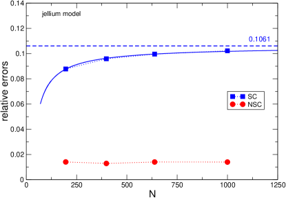
Figure 2: (color online) Relative error in the total energies given by the present functional in comparison with the LDA results in the case of a jellium model. Both self-consistent (SC) and non-self-consistent (NSC) results are shown. The curve on the SC data represents the best polynomial fit of the type $a+bN^{c}$. The horizontal dashed line shows the asymptotic error for $N\rightarrow\infty$ extrapolated from the above relation.

IV.3 Atom-like systems

Finally we consider an atomic potential of the form

$$v_{ext}(r)=-\frac{N}{r+\delta}$$ (33)

with a softening parameter $\delta=1$. This parameter is introduced to make the potential close to the core relatively smooth. This allows all-electron calculations with an analytic basis of spherical Bessel functions. Figure 3 shows the relative errors in the energies for $N=10$, 18, 36, 54, 86, and 118. In this case the performance of the present functional is very good: in small systems up to $N~{}30$ the error remains below $2\%$ and then gradually increases to $5\%$ in the extrapolated limit. Interestingly, the NSC calculation shows slightly worse performance in this case, especially at small $N$.

Overall, the result in Fig. 3 is promising regarding applications in atom-like systems. To improve the accuracy further, the prefactor $\alpha$ in Eq. (25) could be optimized to reproduce the high-$N$ limit exactly. However, here we refrain from such an ad hoc modification. Finally, we note that the obvious lack of size-consistency in the functional prevents straightforward applications to systems consisting of fragments.

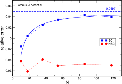
Figure 3: (color online) Relative error in the total energies given by the present functional in comparison with the LDA results in the case of a model atom. Both self-consistent (SC) and non-self-consistent (NSC) results are shown. The curve on the SC data represents the best polynomial fit of the type $a+bN^{c}$. The horizontal dashed line shows the asymptotic error for $N\rightarrow\infty$ extrapolated from the above relation.

V Summary

In summary, we have derived a self-consistent orbital-free functional for the total ground-state energy of arbitrary three-dimensional electronic systems. In the derivation we have applied Parr’s construction parr as a starting point that expresses the total interaction energy in a simple integral form that depends on the number of electrons $N$. We have suggested a modified form of the interaction energy that exploits the Hartree energy in the limit of a constant electron density. Furthermore, we have used the variational principle to derive an explicit expression for the electron density. As a result, our functional requires only the external potential and $N$ as input parameters and produces the total energy with an almost negligible computational cost.

We have tested the functional for different systems including Hooke’s atoms, jellium models, and atomic potentials. Reasonable agreement with the total energies of the local-density approximation has been found in all cases, and in atomic systems the accuracy is particularly good. Importantly, the relative errors in the total energy become constant in the large-$N$ limit in all systems. This tendency suggests to modify the prefactor of the total energy expression. Even better, it might be possible to density-functionalize the prefactor through scaling relations of the Thomas-Fermi theory. It should be noted that the main benefit of the present functional over the Thomas-Fermi method is the computational simplicity, as the chemical potential is the only parameter to be determined according to the normalization. Otherwise the functional is explicit and free from the Hartree integral.

We find the greatest promise of the present functional in total energy calculations of large electronic systems described by various external potentials, e.g., large metallic clusters, spherical semiconductor quantum dots, or electron gas confined by attractive Coulomb potential. Naturally, in these applications the asymptotic tendency to slightly under- or overestimate the energy needs to be taken into account by a possible additional modification. Due to the minimal comptational cost the functional can be also applied in a qualitative manner to estimate the energetic properties of very large, even macroscopic electronic systems.

- (1) L. Hung and E. A. Carter, Chem. Phys. Lett. 475, 163 (2009).
- (2) Y. A. Wang and E. A. Carter, Theoretical Methods in Condensed Phase Chemistry, in series Progress in Theoretical Chemistry and Physics, Ed. S. D. Schartz, pp. 117 (Kluwer, Dordrecht, 2000); V. L. Ligneres and E. A. Carter, An introduction to orbital-free density functional theory, (Springer, Netherlands, 2005).
- (3) R. G. Parr, J. Chem. Phys. 92, 3060 (1988).
- (4) S. Pittalis and E. Räsänen, Phys. Rev. B 80, 165112 (2009).
- (5) E. Räsänen, S. Pittalis, G. Bekcioglu, and I. Makkonen, Phys. Rev. B 87, 035144 (2013).
- (6) S. R. Gadre, L. J. Bartolotti, and N. C. Handy, J. Chem. Phys. 72, 1034 (1980).
- (7) E. H. Lieb and S. Oxford, Int. J. Quantum Chem. 19, 427 (1981).
- (8) E. Räsänen, S. Pittalis, K. Capelle, and C. R. Proetto, Phys. Rev. Lett. 102, 206406 (2009).
- (9) E. Räsänen, M. Seidl, and P. Gori-Giorgi, Phys. Rev. B 83, 195111 (2011).
- (10) I. Makkonen, M. M. Ervasti, V. J. Kauppila, and A. Harju, Phys. Rev. B 85, 205140 (2012).
- (11) J. P. Perdew and A. Zunger, Phys. Rev. B 23, 5048 (1981).
- (12) M. Brack, Rev. Mod. Phys. 65, 677 (1993).
- (13) A. Odriazola, A. Delgado and A. González, Phys. Rev. B 78, 205320 (2008).