Guaranteed Collision Detection
With Toleranced Motions

Abstract

We present a method for guaranteed collision detection with toleranced motions. The basic idea is to consider the motion as a curve in the 12-dimensional space of affine displacements, endowed with an object-oriented Euclidean metric, and cover it with balls. The associated orbits of points, lines, planes and polygons have particularly simple shapes that lend themselves well to exact and fast collision queries. We present formulas for elementary collision tests with these orbit shapes and we suggest an algorithm, based on motion subdivision and computation of bounding balls, that can give a no-collision guarantee. It allows a robust and efficient implementation and parallelization. At hand of several examples we explore the asymptotic behavior of the algorithm and compare different implementation strategies.

Keywords: Toleranced motion, collision detection, bounding ball, bounding volumes.

2010 MSC: 65D18, 70B10

1 Introduction

Collision detection between moving solids [1] is an ubiquitous issue in robotics and other fields, such as computer graphics or physics simulation. General-purpose strategies are available as well as algorithms tailored for specific situations. In general, any algorithm is a trade-off between reliability, accuracy, and computation time. In some scenarios, for example in trajectory planning for high-speed heavy robots, collisions might have devastating effects. Therefore, it is necessary to exclude them with certainty. This article presents an efficient algorithm that can give such a guarantee for collisions between polyhedra under certain assumptions on the motion.

Typical techniques of collision detection include time discretization [1, Section 2.4], motion linearization, and the use of bounding volumes [1, Chapter 4] or hierarchies of bounding volumes [1, Chapter 6] and [2, 3]. Careful application of discretization and linearization is critical, as collisions with a short time interval of interference may be missed. The algorithm we propose in this article uses hierarchies of bounding volumes but it exhibits some specialties with respect to their construction. When using bounding volumes, several potentially contradicting requirements have to be fulfilled [1, p. 76]: The computation of the bounding volumes must be efficient, the representation of moving and fixed object by not too many bounding volumes has to be accurate, and the collision queries for bounding volumes should be fast.

In this article, we present ideas for a collision detection algorithm that satisfies these criteria, at least to a certain extent. The novelty is to use a ball covering of the motion which we regard as a curve in the 12-dimensional space of affine displacements. This ball covering can be converted into a system of simple bounding volumes of elementary objects (points, lines, planes, and polygons). Unlike other methods for collision detection based on bounding balls, this requires only the covering of a one-dimensional object (the motion) as opposed to the covering of a 3D-solid. The bounding volumes are constructed from the geometry of the moving object and its motion and thus accurately represent the portion of space occupied by the object as it moves. It is possible to refine the bounding volumes by subdividing the motion. With every subdivision step, the number of bounding volumes doubles while their volume shrinks roughly by the factor $2^{-3}$. This is much better than for ball coverings of non-curve like objects in 3D. Furthermore, the worst case complexity of subdivision is usually not achieved because large parts of motion or moving objects can be pruned away at a low recursion level.

We expect our algorithm to work particularly well for objects that lend themselves to polyhedral approximations. Other desirable properties include:

• The possibility to report approximate time and location of potential collisions,

• simple, fast and robust implementation because of recursive function calls without the need of sophisticated data structures,

• the use of fast and robust primitive procedures which are well-known in computational geometry, and

• the possibility of parallelization.

Assuming a robust numerical implementation, collisions up to a pre-defined accuracy will always be detected correctly and reported non-collisions are guaranteed.

The ball covering in the space of affine displacements is based on an underlying object-oriented Euclidean metric [4, 5] which is derived from a mass distribution in the space of the moving object. This mass distribution already saw applications in computational kinematics, for example [6, 7, 8]. One of its important properties, the simplicity of certain orbit shapes with respect to balls of affine displacements, was observed in [9]. It is our aim, to exploit this for guaranteed collision detection under certain not too restrictive assumptions on the motion.

Since collision detection is a well-explored research topic, we want to compare the algorithm we propose with other approaches known from literature.

There is a number of techniques for detecting collisions or computing the distance of moving objects by means of covering balls or hierarchies of covering balls [10, 2, 11, 12, 3, 13, 14]. We cover the moving objects by different bounding volumes (portions of balls and hyperboloids of one or two sheets). However, our construction is based on a covering of a curve in $\mathbb{R}^{12}$ (the motion) by balls. This latter problem is typically simpler and of lesser complexity than constructing ball coverings for 3D solids. Depending on the particular situation, certain curve specifics, for example piecewise rationality, can be used to efficiently generate systems of bounding balls. In contrast to collision detection with covering balls, our algorithm typically requires exactly one quadratic bounding surface (sphere or hyperboloid) per vertex, edge, and face. As in case of bounding spheres, efficient collision queries are possible by evaluation of quadratic functions only.

Several authors suggest bounding volume shapes which are specifically tailored to the needs of collision detection. Typical examples are the generalized cylinders of [12] and the s-topes of [15]. Usually, they are derived from some ball covering. An s-tope is, for example, the convex hull of a finite set of spheres. These shapes visually resemble our bounding volumes. The crucial difference is that our construction takes into account the objects’ motion in such a way that it is guaranteed to stay within the volume during the whole motion. In this sense, it resembles the space-time solids of [2] or the implementation for jammed random packing of ellipsoids described in [16, 17]. A non-collision guarantee is often possible by means of a coarse representation. Only if a collision cannot be excluded, the bounding volumes are adaptively refined. The prize we pay for this exact collision detection with arbitrary accuracy is the necessity to re-compute the bounding volumes if the motion changes.

It has to be emphasized that our approach requires no time-discretization or motion linearization. We work with the motion as it is analytically defined over a parameter interval. Moreover, our algorithm should not be confused with algorithms for (approximate) distance calculation although it can report whether or not the distance falls beyond a certain threshold during a given motion. Naturally, our algorithm is considerably slower than many of the sophisticated existing algorithms but its outcome is of a high quality. A reported no-collision is guaranteed. Our algorithm should only be used when such a certification is crucial.

The remainder of this article is organized as follows. After presenting some preliminaries about the object-oriented metric in Section 2, we describe the orbits of geometric primitives in Section 3 and their basic collision tests in Section 4. In Section 5 we present some ideas for constructing bounding balls for motions (curves in high-dimensional Euclidean spaces) and in Section 6 we synthesize everything via motion subdivision into a collision detection algorithm. Section 7 presents examples and timing results.

2 Distance between affine displacements

Measuring the “distance” between two displacements is a fundamental problem of computational kinematics with many important applications. It is also afflicted with irresolvable defects such as the incompatibility of units in angle and lengths and dependence on the chosen coordinate frames. For our algorithm, we require a Euclidean metric in the space of Euclidean displacements. Following [4, 5], we equip the space $\mathrm{GA}$+$(3)$ of affine displacements with a left-invariant object-oriented Euclidean metric and embed the Euclidean motion group $\mathrm{SE}(3)$ into $\mathrm{GA}$+$(3)$. After identification of $\mathrm{GA}$+$(3)$ with $\mathbb{R}^{12}$, the Euclidean motion group is a sub-variety of dimension six in this space. The distance concept is based on a positive Borel measure (mass distribution) $\mu$, which defines the scalar product

$$\langle\alpha,\beta\rangle=\int\langle\alpha(x),\beta(x)\rangle\;\mathrm{d}\mu$$ (1)

and the squared distance

$$\operatorname{dist}^{2}(\alpha,\beta)=\langle\alpha-\beta,\alpha-\beta\rangle$$ (2)

for any $\alpha,\beta\in\mathrm{GA}$+$(3)$. In practice, the mass distribution is usually given by a number of feature points $m_{1},\ldots,m_{n}\in\mathbb{R}^{3}$ with positive weights $w_{1},\ldots,w_{n}\in\mathbb{R}_{+}$ whence the scalar product (1) and squared distance (2) become

$$\langle\alpha,\beta\rangle=\sum_{i=1}^{n}w_{i}\langle\alpha(m_{i}),\beta(m_{i})\rangle\quad\text{and}\quad\operatorname{dist}^{2}(\alpha,\beta)=\sum_{i=1}^{n}w_{i}\|\alpha(m_{i})-\beta(m_{i})\|^{2}.$$

On the right-hand sides, we use the usual scalar product and norm in Euclidean three-space $\mathbb{R}^{3}$. In this way, the space $\mathrm{GA}$+$(3)$ is endowed with a Euclidean metric and it makes sense to speak of “balls of affine displacements”.

As usual with distance measures for displacements, there is a degree of arbitrariness in this definition. However, the moving object will often suggest a mass distribution in a natural way and we expect that the algorithm’s performance will only marginally depend on the choice of feature points. Both, angle and distance, depend only on the barycenter $b$ of the mass distribution and its inertia matrix $J=(j_{kl})_{k,l\in\{1,2,3\}}$. These are defined via

$$b:=|\mu|^{-1}\int x\;\mathrm{d}\mu,\quad j_{kl}:=\int x_{k}x_{l}\;\mathrm{d}\mu$$ (3)

where $|\mu|=\int\mathrm{d}\mu$ is the total mass and $x_{k}$ is the $k$-th coordinate of $x\in\mathbb{R}^{3}$. In the discrete case, these formulas become

$$|\mu|=\sum_{i=1}^{n}w_{i},\quad b=|\mu|^{-1}\sum_{i=1}^{n}w_{i}m_{i},\quad J=\sum_{i=1}^{n}w_{i}^{2}m_{i}m_{i}^{T}.$$

The feature points $m_{i}$ and weights $w_{i}$ as well as the mass distribution $\mu$ can always be replaced by equally weighted vertices of the ellipsoid with equation $(x-b)^{T}\cdot J\cdot(x-b)=0$ without changing the metric. This is also true in the continuous case. In spite of the general definition of inner product and distance in $\mathbb{R}^{12}$, their computation is always very efficient.

3 Orbits of points, lines, planes and polygons

The orbit of a point set $X\subset\mathbb{R}^{3}$ with respect to a set $Y\subset\mathbb{R}^{12}$ of affine displacements is the point set $\mathcal{O}_{Y}(X):=\{\alpha(x)\mid x\in X,\ \alpha\in Y\}$. The orbits of points, lines, and planes (“fat” points, lines, and planes) with respect to a ball $B=B_{R}(g)\subset\mathbb{R}^{12}$ (center $g$, radius $R$) of affine displacements have been computed in [9, Section 4]. When summarizing the results from that article we always assume that $g$ is the identity. If this is not the case, the orbit shapes have to be displaced by means of $g$.

The orbit of a point $x=(x_{1},x_{2},x_{3})$ with respect to $B$ is a ball $B_{r}(x)$. Its radius $r$ depends on the radius $R$ of $B$, the point $x$, and the metric in $\mathbb{R}^{12}$. It is given by the formula

$$\varrho^{2}(x)\coloneqq\frac{r^{2}}{R^{2}}=\frac{1}{|\mu|}+\sum_{i=1}^{3}\frac{x_{i}^{2}}{\mu_{i}}$$ (4)

where $\mu_{1},\mu_{2},\mu_{3}$ are the eigenvalues of the inertia matrix (3). We call the function $\varrho(x)$ defined by (4) the distortion rate at $x$. It is constant on ellipsoids with axes parallel to the eigenvectors of the inertia matrix and attains its minimum at the barycenter of the mass distribution. This observation helps to picture the distribution of distortion rate in space.

For sufficiently small $R$, the orbit of a line $X$ with respect to $B$ is bounded by a one-sheeted hyperboloid of revolution $\Phi$ with axis $X$ and the orbit of a plane $\xi$ is bounded by a two sheeted hyperboloid $\Psi$ with plane of symmetry $\xi$. We consider the orbit of the line $X$ at first. There exist a parameterization $x(t)=a+tb$, $\|b\|=1$, $t\in\mathbb{R}$ of $X$ such that

$$\varrho^{2}(a+tb)=\varrho_{0}^{2}+\frac{t^{2}}{\nu^{2}}.$$ (5)

We call the real values $\varrho_{0}$ and $\nu$ the metric data of $X$. Denote by $(x,y,z)$ coordinates in an orthonormal frame with origin $a$ and first basis vector $b$. Then the equation of $\Phi$ reads

$$\Phi\colon\frac{x^{2}}{1-(\nu/R)^{2}}+y^{2}+z^{2}=R^{2}\varrho_{0}^{2}.$$ (6)

This describes a hyperboloid of revolution if $0<R<\nu$.

Similarly, the plane $\xi$ admits a parameterization $x(s,t)=a+sb_{1}+tb_{2}$ with orthonormal vectors $b_{1}$, $b_{2}$ such that

$$\varrho^{2}(a+sb_{1}+tb_{2})=\varrho_{0}^{2}+\frac{s^{2}}{\nu_{1}^{2}}+\frac{t^{2}}{\nu_{2}^{2}}.$$ (7)

The real values $\varrho_{0}$, $\nu_{1}$, and $\nu_{2}$ are the plane’s metric data. In the orthonormal frame with origin $a$ and vector basis $(b_{1},b_{2},b_{1}\times b_{2})$, the equation of $\Psi$ reads

$$\Psi\colon\frac{x^{2}}{1-(\nu_{1}/R)^{2}}+\frac{y^{2}}{1-(\nu_{2}/R)^{2}}+z^{2}=R^{2}\varrho_{0}^{2}.$$ (8)

This is a hyperboloid for $0<R<\min\{\nu_{1},\nu_{2}\}$.

Now we consider the orbit $\mathcal{O}_{P}$ of a simple polygon $P$ with respect to the ball $B$ of affine displacements (“fat polygon”). For sufficiently small radius $R$, it is a solid, bounded by patches of spheres (vertex orbits), one-sheeted hyperboloids of revolution (edge orbits), and a two sheeted hyperboloid $\Psi$ (face orbit). In order to find the boundary curves of these surfaces patches, we consider the balls $\{B_{r}(x)\mid x\in P\}$. Their envelope is precisely $\mathcal{O}_{P}$. Thus, the patch on $\Psi$ that actually contributes to the boundary of $\mathcal{O}_{P}$ is the projection of $P$ onto $\Psi$ via the surface normals. Any point $x$ in the polygon’s plane $\xi$ gives rise to two projected images on $\Psi$ which are symmetric with respect to $\xi$. The patch boundaries on $\Psi$ are the projection of the polygon edges. The following proposition completely describes the projected image of $P$. Its proof is a straightforward calculation.

Proposition 1.

Denote by $\sigma$ the non-uniform scaling

$$(x,y,0)\mapsto\Bigl{(}\frac{a^{2}x}{a^{2}+c^{2}},\frac{b^{2}y}{b^{2}+c^{2}},0\Bigr{)}.$$ (9)

The projection of a polygon $P$ in the plane $z=0$ onto the hyperboloid

$$\Psi\colon\frac{x^{2}}{a^{2}}+\frac{y^{2}}{b^{2}}-\frac{z^{2}}{c^{2}}+1=0$$ (10)

via the surface normals consists of those points $(x,y,z)$ whose orthographic projections $(x,y,0)$ into $z=0$ lie in $\sigma(P)$.

Proposition 1 shows that the boundaries between the individual surface patches on the fat polygon $\mathcal{O}_{P}$ are circular and hyperbolic arcs in planes which are “vertical” over $\xi$. This is illustrated in Figure 1. The left-hand drawing shows the original polygon in thick line-style, its scaled copy (the orthographic back-projection of the patch boundaries) and the relevant circular and hyperbolic arcs.

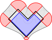
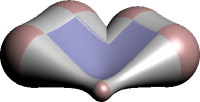
Figure 1: Orbit boundaries for a fat polygon

4 Basic collision tests

The orbits of points, edges and faces with respect to balls of affine displacements are solids bounded by pieces of spheres, hyperboloids of revolutions and hyperboloids of two sheets. In particular, their boundary is composed of piecewise quadratic surfaces and allows to efficiently test for the basic collisions moving vertex vs. fixed face, moving edge vs. fixed edge and moving face vs. fixed vertex ([1, Section 9.1] and [18]). Note that we need not care about “degenerate” collisions (for example edge contained in face) because we use fat points, edges and faces. It is important that the basic collision tests are implemented efficiently and reliably, and that numeric issues must not result in an invalid “no-collision” response. Due to their simple nature, this is possible.

Moving vertex intersects fixed face

Via tolerancing, the moving vertices are converted into balls so that we actually have well-known sphere vs. polygon collision queries [1, Section 5.2.8]. These are especially efficient and simple to implement, if the fixed polygon $F$ is convex.

Moving edge intersects fixed edge

Here we have to test whether a line segment intersects a hyperboloid of revolution between a pair of parallel circles. Note that we do not have to test collision of the line segment with the bounding balls at either end of the moving edge because these are already handled by the preceding test. The intersection problem can be converted into a test whether a quadratic polynomial has zeros in a given interval: Denote by $a$ and $b$ the intersection points of the line segment with the two parallel planes. (Should the original line segment be parallel to the two planes, we have to test whether a similar function has real roots. This is even simpler.) We parameterize the line segment with end points $a$ and $b$ by $\ell(t)=(1-t)a+tb$, $t\in[0,1]$. Plugging $\ell(t)$ into the algebraic equation (6) of the hyperboloid of revolution, we obtain a quadratic equation $q(t)$. The exact test whether it has roots in $[0,1]$ is a trivialization of more advanced algorithms [19].

Moving face intersects fixed vertex

We have to test whether a point $p$ lies between the two sheets of a hyperboloid and whether the orthographic projection of this point lies in the scaled copy $\sigma(P)$ of the moving polyhedron. Here, $\sigma$ is the non-uniform scaling of Equation (9). These two tests amount to determining the sign of a quadratic function at $p$ and a point-in-polygon test [1, Section 5.4.1]. Again, the hyperboloids and balls for edges and vertices can be ignored because their intersections are already handled by preceding tests.

5 Bounding balls for motions

Our collision detection algorithm also requires the computation of a bounding ball for a motion $c(t)$, considered as a curve in $\mathrm{SE}(3)\subset\mathrm{GA}$+$(3)=\mathbb{R}^{12}$. This space is equipped with the object-oriented Euclidean metric derived from a mass distribution $\mu$ in the space of the moving polygon. The problem of finding the (unique) minimal enclosing ball for an arbitrary curve $c(t)$ in a Euclidean space is hard. However, the requirements of our algorithm allow simplifications that make the problem not only tractable but allow efficient solutions in many relevant cases:

• We are not looking for the optimal bounding ball. A “good” approximation is acceptable as well.

• We are allowed to subdivide the curve $c(t)$ and compute bounding balls for the individual segments. If the curvature and arc-length of $c(t)$ can be bounded, after a sufficient number of subdivisions one would assume that the ball over the diameter defined by the curve end-points will bound the complete curve. Below, in Proposition 2 we prove a slightly weaker statement. It gives bounding balls whose radius asymptotically equals half the curve length. For typical motions in robotics, bounds for arc-length and curvature can be obtained if such bounds are known for the joint angles.

• For the important class of piecewise rational motions, the convex hull property allows to use the control polygon for efficient bounding spheres computation.

Here is a simple method to construct bounding balls for short curve segments with small curvature.

Proposition 2.

Let $C$ be a $C^{2}$ curve parameterized by $c\colon[t_{0},t_{1}]\to\mathbb{R}^{d}$ with arc-length $\ell<r\frac{\pi}{2}$ and curvature $\varkappa$ bounded by $|\varkappa|\leq 1/r$. Define $t\coloneqq\ell/r$ and $e_{1}\coloneqq\dot{c}(t_{0})/\lVert\dot{c}(t_{0})\rVert$. Then the complete curve is contained in the ball $B_{k}(m)$ with radius $k=r(1-\cos t)/\sin t$ and center $m=c(t_{0})+ke_{1}$.

The proof of Proposition 2 is based on [9, Lemma 5] which we repeat here for convenience of the reader:

Lemma 1.

Assume that $I\subseteq(-r\frac{\pi}{2},r\frac{\pi}{2})$ is an interval with $0\in I$ and $c\colon I\to\mathbb{R}^{d}$ is an arc length parameterization of a $C^{2}$ curve $C$ with curvature $\varkappa$ such that $|\varkappa|\leq 1/r$. Then there is a parameterization $\overline{c}(u)=ue_{1}+f(u)\cdot n(u)$ of $C$ such that $e_{1}=\dot{c}(0)$, $n(u)$ is a unit vector orthogonal to $e_{1}$, $|u(t)|\geq r\sin(t/r)$ and $|f(u)|\leq r-\sqrt{r^{2}-u^{2}}$.

Figure 2: Bounding ball for curve $c(t)$ with bounded arc length and curvature.

This lemma gives us a bounding volume for the curve $C$:

Lemma 2.

We use the same notation and assumptions as in Lemma 1. In case $d=2$, the curve $C^{\star}$ parameterized by the restriction of $c$ to $[0,t]$ is contained in the area bounded by

• the circular arcs $a$, $\overline{a}$ of radius $r$ and length $t$ which start at $c(0)$ and share the oriented tangent with $C^{\star}$ in this point and

• the segments $i$, $\overline{i}$ of involutes to these circular arcs which connect the point $c(0)+te_{1}$ with the arc end points $e$, $\overline{e}$

(Figure 2). In case of $d>2$, the curve $C^{\star}$ is contained in the volume obtained by rotating this area about the curve tangent in $c(0)$.

Proof.

We consider the case $d=2$ first. Lemma 1 implies that the curve point $c(t)$ lies in the exterior of the two circles through $a$, $\overline{a}$. Because of the bounded arc length $t$, the curve will not go beyond the circular involutes $i$, $\overline{i}$. If $d>2$, the claim follows by considering the graph of the function $f(u)$ in the plane spanned by $e_{1}$ and $e_{2}=n(0)$. ∎

Proof of Proposition 2.

The curve $C$ has an arc-length parameterization that satisfies the criteria of Lemma 1. Hence, we can enclose it in the volume given by Lemma 2. In order to prove the proposition, we have to show that the ball $B_{k}(m)$ contains this volume. Center $m$ and radius $k$ are chosen such that the start points $c(t_{0})$, $e$ and $\overline{e}$ of curve and involutes lie on the ball boundary. It is a little tedious but possible to verify that it also contains the involute arcs $i$, $\overline{i}$ for any value $\ell\in[0,r\frac{\pi}{2}]$ (Figure 2). ∎

6 Collision detection algorithm

Now we sketch an algorithm for collision detection by means of toleranced motions. We describe only the case of collisions between a fixed polygon $F$ and a moving polygon $P$, undergoing a motion $c(t)$. These polygons are assumed to be simple and we think of them as being composed of vertices, edges, and one face. For the actual implementation, it is advantageous to have access to lists of vertices and edges. Collision detection for the case of polyhedra can be reduced to this situation.

The basic idea of motion tolerancing is to cover a given one-parametric motion by a sequence of full-dimensional motions and then test the orbits of geometric entities (balls, straight-line segments, polygons) with respect to these full-dimensional motions for collision. If no collision occurs, it can also be excluded for the originally given motion. If this is not the case, the sequence of covering motions needs to be refined.

The motion $c(t)$ is a curve on $\mathrm{SE}(3)\subset\mathrm{GA}$+$(3)=\mathbb{R}^{12}$, defined over an interval $I=[t_{0},t_{1}]$. We assume that we can compute a “small” bounding ball for the restriction of $c(t)$ to any sub-interval of $I$. Here, the words “ball” and “small” refer to the object-oriented Euclidean metric in $\mathbb{R}^{12}$, induced via a positive Borel measure $\mu$ in the space of the moving polygon (Section 2).

We start our algorithm by a pre-processing step where we compute for every edge $e_{i}$ of the moving polygon $P$ and for the plane $\xi$ of $P$ the metric data as defined by (5) and (7). This gives us a pair $(\nu_{i},\varrho_{0,i})$ for every edge and a triple $(\nu^{\prime}_{1},\nu^{\prime}_{2},\rho_{0})$ for $\xi$. From a computational point of view, this amounts to the principal axis transform of a one- or two-dimensional quadric. Transcendental functions are involved only at this stage of the algorithm. Since the metric data depends only on the moving polygon $P$ and the Borel measure $\mu$, it can be re-used for different motions $c(t)$ and different fixed polygons $F$.

In the algorithm itself, we construct a bounding ball $B_{R}(g)$ of $c(t)$ and test the toleranced moving polygon $P$ with respect to this ball for collision with the fixed polygon $F$. The necessary tests are described in Section 4. We perform them with respect to a certain “zero-position” of $P$ in the plane with equation $z=0$. This requires the prior transformation of $F$ via $g^{-1}$. In return for the necessary inversion of a $3\times 3$ matrix we get an easier and cleaner implementation. If the orbit of $P$ with respect to $B_{R}(g)$ intersects $F$, we recursively subdivide the motion $c(t)$ and repeat the collision test. If a “no-collision” predicate cannot be given before the termination criterion, the algorithm returns a time interval of possible collisions. Otherwise, if no collision occurs, it returns an empty interval. It is possible to add information on the location and type of collision. Moreover, the sub-tasks obtained from the repeated subdivision of $c(t)$ can be solved in parallel.

We suggest to terminate this recursive algorithm as soon as the product

$$R_{\min}\coloneqq R\max_{x\in P}\varrho(x)$$ (11)

of current bounding ball radius $R$ and maximal distortion rate attained inside the moving polygon is smaller than a pre-defined value $\varepsilon>0$. Pre-computing this value amounts to solving a quadratic program. With this termination criterion only sub-motions that bring the two polygons within a distance of $\varepsilon$ to each other remain without a no-collision guarantee. Given the limited accuracy of robot motion, this is probably desirable anyway.

Listing 1 Collision detection; returns list of possibly colliding elements or empty list in case of no collision.

procedure Collision($P,F,c,d$) $\triangleright$ moving polygon $P$, fixed polygon $F$,

motion $c$, recursion depth $d$

     if $d=0$ then

         return parameter interval of $c$ $\triangleright$ too many recursions

     end if

     $g,R\leftarrow\textsc{BoundingBall}(c)$ $\triangleright$ center $g$, radius $R$

     if $R<R_{\min}$ then $\triangleright$ see Equation (11)

         return parameter interval of $c$ $\triangleright$ radius too small

     end if

     if $\textsc{Intersection}(P,F,g,R)$ then $\triangleright$ see Listing 2 below

         $c^{\prime},c^{\prime\prime}\leftarrow\textsc{Subdivide}(c)$

         return Collision($P,F,c^{\prime},d-1$)

         return Collision($P,F,c^{\prime\prime},d-1$)

     else

         return $[]$ (empty list) $\triangleright$ no collision

     end if

end procedure

Listing 2 Intersection of fat moving polygon, determined by moving polygon and ball $B_{R}(g)\subset\mathbb{R}^{12}$, and fixed polygon.

procedure Intersection($P,F,g,R$) $\triangleright$ moving polygon $P$, fixed polygon $F$,

center $g$ and radius $R$

Metric data of plane of $P$ and edges of $P$ has been pre-computed and is accessible from within this procedure.

     $P^{\prime}\leftarrow\textsc{FatPolygon}(\mathrm{id},R)$ $\triangleright$ fat polygon in “zero position”

     $F^{\prime}\leftarrow g^{-1}(F)$

     for each fat vertex $x$ of $P^{\prime}$ do $\triangleright$ ball intersects polygon

         if $x$ intersects $F^{\prime}$ then

              return true

         end if

     end for

     for each fat edge $e$ of $P^{\prime}$ do $\triangleright$ line segment intersects hyperboloid

         for each edge $f$ of $F^{\prime}$ do

              if $e$ intersects $f$ then

                  return true

              end if

         end for

     end for

     for each vertex $y$ of $F^{\prime}$ do $\triangleright$ point in hyperboloid, point projection in polygon

         if $y$ lies in fat face of $P^{\prime}$ then

              return true

         end if

     end for

     return false

end procedure

The complete algorithm in pseudo-code is displayed in Listings 1 and 2. The first call of procedure Collision($P,F,c,d$) should have the complete vertex, edge and face lists of both, moving and fixed polygon as arguments. A limit on the recursion depth is good programming practice but, from a theoretical point of view, not necessary.

Remark 1.

At this point we would like to mention one implementation detail we have not explained so far: It is possible that the radius $R$ of the bounding ball $B_{R}(g)$ is so large that the fat edge or face is no longer bounded by a hyperboloid, compare Equations (6) and (8). The simplest method to circumvent this problem is to subdivide the motion and thus decrease the ball radius $R$. But it is also possible to exploit this behavior for simplified collision tests:

• If the inequality $R\geq\nu_{i}$ holds for edge $e_{i}$, the fat edge is contained in the union of the two fat points over its end-points. Thus, we may be able to exclude a collision by testing for the intersection of a line segment with balls [1, Section 5.3.2].

• If $\max\{\nu^{\prime}_{1},\nu^{\prime}_{2}\}\leq R$, the fat vertices of the moving polygon envelope the complete fat polygon. The collision between $P$ and $F$ can be tested by solely checking possible intersections of $F$ with these vertex balls [1, Section 5.2.8].

• If either $\nu^{\prime}_{1}\leq R\leq\nu^{\prime}_{2}$ or $\nu^{\prime}_{2}\leq R\leq\nu^{\prime}_{1}$ hold, the vertex spheres not necessarily envelope the toleranced position of $F$. By the Cauchy interlacing theorem [20], there exist two straight lines in the plane of $P$ through the point of minimal distortion rate that divide the plane into four regions. In the interior of each of these regions, the situation is either as in the case $\nu^{\prime}_{1},\nu^{\prime}_{2}\leq R$ or as in the case $\nu^{\prime}_{1},\nu^{\prime}_{2}\geq R$ and can be handled accordingly. Should $P$ overlap two or more regions we may subdivide $P$.

Remark 2.

Finally, we would like to point out a possibility to considerably speed up the algorithm if the recursive subdivision and bounding ball construction for the motion $c(t)$ produces a nested ball covering, that is, a ball covering where the balls after subdivision are contained in the ball before subdivision. In this case, it is sufficient to test only those elements for collision for which a collision at a preceding recursion level could not be excluded. It is possible to incorporate this in the presented algorithm by maintaining lists of vertices, edges and faces that still require collision testing. Methods for generating nested ball coverings are available [10]. Their applicability in our algorithm depends on the type of motion we consider.

7 Examples and timings

In this section, we describe a couple of examples in more detail. The first group of examples considers a single fixed and a single moving polygon that undergoes two different motions, one with collision, the other without. The second group of examples is designed to demonstrate the asymptotic behavior of our algorithm. We consider the collision of two squares after subdivision into $n^{2}$ sub-squares.

The reader will notice that we always consider convex polygons. This simplifies the implementation, in particular the collision test of moving vertex and fixed face. Non-convex faces can always be decomposed into convex parts. The impact on the overall performance should be small.

For the computation of examples we used a personal computer with an Intel Core 2 Duo CPU with 3000 MHz, 8 GB system memory and a 64-bit Ubuntu 14.04. Programming language for this simple implementation is C++, the code was compiled using g++ in version 4.8.2.

7.1 Collision of one fixed and one moving polygon

In this section we consider two different motions of a moving polygon $P$ and its possible collisions with a fixed polygon $F$ (see Figures 4 and 4). The polygons $P$ and $F$ are convex octagons. During the first motion, the two polygons do not collide, during the second motion, they do. In both cases, the motion is rational of degree eight. In fact, the motions differ only by a constant translation. The Borel measure is derived from point masses of equal weight in the vertices of the moving polygon $P$ and in a point over the barycenter of $P$ with comparably small distance to the plane of $P$. This ensures that a scaled copy of the inertia ellipsoid roughly captures the shape of $P$.

The motion is a rational Bézier curve $c(t)$ of degree eight in $\mathrm{GA}$+$(3)=R^{12}$ with positive weights. We use the curve point $g\coloneqq c(0.5)$ as center of a bounding ball $B_{R}(g)$ and choose the radius $R$ as the maximal distance to a control point. Should this ball be too large to exclude collisions, we subdivide the curve by means of de Casteljau’s algorithm, compute bounding balls for both parts and test again for collisions. This procedure we repeat until we can exclude a collision or until we reach the termination criterion described in Section 6.

It would be possible to use different strategies for computing bounding balls, for example the minimal bounding ball of the control polygon [21] or an approach inspired by Proposition 2. We don’t expect much difference but remark that neither approach is guaranteed to produce a nested ball covering. Thus, we cannot profit from pruning away non-colliding objects from previous stages. We did not implement a special handling for balls of large radius as explained in Remark 1 but simply subdivide in this case.

In the first example, a collision can be excluded. The total computation time minus the time for pre-processing is 0.1427 seconds. The maximal recursion depth is eight but only 173 collision tests polygon vs. fat polygon are performed. From Figure 4 we can infer that excluding a collision in this example is rather difficult because the moving polygon is always “near” the fixed polygon. If we translate the moving polygon by about half of its diameter away from the fixed polygon, the computation is roughly half as long.

In the second example, the two polygons interfere during a time interval. We require a maximum of eight recursions and 0.0075 seconds until we reach the termination criterion. The value of $\varepsilon$ is set to about one percent of the polygon diameters. A total of nine collision tests polygon vs. fat polygon are performed.

Figure 3: Motion of $P$ in Example 1

Figure 4: Motion of $P$ in Example 2

7.2 Experiments on asymptotic behavior

Now we consider the potential collision of two polyhedral surfaces that were obtained from two squares by subdivision into $n^{2}$ sub-squares. Thus, we have $n^{4}$ collision tests of moving vs. fixed polygon. Of course this example is artificial but the algorithm does not profit at all from the regular structure so that conclusions for large polyhedral surfaces in general seem justified.

The two subdivided squares undergo three different rational motions of degree eight: One with a collision, one with a near-collision and one with a “clear” no-collision. The rotational component of these motions is always the same, they differ only in a constant translation. We run the algorithm for $1\leq n\leq 10$ until we have a no-collision guarantee or reach the termination criterion of the previous examples. The recorded data is the total time (average over 100 runs), the total time per moving polyhedron (that is, collision of one moving square with $n^{2}$ fixed squares) and the average time of one collision test square vs. square.

Finally, we distinguish between two different strategies: We either use one global mass distribution for the complete moving polyhedral surface or we compute an individual mass distribution for each moving square. The aim is to explore whether the additional computational burden of the latter strategy is compensated by the faster detection of a non-collision.

	Collision		Near-Collision		No-Collision
$n$	total [s]	average [s]	total [s]	average [s]	total [s]	average [s]
1	0.17	0.17	0.49	0.49	0.11	0.11
2	1.58	0.10	2.43	0.15	1.12	0.07
3	5.91	0.07	9.49	0.12	4.57	0.06
4	16.07	0.06	25.78	0.10	12.17	0.05
5	35.09	0.06	57.05	0.09	27.60	0.04
6	67.41	0.05	110.34	0.09	54.82	0.04
7	118.42	0.05	193.47	0.08	98.25	0.04
8	194.16	0.05	318.39	0.08	164.00	0.04
9	300.88	0.05	494.69	0.07	258.29	0.04
10	448.09	0.04	738.22	0.07	388.67	0.04

Table 1: Test data for collision, near-collision and no-collision with a global mass distribution

	Collision		Near-Collision		No-Collision
$n$	total [s]	average [s]	total [s]	average [s]	total [s]	average [s]
1	0.17	0.17	0.49	0.49	0.11	0.11
2	1.21	0.07	1.85	0.12	0.98	0.06
3	3.68	0.04	5.99	0.07	3.22	0.04
4	9.12	0.04	15.23	0.06	8.27	0.03
5	19.01	0.03	32.59	0.05	18.74	0.03
6	35.69	0.03	62.36	0.05	36.97	0.03
7	61.59	0.03	108.64	0.04	66.01	0.03
8	99.71	0.02	177.00	0.04	109.79	0.03
9	153.22	0.02	274.48	0.04	172.29	0.03
10	226.60	0.02	407.89	0.04	258.99	0.03

Table 2: Test data for collision, near-collision and no-collision with individual mass distributions

The data for total and average time is displayed in Table 1 for a global mass distribution and in Table 2 for individual mass distributions. The total time per moving polygon is visualized in Figure 5 for a global mass distribution and in Figure 6 for individual mass distributions. In these figures, we plot the time per moving square as a histogram over the moving squares. The height of each box is proportional to the time for excluding a collision or reaching the termination criterion without a no-collision guarantee. The latter case is indicated by a colored box. We see that collisions or near-collisions occur only at one corner and observe an increase of computation time in the vicinity of this corner.

	$n=1$	$n=4$	$n=7$	$n=10$
collision
yes
near
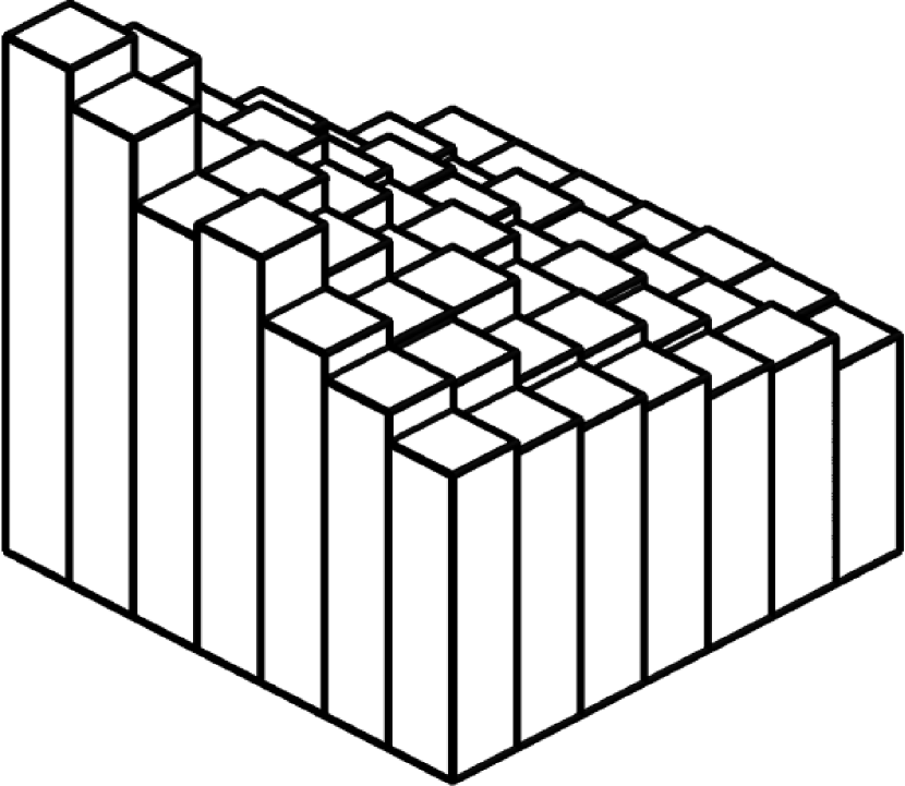
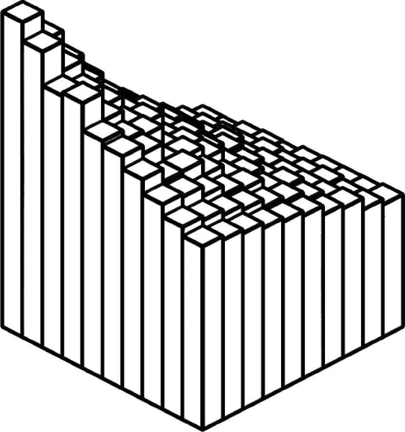
no

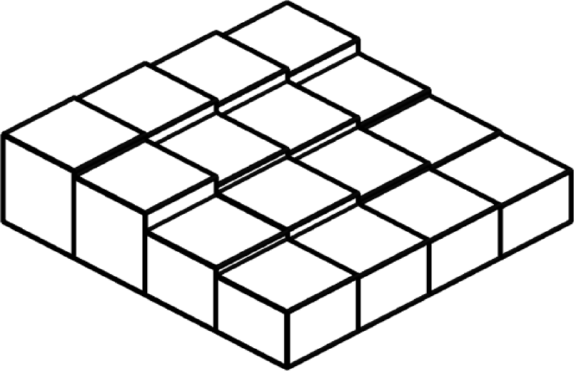
Figure 5: Time per moving square with a global mass distribution

	$n=1$	$n=4$	$n=7$	$n=10$
collision
yes
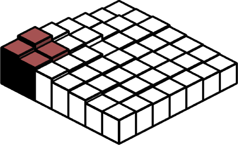
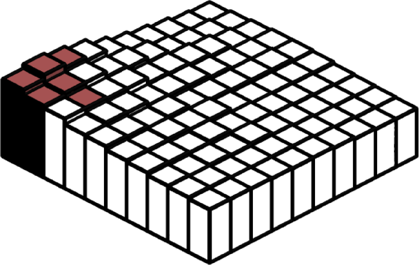
near
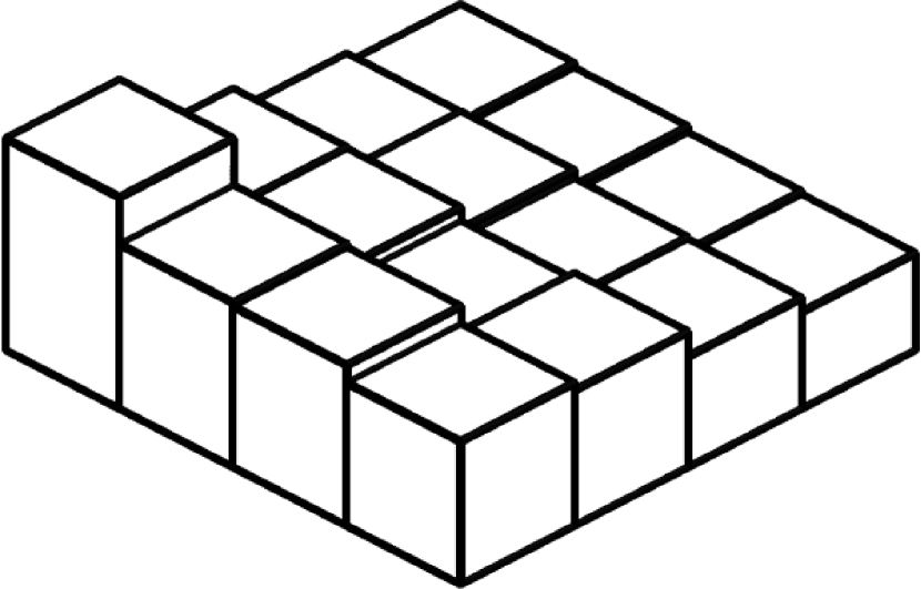
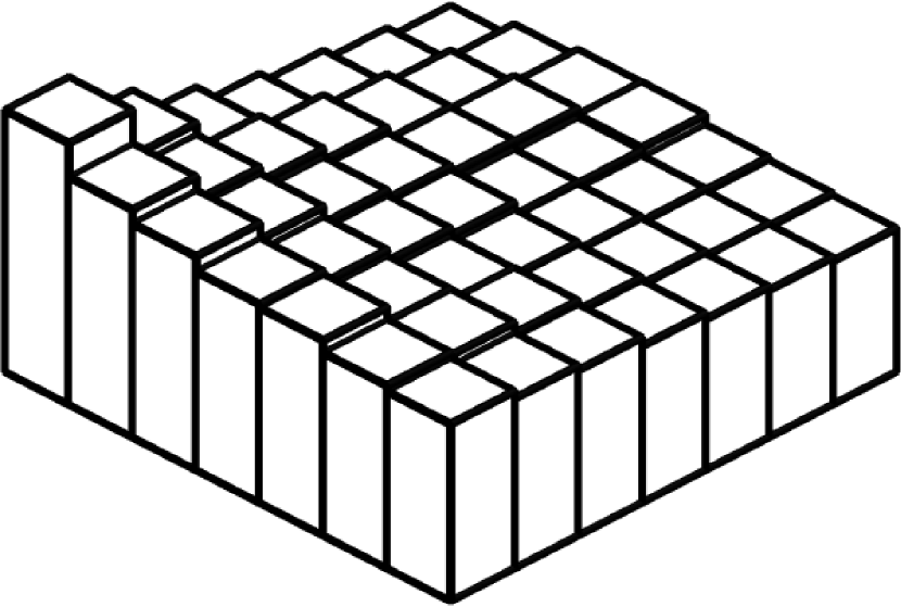
no

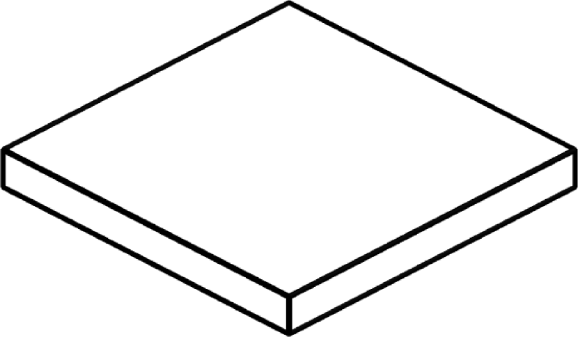
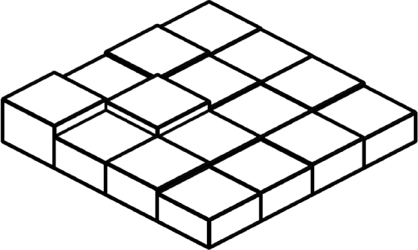
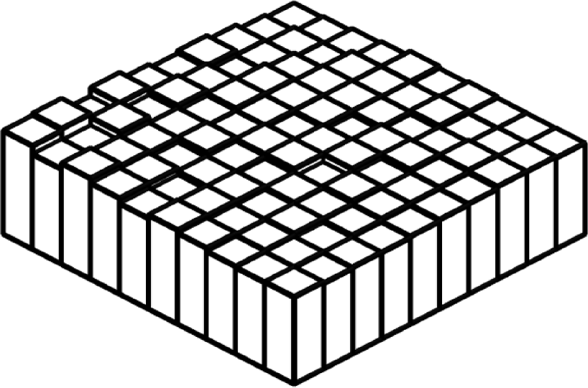
Figure 6: Time per moving square with individual mass distributions

The examples of this section allow to draw the following conclusions:

• The asymptotic behavior is linear in the total number $n^{4}$ of collision tests. This is to be expected since large $n$ means also a large number of no-collisions. The total time roughly equals the average time for the exclusion of a collision times the number of intersection tests for two polygons.

• It is better to use individual mass distributions, in particular in the presence of collisions. The reason is that the time for computing the mass distribution is negligible but very often speeds up the detection of a non-collision. The ratio of total times is between approximately 1.5 in case of no collision and 2.0 in case of a collision. This is probably because many near-collisions in the latter case are recognized as no-collisions at a lower recursion depth.

• The algorithm can greatly profit from a hierarchy of bounding polyhedra. This is nicely illustrated by Figures 5 and 6. In order to give a no-collision guarantee, it is sufficient to subdivide only the squares that, at a given recursion depth, correspond to colored boxes. At least in our examples, large parts of the polyhedral surface can be pruned away at low recursion depths.

8 Concluding remarks

In this paper we exploited the simple orbit shape of points, lines, planes and polygons with respect to balls $B_{R}(g)\subset\mathbb{R}^{12}$ of affine displacements for an efficient collision detection algorithm. Emphasis is put on reliable no-collision guarantee, simple implementation and fast detection of intervals with no collision. A prototype implementation demonstrates that real-time collision detection for reasonably simple polyhedral shapes undergoing a rational motion is possible, provided there are few expected collisions or near-collisions.

Our algorithm works with affine deformations while for many of the envisaged applications just rigid body displacements are required. Thus, one might wonder whether something could be gained by a restriction to Euclidean motions. However, the tolerancing analysis in [9] gives no evidence for this believe. Linearization of $\mathrm{SE}(3)\subset\mathrm{GA}$+$(3)$ and subsequent error estimation comes at the cost of more complicated orbit shapes. For example, the orbits of points with respect to the intersection of a ball with $\mathrm{SE}(3)$ are contained in offsets to ellipsoids. Collision tests with these surfaces are so much harder than with balls that one is certainly willing to accept more recursions instead.

A necessary ingredient in our algorithm is the possibility to efficiently generate bounding balls for curve segments. We already remarked that for sufficiently short curves of small curvature one can probably use the ball for which the curve end points are antipodal. It would be good to have a more precise statement. Moreover, we emphasize the need for efficient algorithms that generate nested ball coverings for motions of technical relevance, in particular piecewise rational motions. This is topic of future research.

References

- [1] C. Ericson, Real-Time Collision Detection, Morgan Kaufman, 2005.
- [2] P. M. Hubbard, Collision detection for interactive graphics applications, IEEE Trans. Visualization and Computer Graphics 1 (3) (1995) 218–230.
- [3] J. Dingliana, C. O’Sullivan, Graceful degradation of collision handling in physically based animation, Eurographics 19 (3) (2000) 239–248.
- [4] C. Belta, V. Kumar, An SVD-based projection method for interpolation on SE(3), IEEE Transactions on Robotics and Automation 18 (3) (2002) 334–345.
- [5] G. S. Chirikjian, S. Zhou, Metrics on motion and deformation of solid models, ASME J. Mechanical Design 120 (2) (1998) 252–261.
- [6] M. Hofer, H. Pottmann, B. Ravani, From curve design algorithms to the design of rigid body motions, The Visual Computer 20 (5) (2004) 279–297.
- [7] G. Nawratil, New performance indices for 6R robots, Mech. Machine Theory 42 (11) (2007) 1499–1511.
- [8] H.-P. Schröcker, B. Jüttler, M. Aigner, Evolving four-bars for optimal synthesis, in: M. Ceccarelli (Ed.), Proceedings of EUCOMES 08, Springer, 2009, pp. 109–116. doi:10.1007/978-1-4020-8915-2.
- [9] H.-P. Schröcker, J. Wallner, Curvatures and tolerances in the Euclidean motion group, Results Math. 47 (2005) 132–146.
- [10] S. Quinlan, Efficient distance computation between non-convex objects, in: Proceedings of IEEE Conference on Robotics and Automation, Vol. 4, San Diego, United States, 1994, pp. 3324–3329. doi:10.1109/ROBOT.1994.351059.
- [11] M. Greenspan, K. Burtnyk, Obstacle count independent real-time collision avoidance, in: Proceedings of IEEE International Conference on Robotics and Automation, Minneapolis, Minnesota, US, 1996, pp. 1073–1080.
- [12] B. Martínez-Salvador, A. P. del Pobil, M. Pérez-Francisco, Very fast collision detection for practical motion planning part I: The spatial representation, in: Proceedings of IEEE Conference on Robotics and Automation, Leuven, Belgium, 1998, pp. 624–629.
- [13] R. Weller, G. Zachmann, A unified approach for physically-based simulations and haptic rendering, in: Proceedings of the 2009 ACM SIGGRAPH Symposium on Video Games, Sandbox ’09, ACM, New York, NY, USA, 2009, pp. 151–159. doi:10.1145/1581073.1581097.
- [14] R. Weller, G. Zachmann, Inner sphere trees for proximity and penetration queries, in: 2009 Robotics: Science and Systems Conference (RSS), Seattle, WA, USA, 2009.
- [15] E. J. Bernabeu, J. Tornero, M. Tomizuka, Collision prediction and avoidance amidst moving objects for trajectory planning applications, in: Proceedings of IEEE Conference on Robotics and Automation, Seoul, Korea, 2001, pp. 3801–3806.
- [16] A. Donev, S. Torquato, F. H. Stillinger, Neighbor list collision-driven molecular dynamics for nonspherical hard particles: I. Algorithmic details, Journal of Computational Physics 202 (2005) 737–764.
- [17] A. Donev, S. Torquato, F. H. Stillinger, Neighbor list collision-driven molecular dynamics for nonspherical hard particles: II. Applications to ellipses and ellipsoids, Journal of Computational Physics 202 (2005) 765–793.
- [18] M. Moore, J. Wilhelms, Collision detection and response for computer animation, Computer Graphics 22 (4) (1988) 289–298.
- [19] F. Rouillier, P. Zimmerman, Efficient isolation of polynomial’s real roots, J. Comput. Appl. Math. 162 (2004) 33–50.
- [20] S.-G. Hwang, Cauchy’s interlace theorem for eigenvalues of hermitian matrices, Amer. Math. Monthly 111 (2) (2004) 157–159.
- [21] E. Welzl, Smallest enclosing disks (balls and ellipsoids), in: New Results and New Trends in Computer Science, Vol. 555 of Lecture Notes in Computer Science, Springer, 1991, pp. 359–370.