Analysis of the limiting spectral measure
of large random matrices
of the separable covariance type

Abstract.

Consider the random matrix $\Sigma=D^{1/2}X\widetilde{D}^{1/2}$ where $D$ and $\widetilde{D}$ are deterministic Hermitian nonnegative matrices with respective dimensions $N\times N$ and $n\times n$, and where $X$ is a random matrix with independent and identically distributed centered elements with variance $1/n$. Assume that the dimensions $N$ and $n$ grow to infinity at the same pace, and that the spectral measures of $D$ and $\widetilde{D}$ converge as $N,n\to\infty$ towards two probability measures. Then it is known that the spectral measure of $\Sigma\Sigma^{*}$ converges towards a probability measure $\mu$ characterized by its Stieltjes Transform.
In this paper, it is shown that $\mu$ has a density away from zero, this density is analytical wherever it is positive, and it behaves in most cases as $\sqrt{|x-a|}$ near an edge $a$ of its support. In addition, a complete characterization of the support of $\mu$ is provided.
Aside from its mathematical interest, the analysis underlying these results finds important applications in a certain class of statistical estimation problems.

1. Introduction and problem statement

Consider the $N\times n$ random matrix $\Sigma_{n}=D_{n}^{1/2}X_{n}\widetilde{D}_{n}^{1/2}$ where $X_{n}$ is a $N\times n$ real or complex random matrix having independent and identically distributed elements with mean zero and variance $1/n$, the $N\times N$ matrix $D_{n}$ is determinisitic, Hermitian and nonnegative, and the $n\times n$ matrix $\widetilde{D}_{n}$ is also deterministic, Hermitian and nonnegative. We assume that $n\to\infty$ and $N/n\to c>0$, and we denote this asymptotic regime as “$n\to\infty$”. We also assume that the spectral measures of $D_{n}$ and $\widetilde{D}_{n}$ converge respectively towards the probability measures $\nu$ and $\tilde{\nu}$ as $n\to\infty$. We assume that $\nu\neq\boldsymbol{d}_{0}$ and $\tilde{\nu}\neq\boldsymbol{d}_{0}$ where $\boldsymbol{d}_{x}$ the Dirac measure at $\{x\}$. Many contributions showed that the spectral measure of $\Sigma_{n}\Sigma_{n}^{*}$ converges to a deterministic probability measure $\mu$ and provided a characterization of this limit measure under various assumptions [8, 19, 4, 11], the weakest being found in [22]. In this work, we show that $\mu$ has a density away from zero, this density is analytical wherever it is positive, and it behaves as $\sqrt{|x-a|}$ near an edge $a$ of its support for a large class of measures $\nu$, $\tilde{\nu}$. We also provide a complete characterization of this support along with a thorough analysis of the master equations relating $\mu$ to $\nu$ and $\tilde{\nu}$. To that end, we follow the general ideas already provided in the classical paper of Marchenko and Pastur [15] and further developed in [20] and [5].
In [20], Silverstein and Choi performed this study in the so called sample covariance matrix case where $\widetilde{D}_{n}=I_{n}$. The outline of the present article closely follows that of [20] although at multiple occasions our proofs depart from those of [20], making the article more self-contained. In particular, while Silverstein and Choi benefited from the existence of an explicit expression for the inverse of the Stieltjes transform of $\mu$ when $\widetilde{D}_{n}=I_{n}$, this is no longer the case in the general setting requiring the use of more fundamental analytical tools. In the setting of [20], it has been further shown in [1] that under some conditions, no closed interval outside the support of $\mu$ contains an eigenvalue of $\Sigma_{n}\Sigma_{n}^{*}$, with probability one, for all large $n$. In [2], a finer result on the so called “exact separation” of the eigenvalues of $\Sigma_{n}\Sigma_{n}^{*}$ between the connected components of the support of $\mu$ is shown. Recently, it has been discovered that the characterization in [20] of the support of $\mu$ and the results on the master equations relating $\mu$ to $\nu$, beside their own interest, lead in conjunction with the results of [1, 2] to the design of consistent statistical estimators of some linear functionals of the eigenvalues of $D_{n}$ or projectors on the eigenspaces of this matrix. Such estimators have been developed by Mestre in [16, 17], the initial idea dating back to the work of Girko (see e.g. [9]).
In [5], Brent Dozier and Silverstein studied the properties of the limit spectral measure of the so called “Information plus Noise” ensemble. A first result on the absence of eigenvalues outside the support of the limit spectral measure has been established in [3]. In [14, 10, 21] other separation results as well as statistical estimation algorithms along the lines of [16, 17] were proposed.
Turning to the separable covariance matrix ensemble of interest here, the absence of eigenvalues outside the support of $\mu$ has been established by Paul and Silverstein in [18] without characterizing this support. The results of this paper therefore complement those of [18]. More importantly, similar to the case $\widetilde{D}_{n}=I_{n}$, these results are a necessary first step to devise statistical estimation algorithms of e.g. linear functionals of the eigenvalues of one of the matrices $D_{n}$ or $\widetilde{D}_{n}$. Work on this subject is currently in progress.
Finally, it has been noticed in the large random matrix community that there is an intimate connection between the square root behavior of the density of the limit spectral measure at the edges of the support and the Tracy-Widom fluctuations of the eigenvalues near those edges (see [6] dealing with the sample covariance matrix case). It can be conjectured that such behaviour still holds (with some assumptions on the probability law of the elements of $X_{n}$) in the separable covariance case considered here. In this regard, Theorem 3.3 may help guessing the exact form of the Tracy-Widom law at the edges of the support of $\mu$.

We now recall the results describing the asymptotic behavior of the spectral measure of $\Sigma_{n}\Sigma_{n}^{*}$.

1.1. The master equations

We recall that the Stieltjes Transform of a probability measure $\pi$ on $\mathbb{R}$ is the function

$$f(z)=\int\frac{1}{t-z}\pi(dt)$$

defined on $\mathbb{C}_{+}$. The function $f(z)$ is i) holomorphic on $\mathbb{C}_{+}=\{z\,:\,\Im(z)>0\}$, ii) it satisfies $f(z)\in\mathbb{C}_{+}$ for any $z\in\mathbb{C}_{+}$, and iii) $\lim_{y\to\infty}|yf(\imath y)|=1$. In addition, if $\pi$ is supported by $\mathbb{R}_{+}=[0,\infty)$, then iv) $zf(z)\in\mathbb{C}_{+}$ for any $z\in\mathbb{C}_{+}$. Conversely, it is well known that any function $f(z)$ satisfying i)–iv) is the Stieltjes Transform of a probability measure supported by $\mathbb{R}_{+}$ [13]. Finally, observe that the Stieltjes Transform of $\pi$ can be trivially extended from $\mathbb{C}_{+}$ to $\mathbb{C}-\operatorname*{supp}(\pi)$ where $\operatorname*{supp}(\pi)$ is the support of $\pi$.
In this paper, a small generalization of this result will be needed [13, Appendix A]: The three following statements are equivalent:

• The function $f(z)$ satisfies the properties i), ii), and iv),

• It admits the representation

  $$f(z)=a+\int_{0}^{\infty}\frac{1}{t-z}\pi(dt)$$

  where $a\geq 0$ and where $\pi$ is a Radon positive measure on $\mathbb{R}_{+}$ such that $0<\int_{0}^{\infty}(1+t)^{-1}\pi(dt)<\infty$,

• The function $f(z)$ satisfies the properties i) and ii), and furthermore, it is analytical and nonnegative on the negative real axis $(-\infty,0)$.

We now recall the first order result.

Proposition 1.1 ([22], see also [12] for similar notations).

Let the probability measures $\nu\neq\boldsymbol{d}_{0}$ and $\tilde{\nu}\neq\boldsymbol{d}_{0}$ be the limit spectral measures of the matrices $D_{n}$ and $\widetilde{D}_{n}$ respectively. For any $z\in\mathbb{C}_{+}$, the system of equations

$$\delta =c\int\frac{t}{-z(1+\tilde{\delta}t)}\nu(dt)$$ (1)

$$\tilde{\delta} =\int\frac{t}{-z(1+\delta t)}\tilde{\nu}(dt)$$ (2)

admits a unique solution $(\delta,\tilde{\delta})\in\mathbb{C}_{+}^{2}$. Let $\delta(z)$ and $\tilde{\delta}(z)$ be these solutions. The function

$$m(z)=\int\frac{1}{-z(1+\tilde{\delta}(z)t)}\nu(dt),\quad z\in\mathbb{C}_{+}$$ (3)

is the Stieltjes Transform of a probability measure $\mu$ supported by $\mathbb{R}_{+}$. The function

$$\tilde{m}(z)=\int\frac{1}{-z(1+\delta(z)u)}\tilde{\nu}(du),\quad z\in\mathbb{C}_{+}$$

is the Stieltjes Transform of the probability measure $\tilde{\mu}=c\mu+(1-c)\boldsymbol{d}_{0}$. Moreover, denoting by $\mu_{n}$ the spectral measure of $\Sigma_{n}\Sigma_{n}^{*}$ and by $\tilde{\mu}_{n}=(N/n)\mu_{n}+(1-N/n)\boldsymbol{d}_{0}$ the spectral measure of $\Sigma_{n}^{*}\Sigma_{n}$, it holds that

$$\int\varphi(\lambda)\mu_{n}(d\lambda)\xrightarrow[n\to\infty]{\text{a.s.}}\int\varphi(\lambda)\mu(d\lambda)\quad\text{and}\quad\int\varphi(\lambda)\tilde{\mu}_{n}(d\lambda)\xrightarrow[n\to\infty]{\text{a.s.}}\int\varphi(\lambda)\tilde{\mu}(d\lambda)$$

for any continuous and bounded real function $\varphi$.

Before going further, we collect some simple facts and identities that will be often used in the paper:

• Define the function

  $$F(\tilde{\delta},z)=\int\frac{t}{\displaystyle{-z+ct\int\frac{u}{1+u\tilde{\delta}}\nu(du)}}\tilde{\nu}(dt)\ -\tilde{\delta},\quad(\tilde{\delta},z)\in\mathbb{C}_{+}^{2}.$$ (4)

  By plugging Equation (1) into Equation (2), we obtain that the function $\tilde{\delta}(z)$ can also be defined as the unique solution of the equation $F(\tilde{\delta},z)=0$. It will be sometimes more convenient to work on this equation instead of the “split” form (1)–(2).

• The functions $m(z)$ and $\tilde{m}(z)$ satisfy the identities

  $$\begin{split}m(z)&=\int\frac{1+\tilde{\delta}(z)t-\tilde{\delta}(z)t}{-z(1+\tilde{\delta}(z)t)}\nu(dt)=-z^{-1}-c^{-1}\delta(z)\tilde{\delta}(z),\quad\text{and}\\ \tilde{m}(z)&=-z^{-1}-\delta(z)\tilde{\delta}(z).\end{split}$$ (5)

• For any $z_{1},z_{2}\in\mathbb{C}_{+}$, define

  $$\begin{split}\gamma(z_{1},z_{2})&=c\int\frac{t^{2}}{z_{1}z_{2}(1+\tilde{\delta}(z_{1})t)(1+\tilde{\delta}(z_{2})t)}\nu(dt),\quad\text{and}\\ \tilde{\gamma}(z_{1},z_{2})&=\int\frac{t^{2}}{z_{1}z_{2}(1+\delta(z_{1})t)(1+\delta(z_{2})t)}\tilde{\nu}(dt)\end{split}$$ (6)

  (since $|(1+\tilde{\delta}(z_{1})t)(1+\tilde{\delta}(z_{2})t)|\geq\Im\tilde{\delta}(z_{1})\Im\tilde{\delta}(z_{2})t^{2}$ and $|(1+\delta(z_{1})t)(1+\delta(z_{2})t)|\geq\Im\delta(z_{1})\Im\delta(z_{2})t^{2}$, the integrability is guaranteed). By the definition of $\tilde{\delta}(z)$, we have

  $$\tilde{\delta}(z_{1})-\tilde{\delta}(z_{2}) =\int\frac{(z_{1}-z_{2})t+(z_{1}\delta(z_{1})-z_{2}\delta(z_{2}))t^{2}}{z_{1}z_{2}(1+\delta(z_{1})t)(1+\delta(z_{2})t)}\tilde{\nu}(dt)$$

  and by developing the expression of $z_{1}\delta(z_{1})-z_{2}\delta(z_{2})$ using (1), we obtain

  $$(1-z_{1}z_{2}\gamma(z_{1},z_{2})\tilde{\gamma}(z_{1},z_{2}))(\tilde{\delta}(z_{1})-\tilde{\delta}(z_{2}))\\ =(z_{1}-z_{2})\int\frac{t}{z_{1}z_{2}(1+\delta(z_{1})t)(1+\delta(z_{2})t)}\,\tilde{\nu}(dt).$$ (7)

  Similarly,

  $$\gamma(z,z^{*}) =c\int\frac{t^{2}}{|z|^{2}|1+\tilde{\delta}(z)t|^{2}}\nu(dt),\quad\text{and}$$

  $$\tilde{\gamma}(z,z^{*}) =\int\frac{t^{2}}{|z|^{2}|1+\delta(z)t|^{2}}\tilde{\nu}(dt)$$

  are defined for any $z\in\mathbb{C}_{+}$ since $|z(1+\tilde{\delta}(z)t)|^{2}\geq(\Im(z\tilde{\delta}(z)))^{2}t^{2}$. By a derivation similar to above, we have for any $z\in\mathbb{C}_{+}$

  $$\Im\tilde{\delta}(z) =\frac{\tilde{\delta}(z)-\tilde{\delta}(z)^{*}}{2\imath}$$

  $$=\Im(z\delta(z))\tilde{\gamma}(z,z^{*})+\Im z\int\frac{t}{|z|^{2}|1+\delta(z)t|^{2}}\tilde{\nu}(dt)$$

  By writing $\Im(z\delta(z))=(z\delta(z)-z^{*}\delta(z)^{*})/(2\imath)$ and by developing this expression using (1), we get

  $$(1-|z|^{2}\gamma(z,z^{*})\tilde{\gamma}(z,z^{*}))\Im\tilde{\delta}(z)=\Im z\int\frac{t}{|z|^{2}|1+\delta(z)t)|^{2}}\,\tilde{\nu}(dt).$$ (8)

  On $\mathbb{C}_{+}$, $\Im\tilde{\delta}(z)>0$. Moreover, the integral at the right hand side is strictly positive. Hence

  $$\forall\,z\in\mathbb{C}_{+},\quad 1-|z|^{2}\gamma(z,z^{*})\tilde{\gamma}(z,z^{*})>0.$$

  This inequality will be of central importance in the sequel.

The two measures introduced by the following proposition share many properties with $\mu$ as it will be seen below. They will play an essential role in the paper.

Proposition 1.2.

The functions $\delta(z)$ and $\tilde{\delta}(z)$ admit the representations

$$\delta(z)=\int_{0}^{\infty}\frac{1}{t-z}\rho(dt)\quad\text{and}\quad\tilde{\delta}(z)=\int_{0}^{\infty}\frac{1}{t-z}\tilde{\rho}(dt),\quad z\in\mathbb{C}_{+}$$

where $\rho$ and $\tilde{\rho}$ are two Radon positive measures on $\mathbb{R}_{+}$ such that

$$0<\int_{0}^{\infty}\frac{1}{1+t}\rho(dt)<\infty\quad\text{and}\quad 0<\int_{0}^{\infty}\frac{1}{1+t}\tilde{\rho}(dt)<\infty.$$

Proof.

One can observe that the function $F(\tilde{\delta},z)$ defined in (4) is holomorphic on $\mathbb{C}_{+}^{2}$. Fixing $z_{0}\in\mathbb{C}_{+}$, a small calculation shows that

$$\Bigl{|}\frac{\partial F}{\partial\tilde{\delta}}(\tilde{\delta},z_{0})\Bigr{|}=|1-z_{0}^{2}\gamma(z_{0},z_{0})\tilde{\gamma}(z_{0},z_{0})|\\ \geq 1-|z_{0}^{2}\gamma(z_{0},z_{0})\tilde{\gamma}(z_{0},z_{0})|\geq 1-|z_{0}|^{2}\gamma(z_{0},z_{0}^{*})\tilde{\gamma}(z_{0},z_{0}^{*})>0$$

by Inequality (8). The holomorphic implicit function theorem [7, Ch. 1, Th. 7.6] shows then that $\tilde{\delta}(z)$ is holomorphic in a neighborhood of $z_{0}$. Since $z_{0}$ is chosen arbitrarily in $\mathbb{C}_{+}$, we get that $\tilde{\delta}(z)$ is holomorphic in $\mathbb{C}_{+}$. Recall that $\Im\tilde{\delta}(z)>0$ on $\mathbb{C}_{+}$. Since we furthermore have

$$\Im(z\tilde{\delta}(z))=\Im\delta(z)\int\frac{t^{2}}{|1+\delta(z)t|^{2}}\tilde{\nu}(dt)>0$$

on $\mathbb{C}_{+}$, we get the representation

$$\tilde{\delta}(z)=\tilde{a}+\int\frac{1}{t-z}\tilde{\rho}(dt)$$

where $\tilde{a}\geq 0$ and where $\tilde{\rho}$ satisfies the properties given in the statement. Let us show that $\tilde{a}=0$. Observe that $\tilde{\delta}(x)\downarrow\tilde{a}$ when $x$ is a real negative number converging to $-\infty$. By a continuation argument, $F(\tilde{\delta}(x),x)=0$ for any negative value of $x$. As $x\to-\infty$, we get by the monotone convergence theorem

$$I(\tilde{\delta}(x))=\int\frac{u}{1+u\tilde{\delta}(x)}\nu(du)\uparrow I(\tilde{a})=\int\frac{u}{1+u\tilde{a}}\nu(du)\in(0,\infty].$$

When $x<0$ is far enough from zero, $I(\tilde{\delta}(x))\geq C$ where $C>0$ is a constant, and the Dominated Convergence Theorem (DCT) shows that

$$\tilde{\delta}(x)=\int\frac{t}{-x+ctI(\tilde{\delta}(x))}\nu(dt)\xrightarrow[x\to-\infty]{}0.$$

A similar argument can be applied to $\delta(z)$. ∎

2. Some elementary properties of $\mu$

Before entering the core of the paper, it might be useful to establish some elementary properties of $\mu$.

In the asymptotic regime where $N$ is fixed and $n\to\infty$, the matrix $\Sigma_{n}\Sigma_{n}^{*}-(n^{-1}\operatorname{Tr}\widetilde{D}_{n})D_{n}$ will converge to zero when the assumptions of the law of large numbers are satisfied. In our asymptotic regime, the following result can therefore be expected. Note that this result has its own interest and has no relation with the rest of the paper.

Proposition 2.1.

Assume that $M_{\nu}=\int t\nu(dt)$ and $M_{\tilde{\nu}}=\int t\tilde{\nu}(dt)$ are both finite. Then

$$\mu(dt)\Rightarrow\nu(M_{\tilde{\nu}}^{-1}\,dt)\quad\text{as}\quad c\to 0$$

where $\Rightarrow$ denotes the weak convergence of probability measures.

Proof.

For any $u\geq 0$ and any $z\in\mathbb{C}_{+}$, $|z(1+\tilde{\delta}(z)u)|\geq\Im(z(1+\tilde{\delta}(z)u))\geq\Im(z)$, hence $|\delta(z)|\leq cM_{\nu}/\Im(z)$, which implies that $\delta(z)\to 0$ as $c\to 0$. Similarly, $|z(1+\delta(z)t)|\geq\Im(z)$ for any $t\geq 0$ and any $z\in\mathbb{C}_{+}$, hence $\tilde{\delta}(z)\to-M_{\tilde{\nu}}/z$ by the DCT. Invoking the DCT again, we get that

$$m(z)\xrightarrow[c\to 0]{}\int\frac{1}{M_{\tilde{\nu}}t-z}\nu(dt)=\int\frac{1}{t-z}\nu(M_{\tilde{\nu}}^{-1}\,dt)$$

which shows the result. ∎

We now characterize $\mu(\{0\})$. Intuitively, $\operatorname{rank}(\Sigma_{n})\simeq\min[N(1-\nu(\{0\})),n(1-\tilde{\nu}(\{0\}))]$ and $\mu(\{0\})\simeq 1-\operatorname{rank}(\Sigma_{n})/N$ for large $n$. The following result is therefore expected:

Proposition 2.2.

$\mu(\{0\})=1-\min[1-\nu(\{0\}),c^{-1}(1-\tilde{\nu}(\{0\}))]$.

Proof.

From the general expression of a Stieltjes Transform of a probability measure, it is easily seen using the DCT that $\mu(\{0\})=\lim_{y\downarrow 0}(-\imath ym(\imath y))$. Moreover, since $|y(t-\imath y)^{-1}|\leq(t^{2}+1)^{-1/2}$ when $|y|\leq 1$, the DCT and Proposition 1.2 show that $\tilde{\rho}(\{0\})=\lim_{y\downarrow 0}(-\imath y\tilde{\delta}(\imath y))$.
Let us write $\nu=\nu(\{0\})\boldsymbol{d}_{0}+\nu^{\prime}$ and $\tilde{\nu}=\tilde{\nu}(\{0\})\boldsymbol{d}_{0}+\tilde{\nu}^{\prime}$, and let us assume that $1-\nu(\{0\})<c^{-1}(1-\tilde{\nu}(\{0\}))$, or equivalently, that $\nu^{\prime}(\mathbb{R}_{+})<c^{-1}\tilde{\nu}^{\prime}(\mathbb{R}_{+})$. In this case, we will show that $\tilde{\rho}(\{0\})>0$. That being true, we get

$$\mu(\{0\})=\lim_{y\downarrow 0}(-\imath ym(\imath y))=\nu(\{0\})+\lim_{y\downarrow 0}\int\frac{1}{1+\tilde{\delta}(\imath y)t}\nu^{\prime}(dt)=\nu(\{0\})$$

(since $\Re(\tilde{\delta}(\imath y))>0$, see below, the integrand above is bounded in absolute value by $1$, and furthermore, it converges to $0$ for any $t>0$ due to the fact that $\tilde{\rho}(\{0\})>0$).
We assume that $\tilde{\rho}(\{0\})=0$ and raise a contradiction. The equation $F(\tilde{\delta},\imath y)=0$ for $y>0$ can be rewritten as

$$\int\frac{t}{\displaystyle{-\imath y\tilde{\delta}(\imath y)+ct\int\frac{u\tilde{\delta}(\imath y)}{1+u\tilde{\delta}(\imath y)}\nu^{\prime}(du)}}\tilde{\nu}^{\prime}(dt)=1.$$

We have

$$\Re(\tilde{\delta}(\imath y))=\Re\int\frac{1}{t-\imath y}\tilde{\rho}(dt)=\int\frac{t}{t^{2}+y^{2}}\tilde{\rho}(dt)>0,$$

and $\lim_{y\to 0}\Re(\tilde{\delta}(\imath y))\in(0,\infty]$ by the monotone convergence theorem. Let

$$I(y)=\int\frac{u\tilde{\delta}(\imath y)}{1+u\tilde{\delta}(\imath y)}\nu^{\prime}(du).$$

Writing $\tilde{\delta}=\tilde{\delta}(\imath y)$, we have

$$\Re(I(y))=\int\frac{u(\Re\tilde{\delta})(1+u\Re\tilde{\delta})+(u\Im\tilde{\delta})^{2}}{(1+u\Re\tilde{\delta})^{2}+(u\Im\tilde{\delta})^{2}}\nu^{\prime}(du)$$

whose $\liminf$ is positive as $y\downarrow 0$. Furthermore, we have for $y>0$

$$\Re(-\imath y\tilde{\delta}(\imath y))=\Re\int\frac{-\imath y}{t-\imath y}\tilde{\rho}(dt)=\int\frac{y^{2}}{t^{2}+y^{2}}\tilde{\rho}(dt)>0$$

hence $\liminf_{y\downarrow 0}|-\imath y\tilde{\delta}(\imath y)+ctI(y)|\geq ct\liminf_{y\downarrow 0}\Re I(y)$. Consequently, we have by the assumption $\tilde{\rho}(\{0\})=0$ and the DCT

$$\int\frac{t}{-\imath y\tilde{\delta}(\imath y)+ctI(y)}\tilde{\nu}^{\prime}(dt)-\frac{\tilde{\nu}^{\prime}(\mathbb{R}_{+})}{cI(y)}\xrightarrow[y\downarrow 0]{}0.$$

This shows that $\lim_{y\downarrow 0}I(y)=c^{-1}\tilde{\nu}^{\prime}(\mathbb{R}_{+})$. But since $\Re(\tilde{\delta}(\imath y))>0$, $|u\tilde{\delta}(\imath y)(1+u\tilde{\delta}(\imath y))^{-1}|\leq 1$ for $u\geq 0$ hence $|I(y)|\leq\nu^{\prime}(\mathbb{R}_{+})$. Therefore, $c^{-1}\tilde{\nu}^{\prime}(\mathbb{R}_{+})\leq\nu^{\prime}(\mathbb{R}_{+})$ which contradicts the assumption.
If $\nu^{\prime}(\mathbb{R}_{+})>c^{-1}\tilde{\nu}^{\prime}(\mathbb{R}_{+})$, we replace $\mu$, $m(z)$ and $\tilde{\delta}(z)$ with $\tilde{\mu}$, $\tilde{m}(z)$ and $\delta(z)$ respectively in the previous argument.
To deal (briefly) with the case $\nu^{\prime}(\mathbb{R}_{+})=c^{-1}\tilde{\nu}^{\prime}(\mathbb{R}_{+})$, we use the fact that $\mu$ is continuous with respect to $\tilde{\nu}$ in the weak convergence topology (see [22, Chap. 4]). By approximating $\tilde{\nu}$ by a sequence $\tilde{\nu}_{k}=\tilde{\nu}_{k}(\{0\})+\tilde{\nu}^{\prime}_{k}$ such that $\nu^{\prime}(\mathbb{R}_{+})<c^{-1}\tilde{\nu}^{\prime}_{k}$, we are led back to the first part of the proof. The result is obtained by continuity. ∎

3. Density and support

3.1. Existence of a continuous density

This paragraph is devoted to establishing the following theorem:

Theorem 3.1.

For all $x\in\mathbb{R}_{*}=\mathbb{R}-\{0\}$, the nontangential limit $\lim_{z\in\mathbb{C}_{+}\to x}m(z)$ exists. Denoting by $m(x)$ this limit, the function $\Im m(x)$ is continuous on $\mathbb{R}_{*}$, and $\mu$ has a continuous derivative $f(x)=\pi^{-1}\Im m(x)$ on $\mathbb{R}_{*}$.
Similarly, the nontangential limits $\lim_{z\in\mathbb{C}_{+}\to x}\delta(z)$ and $\lim_{z\in\mathbb{C}_{+}\to x}\tilde{\delta}(z)$ exist. Denoting respectively by $\Im\delta(x)$ and $\Im\tilde{\delta}(x)$ these limits, the functions $\Im\delta(x)$ and $\Im\tilde{\delta}(x)$ are both continuous on $\mathbb{R}_{*}$, and both $\rho$ and $\tilde{\rho}$ have continuous derivatives on $\mathbb{R}_{+}$. Finally $\operatorname*{supp}(\rho)\cap\mathbb{R}_{*}=\operatorname*{supp}(\tilde{\rho})\cap\mathbb{R}_{*}=\operatorname*{supp}(\mu)\cap\mathbb{R}_{*}$.

Since $\tilde{\mu}=c\mu+(1-c)\boldsymbol{d}_{0}$, it is obvious that we can replace $m$ with $\tilde{m}$ in the statement of the theorem.

As soon as the existence of the three limits as $z\in\mathbb{C}_{+}\to x$ are established, we know from the so called Stieltjes inversion formula that the densities exist (see [20][Th. 2.1]). By a simple passage to the limit argument ([20, Th. 2.2]), we also know that these densities are continuous.
To prove the theorem, we first prove that $\lim_{z\in\mathbb{C}_{+}\to x}\delta(z)$ and $\lim_{z\in\mathbb{C}_{+}\to x}\tilde{\delta}(z)$ both exist for all $x\in\mathbb{R}_{*}$ (Lemmas 3.1 to 3.3). This shows that both $\rho$ and $\tilde{\rho}$ have densities on $\mathbb{R}_{*}$. Lemma 3.4 shows then that $\lim_{z\in\mathbb{C}_{+}\to x}m(z)$ exists, and furthermore, that the intersections of the supports of $\mu$, $\rho$ and $\tilde{\rho}$ with $\mathbb{R}_{*}$ coincide.

Lemma 3.1.

$|\delta(z)|$ and $|\tilde{\delta}(z)|$ are bounded on any bounded region of $\mathbb{C}_{+}$ lying at a positive distance from the imaginary axis.

Proof.

We first observe that for any $z\in\mathbb{C}_{+}$,

$$|\delta(z)| \leq c\Bigl{(}\int\frac{t^{2}}{|z|^{2}|1+\tilde{\delta}(z)t|^{2}}\nu(dt)\Bigr{)}^{1/2}=\sqrt{c}\gamma(z,z^{*})^{1/2},$$

$$|\tilde{\delta}(z)| \leq\tilde{\gamma}(z,z^{*})^{1/2},$$

and we recall that $0<|z|^{2}\gamma(z,z^{*})\tilde{\gamma}(z,z^{*})<1$. Using (5), we therefore get that $\sup_{z\in{\cal R}}|\tilde{m}(z)|<\infty$ where $\cal R$ is the region alluded to in the statement of the lemma.
We now assume that $\sup_{z\in\cal R}|\tilde{\delta}(z)|=\infty$ and raise a contradiction, the case where $\sup_{z\in\cal R}|\delta(z)|$ being treated similarly. By assumption, there exists a sequence $z_{0},z_{1},\ldots\in\cal R$ such that $|\tilde{\delta}(z_{k})|\to\infty$. By the inequalities above, we get that $\tilde{\gamma}(z_{k},z_{k}^{*})\to\infty$, hence $\gamma(z_{k},z_{k}^{*})\to 0$ and therefore $\delta(z_{k})\to 0$. In parallel, we have

$$z_{0}\tilde{m}(z_{0})-z_{k}\tilde{m}(z_{k}) =\int\Bigl{(}\frac{-1}{1+\delta(z_{0})t}+\frac{1}{1+\delta(z_{k})t}\Bigr{)}\tilde{\nu}(dt)$$

$$=(\delta(z_{0})-\delta(z_{k}))\int\frac{t}{(1+\delta(z_{0})t)(1+\delta(z_{k})t)}\tilde{\nu}(dt).$$

Using Identity (7), we obtain

$$(1-z_{0}z_{k}\gamma(z_{0},z_{k})\tilde{\gamma}(z_{0},z_{k}))(\tilde{\delta}(z_{0})-\tilde{\delta}(z_{k}))\\ =(z_{k}^{-1}-z_{0}^{-1})\frac{z_{0}\tilde{m}(z_{0})-z_{k}\tilde{m}(z_{k})}{\delta(z_{0})-\delta(z_{k})}.$$

By what precedes, $\sup_{k}|(z_{k}^{-1}-z_{0}^{-1})(z_{0}\tilde{m}(z_{0})-z_{k}\tilde{m}(z_{k}))|<\infty$. Moreover, $\liminf_{k}|\delta(z_{0})-\delta(z_{k})|>0$ since $\Im\delta(z_{0})>0$. Cauchy-Schwarz inequality shows that $|\gamma(z_{0},z_{k})|\leq\gamma(z_{0},z_{0}^{*})^{1/2}\gamma(z_{k},z_{k}^{*})^{1/2}$ and $|\tilde{\gamma}(z_{0},z_{k})|\leq\tilde{\gamma}(z_{0},z_{0}^{*})^{1/2}\tilde{\gamma}(z_{k},z_{k}^{*})^{1/2}$. Therefore,

$$\inf_{k}|1-z_{0}z_{k}\gamma(z_{0},z_{k})\tilde{\gamma}(z_{0},z_{k})| \geq 1-\sup_{k}|z_{0}z_{k}\gamma(z_{0},z_{k})\tilde{\gamma}(z_{0},z_{k})|$$

$$\geq 1-(|z_{0}|^{2}\gamma(z_{0},z_{0}^{*})\tilde{\gamma}(z_{0},z_{0}^{*}))^{1/2}\times$$

$$\ \ \ \ \ \ \ \ \ \ \ \ \ \ \ \ \ \ \ \ \ \ \ \ \ \ \ \ \sup_{k}(|z_{k}|^{2}\gamma(z_{k},z_{k}^{*})\tilde{\gamma}(z_{k},z_{k}^{*}))^{1/2}$$

$$>0$$

which shows that $\sup_{k}|\tilde{\delta}(z_{k})|<\infty$. ∎

Lemma 3.2.

For $\ell=1,2$, the integrals

$$\int\frac{t^{\ell}}{|1+\tilde{\delta}(z)t|^{2}}\nu(dt)\quad\text{and}\quad\int\frac{t^{\ell}}{|1+\delta(z)t|^{2}}\tilde{\nu}(dt)$$

are bounded on any bounded region $\mathcal{R}$ of $\mathbb{C}_{+}$ lying at a positive distance from the imaginary axis.

Proof.

We observe that for $\ell=2$, the integrals given in the statement of the lemma are equal to $c^{-1}|z|^{2}\gamma(z,z^{*})$ and to $|z|^{2}\tilde{\gamma}(z,z^{*})$ respectively. We know that $\sup_{z\in{\mathcal{R}}}|z|^{4}\gamma(z,z^{*})\tilde{\gamma}(z,z^{*})\leq\sup_{z\in{\mathcal{R}}}|z|^{2}<\infty$. Assume that $\tilde{\gamma}(z_{n},z_{n}^{*})\to\infty$ along some sequence $z_{n}\in{\mathcal{R}}$. Then $\gamma(z_{n},z_{n}^{*})\to 0$, which implies that the integrand of $|z_{n}|^{2}\gamma(z_{n},z_{n}^{*})$ converges to zero $\nu$-almost everywhere. This implies in turn that $|\tilde{\delta}(z_{n})|\to\infty$ which contradicts Lemma 3.1. The result is proven for $\ell=2$.
We now consider the case $\ell=1$, focusing on the first integral that we write as $\int_{0}^{\infty}tI(t)^{-1}\nu(dt)$. Since $\int_{0}^{\infty}tI(t)^{-1}\nu(dt)\leq\int_{0}^{1}tI(t)^{-1}\nu(dt)+\int_{1}^{\infty}t^{2}I(t)^{-1}\nu(dt)$, we only need to bound the first term at the right hand side. Denoting by $\mathbbm{1}$ the indicator function, we have

$$\int_{0}^{1}\frac{t}{I(t)}\nu(dt) =\int_{0}^{1}\frac{t}{I(t)}\mathbbm{1}_{[0,|2\Re\tilde{\delta}|^{-1}]}(t)\,\nu(dt)+\int_{0}^{1}\frac{t}{I(t)}\mathbbm{1}_{(|2\Re\tilde{\delta}|^{-1},\infty)}(t)\,\nu(dt)$$

$$\leq 4\int_{0}^{1}t\nu(dt)+|2\Re\tilde{\delta}|\int_{0}^{\infty}\frac{t^{2}}{I(t)}\nu(dt)$$

which is bounded. ∎

Lemma 3.3.

For any $x\in\mathbb{R}_{*}$, $\lim_{z\in\mathbb{C}_{+}\to x}\delta(z)$ and $\lim_{z\in\mathbb{C}_{+}\to x}\tilde{\delta}(z)$ exist.

Proof.

If $\tilde{\nu}$ is a Dirac probability measure that we take without generality loss as $\boldsymbol{d}_{1}$, then $\tilde{\delta}(z)=\tilde{m}(z)$ converges as $z\in\mathbb{C}_{+}\to x$ to a non zero value [20]. Therefore, $\delta(z)=(-z\tilde{\delta}(z))^{-1}-1$ (see Eq. (2)) also converges. We can therefore assume that neither $\nu$ nor $\tilde{\nu}$ is a Dirac measure.
We showed that $\delta$ and $\tilde{\delta}$ are bounded on any bounded region of $\mathbb{C}_{+}$ lying away from the imaginary axis. Take two sequences $z_{n}$ and $\underline{z}_{n}$ in $\mathbb{C}_{+}$ that converge to the same $x\in\mathbb{R}_{*}$, and such that $\tilde{\delta}_{n}=\tilde{\delta}(z_{n})$ and $\underline{\tilde{\delta}}_{n}=\tilde{\delta}(\underline{z}_{n})$ converge towards $\boldsymbol{\tilde{\delta}}$ and $\underline{\boldsymbol{\tilde{\delta}}}$ respectively, and $\delta_{n}=\delta(z_{n})$ and $\underline{\delta}_{n}=\delta(\underline{z}_{n})$ converge towards $\boldsymbol{\delta}$ and $\underline{\boldsymbol{\delta}}$ respectively. We shall show that $\boldsymbol{\tilde{\delta}}=\underline{\boldsymbol{\tilde{\delta}}}$ and $\boldsymbol{\delta}=\underline{\boldsymbol{\delta}}$. We start by writing

$$(1-z_{n}\underline{z}_{n}\gamma(z_{n},\underline{z}_{n})\tilde{\gamma}(z_{n},\underline{z}_{n}))(\tilde{\delta}_{n}-\underline{\tilde{\delta}}_{n})\\ =(z_{n}-\underline{z}_{n})\int\frac{t}{z_{n}\underline{z}_{n}(1+\delta_{n}t)(1+\underline{\delta}_{n}t)}\,\tilde{\nu}(dt),$$

and we have a similar equation controlling $\delta_{n}-\underline{\delta}_{n}$. The sequence of integrals at the right hand side is bounded by Cauchy-Schwarz and by Lemma 3.2. Therefore, the right hand side converges to zero as $z_{n},\underline{z}_{n}\to x$. We shall show that if $\boldsymbol{\delta}-\underline{\boldsymbol{\delta}}\neq 0$ or $\boldsymbol{\tilde{\delta}}-\underline{\boldsymbol{\tilde{\delta}}}\neq 0$, then $\liminf_{n}|1-z_{n}\underline{z}_{n}\gamma(z_{n},\underline{z}_{n})\tilde{\gamma}(z_{n},\underline{z}_{n})|>0$, which raises a contradiction.
The real part of $z_{n}\underline{z}_{n}\gamma(z_{n},\underline{z}_{n})\tilde{\gamma}(z_{n},\underline{z}_{n})$ satisfies

$$\Re(z_{n}\underline{z}_{n}\gamma(z_{n},\underline{z}_{n})\tilde{\gamma}(z_{n},\underline{z}_{n}))$$

$$=\frac{1}{4}\Bigl{[}\int c\Bigl{|}\frac{ut}{z_{n}^{*}(1+\tilde{\delta}_{n}^{*}t)(1+\delta_{n}^{*}u)}+\frac{ut}{\underline{z}_{n}(1+\underline{\tilde{\delta}}_{n}t)(1+\underline{\delta}_{n}u)}\Bigr{|}^{2}\nu(dt)\tilde{\nu}(du)$$

$$\phantom{\frac{1}{4}\Bigl{[}}-\int c\Bigl{|}\frac{ut}{z_{n}^{*}(1+\tilde{\delta}_{n}^{*}t)(1+\delta_{n}^{*}u)}-\frac{ut}{\underline{z}_{n}(1+\underline{\tilde{\delta}}_{n}t)(1+\underline{\delta}_{n}u)}\Bigr{|}^{2}\nu(dt)\tilde{\nu}(du)\Bigr{]}.$$

Writing concisely the right hand side as $(1/4)[\chi_{1,n}-\chi_{2,n}]$, we have $\chi_{1,n}/4<1$ thanks to the inequalities $|z_{n}|^{2}\gamma(z_{n},z_{n}^{*})\tilde{\gamma}(z_{n},z_{n}^{*})<1$, $|\underline{z}_{n}|^{2}\gamma(\underline{z}_{n},\underline{z}_{n}^{*})\tilde{\gamma}(\underline{z}_{n},\underline{z}_{n}^{*})<1$, and $|a+b|^{2}\leq 2(|a|^{2}+|b|^{2})$. The term $\chi_{2,n}$ readily satisfies

$$\chi_{2,n} \geq\int ct^{2}u^{2}\frac{\bigl{|}\underline{z}_{n}(1+\underline{\tilde{\delta}}_{n}t)(1+\underline{\delta}_{n}u)-z_{n}^{*}(1+\tilde{\delta}_{n}^{*}t)(1+\delta_{n}^{*}u)\bigr{|}^{2}}{|z_{n}\underline{z}_{n}|^{2}(1+Kt)^{4}(1+Ku)^{4}}\nu(dt)\tilde{\nu}(du)$$

where $K$ is a finite upper bound on the moduli of $\delta(z)$ and $\tilde{\delta}(z)$ when $z\in\mathbb{C}_{+}\to x$. Denoting the integrand at the right hand side as $F_{n}(t,u)$, we therefore get that

$$|1-z_{n}\underline{z}_{n}\gamma(z_{n},\underline{z}_{n})\tilde{\gamma}(z_{n},\underline{z}_{n})| \geq 1-\Re(z_{n}\underline{z}_{n}\gamma(z_{n},\underline{z}_{n})\tilde{\gamma}(z_{n},\underline{z}_{n}))$$

$$>\frac{1}{4}\int F_{n}(t,u)\,\nu(dt)\tilde{\nu}(du),$$

hence

$$\liminf_{n}|1-z_{n}\underline{z}_{n}\gamma(z_{n},\underline{z}_{n})\tilde{\gamma}(z_{n},\underline{z}_{n})|\geq\frac{1}{4}\int\boldsymbol{F}(t,u)\,\nu(dt)\tilde{\nu}(du)$$

by Fatou’s lemma, where

$$\boldsymbol{F}(t,u) =\frac{cu^{2}t^{2}}{x^{2}(1+Ku)^{4}(1+Kt)^{4}}\Bigl{|}\begin{bmatrix}1&u\end{bmatrix}\Bigl{(}\begin{bmatrix}1\\ \underline{\boldsymbol{\delta}}\end{bmatrix}\begin{bmatrix}1&\underline{\boldsymbol{\tilde{\delta}}}\end{bmatrix}-\begin{bmatrix}1\\ \boldsymbol{\delta}^{*}\end{bmatrix}\begin{bmatrix}1&\boldsymbol{\tilde{\delta}}^{*}\end{bmatrix}\Bigr{)}\begin{bmatrix}1\\ t\end{bmatrix}\Bigr{|}^{2}$$

$$=\frac{c}{x^{2}}\operatorname{Tr}\Delta H(t)\Delta^{*}G(u)$$

with

$$\Delta=\begin{bmatrix}0&\underline{\boldsymbol{\tilde{\delta}}}-\boldsymbol{\tilde{\delta}}^{*}\\ \underline{\boldsymbol{\delta}}-\boldsymbol{\delta}^{*}&\underline{\boldsymbol{\delta}}\underline{\boldsymbol{\tilde{\delta}}}-\boldsymbol{\delta}^{*}\boldsymbol{\tilde{\delta}}^{*}\end{bmatrix},$$

$$H(t)=\frac{t^{2}}{(1+Kt)^{4}}\begin{bmatrix}1&t\\ t&t^{2}\end{bmatrix},\quad\text{and}\quad G(u)=\frac{u^{2}}{(1+Ku)^{4}}\begin{bmatrix}1&u\\ u&u^{2}\end{bmatrix}.$$

Since $\nu$ is not a Dirac measure,

$$\Bigl{(}\int\frac{t^{3}}{(1+Kt)^{4}}\nu(dt)\Bigr{)}^{2}<\int\frac{t^{2}}{(1+Kt)^{4}}\nu(dt)\ \times\ \int\frac{t^{4}}{(1+Kt)^{4}}\nu(dt)$$

therefore, the symmetric matrix $\int H(t)\,\nu(dt)$ is definite positive. For the same reason, the symmetric matrix $\int G(u)\,\tilde{\nu}(du)$ is also definite positive. Observe now that $\boldsymbol{\tilde{\delta}}\neq\underline{\boldsymbol{\tilde{\delta}}}\Rightarrow\boldsymbol{\tilde{\delta}}^{*}\neq\underline{\boldsymbol{\tilde{\delta}}}$ and $\boldsymbol{\delta}\neq\underline{\boldsymbol{\delta}}\Rightarrow\boldsymbol{\delta}^{*}\neq\underline{\boldsymbol{\delta}}$ since the imaginary parts of $\boldsymbol{\delta}$, $\boldsymbol{\tilde{\delta}}$, $\underline{\boldsymbol{\delta}}$ and $\underline{\boldsymbol{\tilde{\delta}}}$ are non negative. Therefore, if $\boldsymbol{\tilde{\delta}}\neq\underline{\boldsymbol{\tilde{\delta}}}$ or $\boldsymbol{\delta}\neq\underline{\boldsymbol{\delta}}$, then the matrix $\Delta$ is non zero. It results that $\int\boldsymbol{F}(t,u)\,\nu(dt)\tilde{\nu}(du)>0$ as desired. ∎

Lemma 3.4.

For any $x\in\mathbb{R}_{*}$, $\lim_{z\in\mathbb{C}_{+}\to x}m(z)$ exists. Let $m(x)=\lim_{z\in\mathbb{C}_{+}\to x}m(z)$, $\delta(x)=\lim_{z\in\mathbb{C}_{+}\to x}\delta(z)$ and $\tilde{\delta}(x)=\lim_{z\in\mathbb{C}_{+}\to x}\tilde{\delta}(z)$. Then

$$\Im\delta(x)>0\Leftrightarrow\Im\tilde{\delta}(x)>0\Leftrightarrow\Im m(x)>0.$$

Proof.

The fact that $\lim_{z\in\mathbb{C}_{+}\to x}m(z)$ exists can be immediately deduced from the first identity in (5) and the previous lemma. Let us show that $\Im\delta(x)>0\Leftrightarrow\Im\tilde{\delta}(x)>0$. We have

$$\Im\tilde{\delta}(z)=\frac{1}{|z|^{2}}\int\frac{\Im zt+\Im(z\delta(z))t^{2}}{|1+\delta(z)t|^{2}}\tilde{\nu}(dt)$$

Assume that $\lim_{z\in\mathbb{C}_{+}\to x}\Im\delta(z)=\Im\delta(x)>0$. By Fatou’s lemma, we get

$$\liminf_{z\in\mathbb{C}_{+}\to x}\Im\tilde{\delta}(z)\geq\frac{1}{x^{2}}\int\frac{x\Im\delta(x)t^{2}}{(1+\Re\delta(x)t)^{2}+t^{2}(\Im\delta(x))^{2}}\tilde{\nu}(dt)>0.$$

Using this same argument with the roles of $\delta$ and $\tilde{\delta}$ interchanged, we get that $\Im\delta(x)>0\Leftrightarrow\Im\tilde{\delta}(x)>0$.
Using (3) and Fatou’s lemma again, we also obtain that $\Im\tilde{\delta}(x)>0\Rightarrow\Im m(x)>0$. Conversely, $\Im m(x)=-c^{-1}\Im(\delta(x)\tilde{\delta}(x))=-c^{-1}(\Re\delta(x)\Im\tilde{\delta}(x)+\Im\delta(x)\Re\tilde{\delta}(x))$. Therefore, $\Im m(x)>0\Rightarrow(\Im\delta(x)>0\ \text{or}\ \Im\tilde{\delta}(x)>0)\Leftrightarrow\Im\tilde{\delta}(x)>0$. ∎

3.2. Determination of $\operatorname*{supp}(\mu)$

In the remainder, we characterize $\operatorname*{supp}(\mu)\cap\mathbb{R}_{*}=\operatorname*{supp}(\tilde{\rho})\cap\mathbb{R}_{*}$, focusing on the measure $\tilde{\rho}$. In the following, we let

$$\cal D=\left\{\begin{array}[]{l}\{0\}\cup\{\boldsymbol{\delta}\in\mathbb{R}_{*}\,:\,-\boldsymbol{\delta}^{-1}\not\in\operatorname*{supp}(\tilde{\nu})\}\ \text{if}\ \operatorname*{supp}(\tilde{\nu})\ \text{is compact},\\ \{\boldsymbol{\delta}\in\mathbb{R}_{*}\,:\,-\boldsymbol{\delta}^{-1}\not\in\operatorname*{supp}(\tilde{\nu})\}\ \text{otherwise},\end{array}\right.$$

and

$$\widetilde{\cal D}=\left\{\begin{array}[]{l}\{0\}\cup\{\boldsymbol{\tilde{\delta}}\in\mathbb{R}_{*}\,:\,-\boldsymbol{\tilde{\delta}}^{-1}\not\in\operatorname*{supp}(\nu)\}\ \text{if}\ \operatorname*{supp}(\nu)\ \text{is compact},\\ \{\boldsymbol{\tilde{\delta}}\in\mathbb{R}_{*}\,:\,-\boldsymbol{\tilde{\delta}}^{-1}\not\in\operatorname*{supp}(\nu)\}\ \text{otherwise}.\end{array}\right.$$

Notice that $\cal D$ and $\widetilde{\cal D}$ are both open.

Proposition 3.1.

If $\boldsymbol{x}\in\mathbb{R}_{*}$ does not belong to $\operatorname*{supp}(\mu)$, then $\delta(\boldsymbol{x})\in\cal D$, $\tilde{\delta}(\boldsymbol{x})\in\widetilde{\cal D}$, and $1-\boldsymbol{x}^{2}\gamma(\boldsymbol{x},\boldsymbol{x})\tilde{\gamma}(\boldsymbol{x},\boldsymbol{x})>0$.

Proof.

Since $\operatorname*{supp}(\mu)\cap\mathbb{R}_{*}=\operatorname*{supp}(\rho)\cap\mathbb{R}_{*}=\operatorname*{supp}(\tilde{\rho})\cap\mathbb{R}_{*}$ and since the Stieltjes Transform of a positive measure is real and increasing on the real axis outside the support of this measure, $\delta(\boldsymbol{x})\in\mathbb{R},\ \tilde{\delta}(\boldsymbol{x})\in\mathbb{R}$ and $\tilde{\delta}^{\prime}(\boldsymbol{x})>0$. Extending Equation (7) to a neighborhood of $\boldsymbol{x}$, we get

$$\tilde{\delta}^{\prime}(\boldsymbol{x})=\frac{1}{1-\boldsymbol{x}^{2}\gamma(\boldsymbol{x},\boldsymbol{x})\tilde{\gamma}(\boldsymbol{x},\boldsymbol{x})}\int\frac{t}{\boldsymbol{x}^{2}(1+\delta(\boldsymbol{x})t)^{2}}\,\tilde{\nu}(dt)$$

hence $1-\boldsymbol{x}^{2}\gamma(\boldsymbol{x},\boldsymbol{x})\tilde{\gamma}(\boldsymbol{x},\boldsymbol{x})>0$.
We now show that $\delta(\boldsymbol{x})\in\cal D$. Assume $\delta(\boldsymbol{x})\neq 0$. Denoting by $m_{\tilde{\nu}}$ the Stieltjes Transform of $\tilde{\nu}$, Equation (2) can be rewritten as $m_{\tilde{\nu}}(-\delta(z)^{-1})=\delta(z)+z\delta^{2}(z)\tilde{\delta}(z)$. Making $z$ converge from $\mathbb{C}_{+}$ to a point $x$ lying in a small neighborhood of $\boldsymbol{x}$ in $\mathbb{R}$, the right hand side of this equation converges to a real number, and $-\delta(z)^{-1}$ converges from $\mathbb{C}_{+}$ to a point in a neighborhood of $-\delta(\boldsymbol{x})^{-1}$ in $\mathbb{R}$. Since $m_{\tilde{\nu}}$ is real on this neighborhood, the load of this neighborhood by $\tilde{\nu}$ is zero, which implies that $\delta(\boldsymbol{x})\in\cal D$. Assume now that $\delta(\boldsymbol{x})=0$. Then there exists $\boldsymbol{x}_{0}\not\in\operatorname*{supp}(\rho)$ such that $\boldsymbol{x}_{0}<\boldsymbol{x}$ and $\delta(x)$ increases from $\delta(\boldsymbol{x}_{0})$ to zero on $[\boldsymbol{x}_{0},\boldsymbol{x}]$. The argument above shows that $\tilde{\nu}([-\delta^{-1}(\boldsymbol{x}_{0}),-\delta^{-1}(x)])=0$ for any $x\in[\boldsymbol{x}_{0},\boldsymbol{x})$. Making $x\uparrow\boldsymbol{x}$, we obtain that $\tilde{\nu}([-\delta^{-1}(\boldsymbol{x}_{0}),\infty))=0$, in other words, $\tilde{\nu}$ is compactly supported. It results that $\delta(\boldsymbol{x})\in{\cal D}$. The same argument shows that $\tilde{\delta}(\boldsymbol{x})\in\widetilde{\cal D}$. ∎

Proposition 3.2.

Given $\boldsymbol{\tilde{\delta}}\in\widetilde{\cal D}$, assume there exists $\boldsymbol{x}\in\mathbb{R}_{*}$ for which

$$\begin{split}&\displaystyle{\boldsymbol{\delta}=c\int\frac{t}{-\boldsymbol{x}(1+\boldsymbol{\tilde{\delta}}t)}\nu(dt)\ \in{\cal D}},\\ &\displaystyle{\boldsymbol{\tilde{\delta}}=\int\frac{t}{-\boldsymbol{x}(1+\boldsymbol{\delta}t)}\tilde{\nu}(dt)},\end{split}$$ (9)

and

$$1-\boldsymbol{x}^{2}\boldsymbol{\gamma}(\boldsymbol{x},\boldsymbol{\tilde{\delta}})\boldsymbol{\tilde{\gamma}}(\boldsymbol{x},\boldsymbol{\delta})>0$$ (10)

where

$$\boldsymbol{\gamma}(\boldsymbol{x},\boldsymbol{\tilde{\delta}}) =c\int\frac{t^{2}}{\boldsymbol{x}^{2}(1+\boldsymbol{\tilde{\delta}}t)^{2}}\nu(dt),\quad\text{and}$$

$$\boldsymbol{\tilde{\gamma}}(\boldsymbol{x},\boldsymbol{\delta}) =\int\frac{t^{2}}{\boldsymbol{x}^{2}(1+\boldsymbol{\delta}t)^{2}}\tilde{\nu}(dt).$$

Then $\boldsymbol{x}\not\in\operatorname*{supp}(\mu)$.

Proof.

Let $(\boldsymbol{\tilde{\delta}},\boldsymbol{x})$ be a solution of Equations (9) such that $\boldsymbol{\tilde{\delta}}\in\widetilde{\mathcal{D}}$, $\boldsymbol{\delta}\in{\mathcal{D}}$, and Inequality (10) is satisfied. Define on a small enough open neighborhood of $(\boldsymbol{\tilde{\delta}},\boldsymbol{x})$ in $\mathbb{R}^{2}$ the function

$$\boldsymbol{F}(\tilde{\delta},x)=\int\frac{t}{\displaystyle{-x+ct\int\frac{u}{1+u\tilde{\delta}}\nu(du)}}\tilde{\nu}(dt)-\tilde{\delta}.$$ (11)

Clearly, $\boldsymbol{F}(\boldsymbol{\tilde{\delta}},\boldsymbol{x})=0$, and a small calculation shows that

$$\frac{\partial\boldsymbol{F}}{\partial\tilde{\delta}}(\boldsymbol{\tilde{\delta}},\boldsymbol{x})=-1+\boldsymbol{x}^{2}\boldsymbol{\gamma}(\boldsymbol{x},\boldsymbol{\tilde{\delta}})\boldsymbol{\tilde{\gamma}}(\boldsymbol{x},\boldsymbol{\delta})<0$$

(in this calculation, integration and differentiation can be exchanged since $\boldsymbol{\tilde{\delta}}\in\widetilde{\mathcal{D}}$ and $\boldsymbol{\delta}\in{\mathcal{D}}$). By the implicit function theorem, there is a real function $\underline{\tilde{\delta}}(x)$ defined on a real neighborhood $V$ of $\boldsymbol{x}$ such that $\underline{\tilde{\delta}}(\boldsymbol{x})=\boldsymbol{\tilde{\delta}}$ and every couple $(x,\underline{\tilde{\delta}}(x))$ for $x\in V$ satisfies the assumptions of the statement of the proposition. To establish the proposition, it will be enough to show that for any $x\in V$, $\underline{\tilde{\delta}}(x)=\lim_{z\in\mathbb{C}_{+}\to x}\tilde{\delta}(z)$.
Fixing $x\in V$, it is easy to see that for any $z\in\mathbb{C}_{+}$,

$$(1-zx\Gamma(z,x)\widetilde{\Gamma}(z,x))(\tilde{\delta}(z)-\underline{\tilde{\delta}}(x))=(z-x)\int\frac{t}{zx(1+\delta(z)t)(1+\underline{\delta}(x)t)}\,\tilde{\nu}(dt)$$ (12)

where $\underline{\delta}(x)=-cx^{-1}\int t(1+\underline{\tilde{\delta}}(x)t)^{-1}\nu(dt)$,

$$\Gamma(z,x) =c\int\frac{t^{2}}{zx(1+\tilde{\delta}(z)t)(1+\underline{\tilde{\delta}}(x)t)}\nu(dt),\quad\text{and}$$

$$\widetilde{\Gamma}(z,x) =\int\frac{t^{2}}{zx(1+\delta(z)t)(1+\underline{\delta}(x)t)}\tilde{\nu}(dt).$$

By the Cauchy-Schwarz inequality, Lemma 3.2 and the fact that $\boldsymbol{\delta}\in{\cal D}$, the integral at the right hand side of (12) remains bounded as $z\to x$. Repeating the derivations made in the proof of Lemma 3.3 (the case where $\nu$ or $\tilde{\nu}$ is a Dirac measure being dealt with as in [20]), we can show that $\tilde{\delta}(x)=\underline{\tilde{\delta}}(x)$. ∎

3.3. Practical procedure for determining $\operatorname*{supp}(\mu)$

Proposition 3.1 shows that for any $\boldsymbol{x}\in\operatorname*{supp}(\mu)^{c}\cap\mathbb{R}_{*}$, there exists a couple $(\boldsymbol{\delta},\boldsymbol{\tilde{\delta}})$ that satisfies the assumptions of Proposition 3.2. The reverse is shown by Proposition 3.2.
These observations suggest a practical procedure for determining the support of $\mu$. We let $\boldsymbol{\tilde{\delta}}$ run through $\widetilde{\mathcal{D}}$. For every one of these $\boldsymbol{\tilde{\delta}}$, we compute

$$\psi(\boldsymbol{\tilde{\delta}})=c\int\frac{t}{1+\boldsymbol{\tilde{\delta}}t}\nu(dt)$$

then we find numerically the solutions of the equation in $\boldsymbol{x}$

$$\boldsymbol{\tilde{\delta}}=\int\frac{t}{-\boldsymbol{x}+\psi(\boldsymbol{\tilde{\delta}})t}\tilde{\nu}(dt).$$

for which $-\boldsymbol{x}^{-1}\psi(\boldsymbol{\tilde{\delta}})\in\mathcal{D}$. Among these solutions, we retain those points $\boldsymbol{x}$ for which

$$1-c\int\frac{t^{2}}{(1+\boldsymbol{\tilde{\delta}}t)^{2}}\nu(dt)\int\frac{t^{2}}{(\boldsymbol{x}-\psi(\boldsymbol{\tilde{\delta}})t)^{2}}\tilde{\nu}(dt)>0.$$

What is left after making $\boldsymbol{\tilde{\delta}}$ run through $\widetilde{\mathcal{D}}$ is $\operatorname*{supp}(\mu)\cap\mathbb{R}_{*}$. The figure gives an idea of the result.

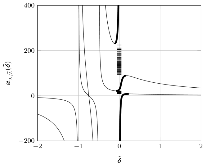
Figure 1. ${\boldsymbol{x}}_{\mathcal{I},\widetilde{\mathcal{I}}}({\boldsymbol{\tilde{\delta}}})$ for each component pairs $\mathcal{I}$ of $\mathcal{D}$ and $\widetilde{\mathcal{I}}$ of $\widetilde{\mathcal{D}}$. In thick line, positions for which $1-{\boldsymbol{x}}^{2}{\boldsymbol{\gamma}}({\boldsymbol{x}},{\boldsymbol{\tilde{\delta}}}){\boldsymbol{\tilde{\gamma}}}({\boldsymbol{x}},{\boldsymbol{\delta}})>0$. On the vertical axis, in black dashes, empirical eigenvalue positions for $N=1000$. Setting: $c=10$, $\nu=1/2(\delta_{1}+\delta_{2})$, $\tilde{\nu}=1/2(\delta_{1}+\delta_{10})$.

3.4. Properties of the graph of $\boldsymbol{x}$ versus $\boldsymbol{\tilde{\delta}}$ and the consequences

The two following propositions will help us bring out some of the properties of the graph of $\boldsymbol{x}$ versus $\boldsymbol{\tilde{\delta}}$. In their statements, we assume that the triples $(\boldsymbol{\tilde{\delta}}_{1},\boldsymbol{\delta}_{1},\boldsymbol{x}_{1})$ and $(\boldsymbol{\tilde{\delta}}_{2},\boldsymbol{\delta}_{2},\boldsymbol{x}_{2})$ satisfy both the statement of Proposition 3.2.

Lemma 3.5.

$\boldsymbol{\tilde{\delta}}_{1}\neq\boldsymbol{\tilde{\delta}}_{2}\Rightarrow\boldsymbol{x}_{1}\neq\boldsymbol{x}_{2}$ and $\boldsymbol{\delta}_{1}\neq\boldsymbol{\delta}_{2}\Rightarrow\boldsymbol{x}_{1}\neq\boldsymbol{x}_{2}$.

Proof.

We know that $\boldsymbol{\tilde{\delta}}_{i}=\lim_{z\in\mathbb{C}_{+}\to\boldsymbol{x}_{i}}\tilde{\delta}(z)$ for $i=1,2$. Assume that $\boldsymbol{\tilde{\delta}}_{1}\neq\boldsymbol{\tilde{\delta}}_{2}$. Then having $\boldsymbol{x}_{1}=\boldsymbol{x}_{2}$ would violate this convergence. ∎

Lemma 3.6.

If $\boldsymbol{\tilde{\delta}}_{1}<\boldsymbol{\tilde{\delta}}_{2}$, if $\boldsymbol{x}_{1}\boldsymbol{x}_{2}>0$, and if $[\boldsymbol{\delta}_{1}\wedge\boldsymbol{\delta}_{2},\boldsymbol{\delta}_{1}\vee\boldsymbol{\delta}_{2}]\subset{\mathcal{D}}$, then $\boldsymbol{x}_{1}<\boldsymbol{x}_{2}$.

Proof.

We use the identity

$$\Bigl{(}1-\boldsymbol{x}_{1}\boldsymbol{x}_{2}\gamma(\boldsymbol{x}_{1},\boldsymbol{x}_{2})\tilde{\gamma}(\boldsymbol{x}_{1},\boldsymbol{x}_{2})\Bigr{)}(\boldsymbol{\tilde{\delta}}_{1}-\boldsymbol{\tilde{\delta}}_{2})\\ =(\boldsymbol{x}_{1}-\boldsymbol{x}_{2})\int\frac{t}{\boldsymbol{x}_{1}\boldsymbol{x}_{2}(1+\boldsymbol{\delta}_{1}t)(1+\boldsymbol{\delta}_{2}t)}\,\tilde{\nu}(dt),$$

see (7). By the Cauchy-Schwarz inequality, $1-\boldsymbol{x}_{1}\boldsymbol{x}_{2}\gamma(\boldsymbol{x}_{1},\boldsymbol{x}_{2})\tilde{\gamma}(\boldsymbol{x}_{1},\boldsymbol{x}_{2})>0$. Let us show that the integral $I$ at the right hand side of the equation above is positive. Assume that for some $t\in\operatorname*{supp}(\tilde{\nu})$, the numbers $1+\boldsymbol{\delta}_{1}t$ and $1+\boldsymbol{\delta}_{2}t$ do not have the same sign. Then there exists $\boldsymbol{\delta}\in(\boldsymbol{\delta}_{1}\wedge\boldsymbol{\delta}_{2},\boldsymbol{\delta}_{1}\vee\boldsymbol{\delta}_{2})$ such that $1+\boldsymbol{\delta}t=0$. But this contradicts $[\boldsymbol{\delta}_{1}\wedge\boldsymbol{\delta}_{2},\boldsymbol{\delta}_{1}\vee\boldsymbol{\delta}_{2}]\subset{\mathcal{D}}$. Hence $I>0$, which shows that $\boldsymbol{x}_{1}-\boldsymbol{x}_{2}$ and $\boldsymbol{\tilde{\delta}}_{1}-\boldsymbol{\tilde{\delta}}_{2}$ have the same sign. ∎

In order to better understand the incidence of these propositions, let us describe more formally the procedure for determining the support of $\mu$. Equations (9) can be rewritten as $-\boldsymbol{x}\boldsymbol{\delta}\boldsymbol{\tilde{\delta}}=g(\boldsymbol{\tilde{\delta}})=\tilde{g}(\boldsymbol{\delta})$ where

$$g(\boldsymbol{\tilde{\delta}})=c\int\frac{\boldsymbol{\tilde{\delta}}t}{1+\boldsymbol{\tilde{\delta}}t}\nu(dt)\quad\text{and}\quad\tilde{g}(\boldsymbol{\delta})=\int\frac{\boldsymbol{\delta}t}{1+\boldsymbol{\delta}t}\tilde{\nu}(dt)$$

are both increasing on any interval of $\widetilde{\cal D}$ and $\cal D$ respectively. Let $\mathcal{I}$ and $\widetilde{\mathcal{I}}$ be two connected components of $\mathcal{D}$ and $\widetilde{\mathcal{D}}$ respectively. Assume that $\tilde{g}({\mathcal{I}})\cap g(\widetilde{\mathcal{I}})\neq\emptyset$. Since $\tilde{g}$ is increasing, it has a local inverse $\tilde{g}^{-1}_{\mathcal{I},\widetilde{\mathcal{I}}}$ on $g(\widetilde{\mathcal{I}})$. Let $\boldsymbol{\delta}=\tilde{g}^{-1}_{\mathcal{I},\widetilde{\mathcal{I}}}\circ g(\boldsymbol{\tilde{\delta}})$ and consider the function

$$\boldsymbol{x}_{\mathcal{I},\widetilde{\mathcal{I}}}(\boldsymbol{\tilde{\delta}})=-\frac{g(\boldsymbol{\tilde{\delta}})}{\boldsymbol{\delta}\boldsymbol{\tilde{\delta}}}=-\frac{g(\boldsymbol{\tilde{\delta}})}{\boldsymbol{\tilde{\delta}}\times\tilde{g}^{-1}_{\mathcal{I},\widetilde{\mathcal{I}}}\circ g(\boldsymbol{\tilde{\delta}})},$$ (13)

with domain the open set $\operatorname{dom}(\boldsymbol{x}_{{\cal I},\widetilde{\cal I}})=\{\boldsymbol{\tilde{\delta}}\in\widetilde{\cal I}\,:\,\exists\boldsymbol{\delta}\in{\cal I}\ \text{such that}\ \tilde{g}(\boldsymbol{\delta})=g(\boldsymbol{\tilde{\delta}})\ \text{and}\ \boldsymbol{\delta}\neq 0\}$. Computing $\boldsymbol{x}_{\mathcal{I},\widetilde{\mathcal{I}}}(\boldsymbol{\tilde{\delta}})$ on all connected components $\cal I$ and $\widetilde{\cal I}$ and dropping the values of $\boldsymbol{x}$ for which $1-\boldsymbol{x}^{2}\boldsymbol{\gamma}(\boldsymbol{x},\boldsymbol{\tilde{\delta}})\boldsymbol{\tilde{\gamma}}(\boldsymbol{x},\boldsymbol{\delta})>0$, we are of course left with $\operatorname*{supp}(\mu)\cap\mathbb{R}_{*}$.
Thanks to Lemmas 3.5-3.6, the functions $\boldsymbol{x}_{\mathcal{I},\widetilde{\mathcal{I}}}$ have the following properties:

1. For any $\boldsymbol{x}_{0}\in\mathbb{R}_{*}$, at most one function $\boldsymbol{x}_{\mathcal{I},\widetilde{\mathcal{I}}}$ satisfies $\boldsymbol{x}_{\mathcal{I},\widetilde{\mathcal{I}}}(\boldsymbol{\tilde{\delta}})=\boldsymbol{x}_{0}$ and $\boldsymbol{x}^{\prime}_{\mathcal{I},\widetilde{\mathcal{I}}}(\boldsymbol{\tilde{\delta}})>0$ by Lemma 3.5.
   Note that more than one function $\boldsymbol{x}_{\mathcal{I},\widetilde{\mathcal{I}}}$ can be possibly increasing at a given $\boldsymbol{\tilde{\delta}}\in\widetilde{\mathcal{D}}$, as the figure shows.

2. We show below that there is exactly one couple $({\cal I},\widetilde{\cal I})$ for which $\boldsymbol{x}_{\mathcal{I},\widetilde{\mathcal{I}}}$ has negative values and is increasing from $-\infty$ to zero where it is negative. Moreover, for any couple $({\cal I},\widetilde{\cal I})$ and for any $[\boldsymbol{\tilde{\delta}}_{1},\boldsymbol{\tilde{\delta}}_{2}]\in\widetilde{\mathcal{I}}$ such that $\boldsymbol{x}_{\mathcal{I},\widetilde{\mathcal{I}}}(\boldsymbol{\tilde{\delta}}_{i})>0$ and $\boldsymbol{x}^{\prime}_{\mathcal{I},\widetilde{\mathcal{I}}}(\boldsymbol{\tilde{\delta}}_{i})>0$, $i=1,2$, the function $\boldsymbol{x}_{\mathcal{I},\widetilde{\mathcal{I}}}(\tilde{\delta})$ never decreases between $\tilde{\delta}_{1}$ and $\tilde{\delta}_{2}$ by Lemma 3.6.
   In summary, if a branch of a $\boldsymbol{x}_{\mathcal{I},\widetilde{\mathcal{I}}}(\tilde{\delta})$ is increasing at two points $\tilde{\delta}_{1}$ and $\tilde{\delta}_{2}$, then it never decreases between these two points.

3. Let $b=\sup(\operatorname*{supp}(\nu))\in(0,\infty]$ and $\tilde{b}=\sup(\operatorname*{supp}(\tilde{\nu}))\in(0,\infty]$, and let us study the behavior of $\boldsymbol{x}_{\mathcal{I},\widetilde{\mathcal{I}}}$ when $\widetilde{\cal I}=(-b^{-1},\infty)$ and ${\cal I}=(-\tilde{b}^{-1},\infty)$. Assume $b=\tilde{b}=\infty$. By the fact that the functions $\delta(x)$ and $\tilde{\delta}(x)$ are both positive and increasing on $(-\infty,0)$ and by Lemma 3.5, the branch $\boldsymbol{x}_{\mathcal{I},\widetilde{\mathcal{I}}}(\boldsymbol{\tilde{\delta}})$ is increasing where it is negative, it is the only branch having this property, and $\boldsymbol{x}_{\mathcal{I},\widetilde{\mathcal{I}}}(\boldsymbol{\tilde{\delta}})\to-\infty$ as $\boldsymbol{\tilde{\delta}}\downarrow 0$.
   Assume now that $b=\infty$ and $\tilde{b}<\infty$. Here it is easy to notice that $g((-\tilde{b}^{-1},0))\cap\tilde{g}((0,\infty))=\emptyset$ which implies that we can replace ${\cal I}$ with $(0,\infty)$. As in the former case, the graph of $\boldsymbol{x}_{\mathcal{I},\widetilde{\mathcal{I}}}$ consists in one branch that has the same properties as regards the negative values of $\boldsymbol{x}$. The same conclusion holds when $b<\infty$ and $\tilde{b}=\infty$.
   Finally, assume that $b,\tilde{b}<\infty$. Here $g(\boldsymbol{\tilde{\delta}})/\boldsymbol{\tilde{\delta}}\approx C$ and $\boldsymbol{\delta}\approx C^{\prime}\boldsymbol{\tilde{\delta}}$ near zero, where $C,C^{\prime}>0$. Consequently, the graph of $\boldsymbol{x}_{\mathcal{I},\widetilde{\mathcal{I}}}(\boldsymbol{\tilde{\delta}})$ consists in two branches, one on $(-b^{-1},0)$ and one on $(0,\infty)$. The first branch converges to infinity as $\boldsymbol{\tilde{\delta}}\uparrow 0$, showing that $\mu$ is compactly supported, and the second branch behaves below zero as its analogues above. These two branches appear on the figure.

4. Assume that $a=\inf(\operatorname*{supp}(\nu)\cap\mathbb{R}_{*})>0$ and let $\widetilde{\cal I}=(-\infty,-a^{-1})$. Then $g(\boldsymbol{\tilde{\delta}})$ increases from $c$ as $\boldsymbol{\tilde{\delta}}$ increases from $-\infty$. If $\boldsymbol{\delta}<0$, then $\boldsymbol{x}_{\mathcal{I},\widetilde{\mathcal{I}}}(\boldsymbol{\tilde{\delta}})<0$ since $g(\boldsymbol{\tilde{\delta}})/\boldsymbol{\tilde{\delta}}<0$, and the conclusions of Item (3) show that the branches $\boldsymbol{x}_{\mathcal{I},\widetilde{\mathcal{I}}}$ need not be considered for determining $\operatorname*{supp}(\mu)$ when ${\cal I}\subset(-\infty,0)$. It remains to study $\boldsymbol{x}_{\mathcal{I},\widetilde{\mathcal{I}}}$ for ${\cal I}=(-\tilde{b}^{-1},\infty)$. On $(0,\infty)$, the function $\tilde{g}(\boldsymbol{\delta})$ increases from $0$ to $1$, hence $\tilde{g}((0,\infty))\cap g(\widetilde{\cal I})\neq\emptyset$ if and only if $c<1$. In that case, it can be checked that $\boldsymbol{x}_{\mathcal{I},\widetilde{\mathcal{I}}}(\boldsymbol{\tilde{\delta}})$ increases from $0$ as $\boldsymbol{\tilde{\delta}}$ increases from $-\infty$. In conclusion, if $a>0$ and $c<1$, then $\inf(\operatorname*{supp}(\mu)\cap\mathbb{R}_{*})>0$, and the location of this infimum is provided by the branch $\boldsymbol{x}_{\mathcal{I},\widetilde{\mathcal{I}}}$.
   Similarly, if $\tilde{a}=\inf(\operatorname*{supp}(\tilde{\nu})\cap\mathbb{R}_{*})>0$, ${\cal I}=(-\infty,-\tilde{a}^{-1})$ and $\widetilde{\cal I}\subset(-\infty,0)$, then the branches $\boldsymbol{x}_{\mathcal{I},\widetilde{\mathcal{I}}}$ need not be considered. If in addition $c>1$, then $\inf(\operatorname*{supp}(\mu)\cap\mathbb{R}_{*})>0$, and the location of this infimum is provided by the branch $\boldsymbol{x}_{\mathcal{I},\widetilde{\mathcal{I}}}$ for ${\cal I}=(-\infty,-\tilde{a}^{-1})$ and $\widetilde{\cal I}=(-b^{-1},\infty)$.

We terminate this paragraph with the following two results:

Proposition 3.3.

Assume that $\operatorname*{supp}(\nu)\cap\mathbb{R}_{*}$ and $\operatorname*{supp}(\tilde{\nu})\cap\mathbb{R}_{*}$ consist in $K$ and $\widetilde{K}$ connected components respectively. Then $\operatorname*{supp}(\mu)\cap\mathbb{R}_{*}$ consists in at most $K\widetilde{K}$ connected components.

Proof.

When $\nu$ is compactly supported, $\operatorname*{supp}(\nu-\nu(\{0\})\boldsymbol{d}_{0})=[a_{1},b_{1}]\cup[a_{2},b_{2}]\cup\cdots\cup[a_{K},b_{K}]$ where $0<a_{1}\leq b_{1}<a_{2}\leq b_{2}<\cdots<a_{K}\leq b_{K}<\infty$ or $0=a_{1}<b_{1}<a_{2}\leq b_{2}<\cdots<a_{K}\leq b_{K}<\infty$. In the first case, the connected components of $\widetilde{\cal D}$ are $\widetilde{\cal I}_{0}=(-\infty,-a_{1}^{-1})$, $\widetilde{\cal I}_{1}=(-b_{1}^{-1},-a_{2}^{-1}),\ldots,\widetilde{\cal I}_{K}=(-b_{K}^{-1},\infty)$. In the second case, these connected components are $\widetilde{\cal I}_{1},\ldots,\widetilde{\cal I}_{K}$. If $\nu$ is not compactly supported, $a_{K}<b_{K}=\infty$ and the expressions of the connected components of $\widetilde{\cal D}$ are unchanged. With similar notations, the connected components of $\cal D$ are ${\cal I}_{0},\ldots,{\cal I}_{\widetilde{K}}$ or ${\cal I}_{1},\ldots,{\cal I}_{\widetilde{K}}$ according to whether $\inf(\operatorname*{supp}(\tilde{\nu})\cap\mathbb{R}_{*})$ is positive or not. Let $s=\inf(\operatorname*{supp}(\mu)\cap\mathbb{R}_{*})$ and $S=\sup(\operatorname*{supp}(\mu))$. Following the observations we just made, we notice that the only possible $\boldsymbol{x}_{{\cal I}_{k},\widetilde{\cal I}_{\tilde{k}}}(\boldsymbol{\tilde{\delta}})\in(s,S)$ such that $\boldsymbol{x}_{{\cal I}_{k},\widetilde{\cal I}_{\tilde{k}}}^{\prime}(\boldsymbol{\tilde{\delta}})>0$ are those for which $1\leq k\leq K$, $1\leq\tilde{k}\leq\widetilde{K}$, and $(k,\tilde{k})\neq(K,\widetilde{K})$. Therefore, the number of intervals of $\operatorname*{supp}(\mu)^{c}\cap(s,S)$ is upper bounded by $K\widetilde{K}-1$, hence the result. ∎

Proposition 3.4.

$\operatorname*{supp}(\mu)$ is compact if and only if $\operatorname*{supp}(\nu)$ and $\operatorname*{supp}(\tilde{\nu})$ are compact.

Proof.

The “if” part has been shown by Item (3) above. Assume $\operatorname*{supp}(\mu)$ is compact. The fact that $\operatorname*{supp}(\rho)\cap\mathbb{R}_{*}=\operatorname*{supp}(\tilde{\rho})\cap\mathbb{R}_{*}=\operatorname*{supp}(\mu)\cap\mathbb{R}_{*}$ and the equation $m_{\tilde{\nu}}(-\delta(z)^{-1})=\delta(z)+z\delta^{2}(z)\tilde{\delta}(z)$ show that $m_{\tilde{\nu}}(z)$ can be analytically extended to $(A,\infty)$ for $A$ large enough, hence the compactness of $\operatorname*{supp}(\tilde{\nu})$. A similar conclusion holds for $\operatorname*{supp}(\nu)$. ∎

3.5. Properties of the density of $\mu$ on $\mathbb{R}_{*}$

Theorem 3.2.

The density $f(x)$ specified in the statement of Theorem 3.1 is analytic for every $x\neq 0$ for which $f(x)>0$.

Proof.

We can assume that $\nu$ is not a Dirac measure, otherwise see [20]. Let $x_{0}\neq 0$ be such that $f(x_{0})>0$. We start by showing that $\tilde{\delta}(z)$ can be analytically extended from $\mathbb{C}_{+}$ to a neighborhood of $x_{0}$ in $\mathbb{C}$. Write

$$\gamma(x_{0},x_{0})=\lim_{z\in\mathbb{C}_{+}\to x_{0}}\gamma(z,z),\quad\tilde{\gamma}(x_{0},x_{0})=\lim_{z\in\mathbb{C}_{+}\to x_{0}}\tilde{\gamma}(z,z),$$

$$\Gamma(x_{0},x_{0})=\lim_{z\in\mathbb{C}_{+}\to x_{0}}\gamma(z,z^{*}),\quad\widetilde{\Gamma}(x_{0},x_{0})=\lim_{z\in\mathbb{C}_{+}\to x_{0}}\tilde{\gamma}(z,z^{*}).$$

Making $z\in\mathbb{C}_{+}$ converge to $x_{0}$ in Equation (8) and recalling that the integral at the right hand side of this equation remains bounded and that $\Im\tilde{\delta}(x_{0})>0$, we get that $x_{0}^{2}\Gamma(x_{0},x_{0})\widetilde{\Gamma}(x_{0},x_{0})=1$. Any integrable random variable $X$ satisfies $|\mathbb{E}X|\leq\mathbb{E}|X|$, the equality being achieved if and only if $X=\theta|X|$ almost everywhere, where $\theta$ is a modulus one constant. Consequently, $|\gamma(x_{0},x_{0})|<\Gamma(x_{0},x_{0})$ since $\nu$ is not a Dirac measure, and $|\tilde{\gamma}(x_{0},x_{0})|\leq\widetilde{\Gamma}(x_{0},x_{0})$. Therefore, $|x_{0}^{2}\gamma(x_{0},x_{0})\tilde{\gamma}(x_{0},x_{0})|<1$. Now, since $\Im\tilde{\delta}(x_{0})>0$, it is easy to see by inspecting Equation (4) that the function $F(\tilde{\delta},z)$ which is holomorphic on $\mathbb{C}_{+}^{2}$ can be analytically extended to a neighborhood of $(\tilde{\delta}(x_{0}),x_{0})$ in $\mathbb{C}_{+}\times\mathbb{C}_{*}$ where $\mathbb{C}_{*}=\mathbb{C}-\{0\}$. Observing that

$$\frac{\partial F}{\partial\tilde{\delta}}(\tilde{\delta}(x_{0}),x_{0})=-1+x_{0}^{2}\gamma(x_{0},x_{0})\tilde{\gamma}(x_{0},x_{0})\neq 0$$

and invoking the holomorphic implicit function theorem, we get that there exists a neighborhood $V\subset\mathbb{C}_{*}$ of $x_{0}$, a neighborhood $V^{\prime}\subset\mathbb{C}_{+}$ of $\tilde{\delta}(x_{0})$ and a holomorphic function $\underline{\tilde{\delta}}:V\to V^{\prime}$ such that

$$\{(z,\tilde{\delta})\in V\times V^{\prime}\,:\,F(\tilde{\delta},z)=0\}\ =\ \{(z,\underline{\tilde{\delta}}(z))\,:\,z\in V\}.$$

Since $\tilde{\delta}(z)$ and $\underline{\tilde{\delta}}(z)$ coincide on $V\cap\mathbb{C}_{+}$, the function $\underline{\tilde{\delta}}(z)$ is an analytic extension of $\tilde{\delta}(z)$ on $V$.
This result shows in conjunction with Equation (3) that $m(z)$ can be extended analytically to $V$. Therefore, writing $m(z)=\sum_{\ell\geq 0}a_{\ell}(z-x_{0})^{\ell}$ we get that $f(x)=\pi^{-1}\sum_{\ell\geq 0}\Im a_{\ell}\,(x-x_{0})^{\ell}$ near $x_{0}$. ∎

We now study the behavior of the density $f(x)$ near a boundary point $a>0$ of $\operatorname*{supp}(\mu)$. The observations made above show that when $a$ is a left end point (resp. a right end point) of $\operatorname*{supp}(\mu)$, it is a local supremum (resp. a local infimum) of one of the functions $\boldsymbol{x}_{{\cal I},\widetilde{\cal I}}$. Parallelling the assumptions made in [15], [20] and [5], we restrict ourselves to the case where $a=\boldsymbol{x}_{{\cal I},\widetilde{\cal I}}(\boldsymbol{\tilde{\delta}}_{a})$ for some $\boldsymbol{\tilde{\delta}}_{a}\in\operatorname{dom}(\boldsymbol{x}_{{\cal I},\widetilde{\cal I}})$. In that case, $\boldsymbol{x}_{{\cal I},\widetilde{\cal I}}$ is of course analytical around $\boldsymbol{\tilde{\delta}}_{a}$ and $\boldsymbol{x}_{{\cal I},\widetilde{\cal I}}^{\prime}(\boldsymbol{\tilde{\delta}}_{a})=0$.
Note that this assumption might not be satisfied for some choices of the measures $\nu$ and $\tilde{\nu}$. Assuming $a>0$ is a left end point of $\operatorname*{supp}(\mu)$, it is for instance possible that the function $\boldsymbol{x}_{{\cal I},\widetilde{\cal I}}(\boldsymbol{\tilde{\delta}})$ increases to $a$ as $\boldsymbol{\tilde{\delta}}\uparrow\boldsymbol{\tilde{\delta}}_{a}$ with $-\boldsymbol{\tilde{\delta}}_{a}^{-1}\in\partial\nu$. We however note that our assumption is valid when the measures $\nu$ and $\tilde{\nu}$ are both discrete.

Theorem 3.3.

Let $\cal I$ and $\widetilde{\cal I}$ be two connected components of $\cal D$ and $\widetilde{\cal D}$ respectively, and assume that $\boldsymbol{x}_{{\cal I},\widetilde{\cal I}}$ reaches a maximum at a point $\boldsymbol{\tilde{\delta}}_{a}\in\operatorname{dom}(\boldsymbol{x}_{{\cal I},\widetilde{\cal I}})$. Then $\boldsymbol{x}_{{\cal I},\widetilde{\cal I}}^{\prime\prime}(\boldsymbol{\tilde{\delta}}_{a})<0$. Furthermore, for $\varepsilon>0$ small enough, $f(x)=H(\sqrt{x-a})$ on $(a,a+\varepsilon)$ where $H(x)$ is a real analytical function near zero, $H(0)=0$, and

$$H^{\prime}(0)=\frac{1}{\pi a}\sqrt{\frac{-2}{\boldsymbol{x}_{{\cal I},\widetilde{\cal I}}^{\prime\prime}(\boldsymbol{\tilde{\delta}}_{a})}}\int\frac{t}{(1+\boldsymbol{\tilde{\delta}}_{a}t)^{2}}\nu(dt).$$

Assume now that $\boldsymbol{x}_{{\cal I},\widetilde{\cal I}}$ reaches a minimum at a point $\boldsymbol{\tilde{\delta}}_{a}\in\operatorname{dom}(\boldsymbol{x}_{{\cal I},\widetilde{\cal I}})$. Then $\boldsymbol{x}_{{\cal I},\widetilde{\cal I}}^{\prime\prime}(\boldsymbol{\tilde{\delta}}_{a})>0$. Furthermore, for $\varepsilon>0$ small enough, $f(x)=H(\sqrt{a-x})$ on $(a-\varepsilon,a)$ where $H(x)$ is a real analytical function near zero, $H(0)=0$, and

$$H^{\prime}(0)=\frac{1}{\pi a}\sqrt{\frac{2}{\boldsymbol{x}_{{\cal I},\widetilde{\cal I}}^{\prime\prime}(\boldsymbol{\tilde{\delta}}_{a})}}\int\frac{t}{(1+\boldsymbol{\tilde{\delta}}_{a}t)^{2}}\nu(dt).$$

To prove the theorem, we start with the following lemma which is proven in the appendix:

Lemma 3.7.

Assume that either $\nu$ or $\tilde{\nu}$ is not a Dirac measure. Let $({\boldsymbol{\tilde{\delta}}}_{a},a)$ with ${a}\neq 0$ satisfy

$$\boldsymbol{F}({\boldsymbol{\tilde{\delta}}}_{a},{a})=0,\quad\frac{\partial\boldsymbol{F}}{\partial{\boldsymbol{\tilde{\delta}}}}({\boldsymbol{\tilde{\delta}}}_{a},{a})=0$$

where the function $\boldsymbol{F}(\boldsymbol{\tilde{\delta}},\boldsymbol{x})$ is defined by Equation (11). Then

$$\frac{\partial^{2}\boldsymbol{F}}{\partial{\boldsymbol{\tilde{\delta}}}^{2}}({\boldsymbol{\tilde{\delta}}}_{a},{a})=0\leavevmode\nobreak\ \Rightarrow\leavevmode\nobreak\ \frac{\partial^{3}\boldsymbol{F}}{\partial{\boldsymbol{\tilde{\delta}}}^{3}}({\boldsymbol{\tilde{\delta}}}_{a},{a})\neq 0.$$

Proof of Theorem 3.3.

We follow the argument of [15]. We first assume that $\boldsymbol{x}_{{\cal I},\widetilde{\cal I}}$ reaches a maximum at $\boldsymbol{\tilde{\delta}}_{a}\in\widetilde{\cal I}$ and prove that $\boldsymbol{x}_{{\cal I},\widetilde{\cal I}}^{\prime\prime}(\boldsymbol{\tilde{\delta}}_{a})<0$. Observe that $\boldsymbol{x}_{{\cal I},\widetilde{\cal I}}(\boldsymbol{\tilde{\delta}})$ satisfies $\boldsymbol{F}(\boldsymbol{\tilde{\delta}},\boldsymbol{x}_{{\cal I},\widetilde{\cal I}}(\boldsymbol{\tilde{\delta}}))=0$, and that $\partial\boldsymbol{F}/\partial\boldsymbol{x}=\int t(\boldsymbol{x}(1+\boldsymbol{\delta}t))^{-2}\tilde{\nu}(dt)>0$. By the chain rule for differentiation,

$$0 =\frac{\partial\boldsymbol{F}}{\partial\boldsymbol{\tilde{\delta}}}+\frac{\partial\boldsymbol{F}}{\partial\boldsymbol{x}}\boldsymbol{x}_{{\cal I},\widetilde{\cal I}}^{\prime}(\boldsymbol{\tilde{\delta}}),$$

$$0 =\frac{\partial^{2}\boldsymbol{F}}{\partial\boldsymbol{\tilde{\delta}}^{2}}+\left(\frac{\partial^{2}\boldsymbol{F}}{\partial\boldsymbol{x}^{2}}+2\frac{\partial^{2}\boldsymbol{F}}{\partial\boldsymbol{\tilde{\delta}}\partial\boldsymbol{x}}\right)\boldsymbol{x}_{{\cal I},\widetilde{\cal I}}^{\prime}(\boldsymbol{\tilde{\delta}})+\frac{\partial\boldsymbol{F}}{\partial\boldsymbol{x}}\boldsymbol{x}_{{\cal I},\widetilde{\cal I}}^{\prime\prime}(\boldsymbol{\tilde{\delta}}).$$

If we assume that $\boldsymbol{x}_{{\cal I},\widetilde{\cal I}}^{\prime\prime}(\boldsymbol{\tilde{\delta}}_{a})=0$, then $(\partial^{2}\boldsymbol{F}/\partial\boldsymbol{\tilde{\delta}}^{2})(\boldsymbol{\tilde{\delta}}_{a},a)=0$ and it is furthermore easy to check that

$$\boldsymbol{x}^{(3)}(\boldsymbol{\tilde{\delta}}_{a})=-\frac{\partial^{3}\boldsymbol{F}/\partial\boldsymbol{\tilde{\delta}}^{3}}{\partial\boldsymbol{F}/\partial\boldsymbol{x}}(\boldsymbol{\tilde{\delta}}_{a},a).$$

By Lemma 3.7, $\boldsymbol{x}^{(3)}(\boldsymbol{\tilde{\delta}}_{a})\neq 0$, but this contradicts the fact that the first non zero derivative of a function at a local extremum is of even order. Hence $\boldsymbol{x}_{{\cal I},\widetilde{\cal I}}^{\prime\prime}(\boldsymbol{\tilde{\delta}}_{a})<0$.
Equation (13) shows that $\boldsymbol{x}_{{\cal I},\widetilde{\cal I}}$ can be analytically extended to a function $z_{{\cal I},\widetilde{\cal I}}$ in a neighborhood of $\boldsymbol{\tilde{\delta}}_{a}$ in the complex plane. Since $\boldsymbol{x}_{{\cal I},\widetilde{\cal I}}^{\prime}(\boldsymbol{\tilde{\delta}}_{a})=0$ and $\boldsymbol{x}_{{\cal I},\widetilde{\cal I}}^{\prime\prime}(\boldsymbol{\tilde{\delta}}_{a})<0$, we can write $z_{{\cal I},\widetilde{\cal I}}(\tilde{\delta})-a=\varphi(\tilde{\delta})^{2}$ in this neighborhood where $\varphi$ is an analytical function satisfying $\varphi(\boldsymbol{\tilde{\delta}}_{a})=0$ and $(\varphi^{\prime}(\boldsymbol{\tilde{\delta}}_{a}))^{2}=\boldsymbol{x}_{{\cal I},\widetilde{\cal I}}^{\prime\prime}(\boldsymbol{\tilde{\delta}}_{a})/2$. We choose $\varphi$ such that $\varphi^{\prime}(\boldsymbol{\tilde{\delta}}_{a})=-\imath(-\boldsymbol{x}_{{\cal I},\widetilde{\cal I}}^{\prime\prime}(\boldsymbol{\tilde{\delta}}_{a})/2)^{1/2}$. If we choose $x>a$ such that $x-a$ is small enough, then $z_{{\cal I},\widetilde{\cal I}}(\tilde{\delta}(x))-a=\varphi(\tilde{\delta}(x))^{2}$, and moreover $z_{{\cal I},\widetilde{\cal I}}(\tilde{\delta}(x))=x$. Considering the local inverse $\Phi$ of $\varphi$ in a neighborhood of $\boldsymbol{\tilde{\delta}}_{a}$, we get that $\tilde{\delta}(x)=\Phi(\sqrt{x-a})$ where the analytic function $\Phi$ satisfies $\Phi(0)=\boldsymbol{\tilde{\delta}}_{a}$ and $\Phi^{\prime}(0)=1/\varphi^{\prime}(\boldsymbol{\tilde{\delta}}_{a})=\imath(-2/\boldsymbol{x}_{{\cal I},\widetilde{\cal I}}^{\prime\prime}(\boldsymbol{\tilde{\delta}}_{a}))^{1/2}$ (thus the choice of $\varphi^{\prime}(\boldsymbol{\tilde{\delta}}_{a})$ ensures that $\Im\tilde{\delta}(x)>0$). Using the equation $\Im m(x)=-x^{-1}\int\Im((1+\tilde{\delta}(x)t)^{-1})\nu(dt)$, we get the result. The case where $\boldsymbol{x}_{{\cal I},\widetilde{\cal I}}$ reaches a minimum at $\boldsymbol{\tilde{\delta}}_{a}$ is treated similarly. ∎

Appendix A Proof of Lemma 3.7

First recall that

$$\frac{\partial\boldsymbol{F}}{\partial{\boldsymbol{\tilde{\delta}}}}({\boldsymbol{\tilde{\delta}}},{\boldsymbol{x}})={\boldsymbol{x}}^{2}{\boldsymbol{\gamma}}({\boldsymbol{x}},{\boldsymbol{\tilde{\delta}}})\boldsymbol{\tilde{\gamma}}({\boldsymbol{x}},{\boldsymbol{\delta}})-1$$ (14)

so that ${a}^{2}{\boldsymbol{\gamma}}_{a}\boldsymbol{\tilde{\gamma}}_{a}=1$, with ${\boldsymbol{\gamma}}_{a}={\boldsymbol{\gamma}}({a},{\boldsymbol{\tilde{\delta}}}_{a})$, $\boldsymbol{\tilde{\gamma}}_{a}=\boldsymbol{\tilde{\gamma}}({a},{\boldsymbol{\delta}}_{a})$, and

$${\boldsymbol{\delta}}_{a}=c\int\frac{t}{-{a}(1+{\boldsymbol{\tilde{\delta}}}_{a}t)}\nu(dt).$$

Differentiating (14), the equation $(\partial^{2}\boldsymbol{F}/\partial{\boldsymbol{\tilde{\delta}}}^{2})({\boldsymbol{\tilde{\delta}}}_{a},{a})=0$ reads

$$\boldsymbol{\tilde{\gamma}}_{a}c\int\frac{t^{3}}{(1+{\boldsymbol{\tilde{\delta}}}_{a}t)^{3}}\nu(dt)+{a}{\boldsymbol{\gamma}}_{a}^{2}\int\frac{t^{3}}{(1+{\boldsymbol{\delta}}_{a}t)^{3}}\tilde{\nu}(dt)=0$$ (15)

where we used

$$\frac{\partial}{\partial{\boldsymbol{\tilde{\delta}}}}\left(c\int\frac{t}{-{\boldsymbol{x}}(1+{\boldsymbol{\tilde{\delta}}}t)}\nu(dt)\right)({\boldsymbol{\tilde{\delta}}}_{a},{a})={a}{\boldsymbol{\gamma}}_{a}.$$

Assume now that $(\partial^{3}\boldsymbol{F}/\partial{\boldsymbol{\tilde{\delta}}}^{3})({\boldsymbol{\tilde{\delta}}}_{a},{a})=0$. A second differentiation of (14) leads then to

$$0 =2\frac{{\boldsymbol{\gamma}}_{a}}{a}c\int\frac{t^{3}}{(1+{\boldsymbol{\delta}}_{a}t)^{3}}\tilde{\nu}(dt)\int\frac{t^{3}}{(1+{\boldsymbol{\tilde{\delta}}}_{a}t)^{3}}\nu(dt)$$

$$+\boldsymbol{\tilde{\gamma}}_{a}c\int\frac{t^{4}}{(1+{\boldsymbol{\tilde{\delta}}}_{a}t)^{4}}\nu(dt)+{a}^{2}{\boldsymbol{\gamma}}_{a}^{3}\int\frac{t^{4}}{(1+{\boldsymbol{\delta}}_{a}t)^{4}}\tilde{\nu}(dt).$$

Using ${a}^{2}{\boldsymbol{\gamma}}_{a}\boldsymbol{\tilde{\gamma}}_{a}=1$, replace now ${\boldsymbol{\gamma}}_{a}/{a}$ by $1/({a}^{3}\boldsymbol{\tilde{\gamma}}_{a})$ in the leftmost term and ${a}^{2}{\boldsymbol{\gamma}}_{a}^{3}$ by ${\boldsymbol{\gamma}}_{a}^{2}/\boldsymbol{\tilde{\gamma}}_{a}$ in the rightmost term. Multiplying the result by $\boldsymbol{\tilde{\gamma}}_{a}$ leads to

$$0 =2\frac{c}{{a}^{3}}\int\frac{t^{3}}{(1+{\boldsymbol{\delta}}_{a}t)^{3}}\tilde{\nu}(dt)\int\frac{t^{3}}{(1+{\boldsymbol{\tilde{\delta}}}_{a}t)^{3}}\nu(dt)$$

$$+\boldsymbol{\tilde{\gamma}}_{a}^{2}c\int\frac{t^{4}}{(1+{\boldsymbol{\tilde{\delta}}}_{a}t)^{4}}\nu(dt)+{\boldsymbol{\gamma}}_{a}^{2}\int\frac{t^{4}}{(1+{\boldsymbol{\delta}}_{a}t)^{4}}\tilde{\nu}(dt).$$ (16)

We now use (15) and ${a}^{2}{\boldsymbol{\gamma}}_{a}\boldsymbol{\tilde{\gamma}}_{a}=1$ to write the two equations:

$$2\frac{c}{{a}^{3}}\int\frac{t^{3}}{(1+{\boldsymbol{\tilde{\delta}}}_{a}t)^{3}}\nu(dt) =-\frac{2}{{a}^{2}}\frac{\boldsymbol{\gamma}_{a}^{2}}{\boldsymbol{\tilde{\gamma}}_{a}}\int\frac{t^{3}}{(1+\boldsymbol{\delta}_{a}t)^{3}}\tilde{\nu}(dt)$$

$$2\frac{c}{{a}^{3}}\int\frac{t^{3}}{(1+{\boldsymbol{\delta}}_{a}t)^{3}}\tilde{\nu}(dt) =-\frac{2c^{2}}{{a}^{2}}\frac{\boldsymbol{\tilde{\gamma}}_{a}^{2}}{{\boldsymbol{\gamma}}_{a}}\int\frac{t^{3}}{(1+{\boldsymbol{\tilde{\delta}}}_{a}t)^{3}}\nu(dt).$$

Replacing the corresponding terms in the leftmost term of (A) leads to the two equations

$$\frac{2}{{a}^{2}}\frac{{\boldsymbol{\gamma}}_{a}^{2}}{\boldsymbol{\tilde{\gamma}}_{a}}\left(\int\frac{t^{3}}{(1+{\boldsymbol{\delta}}_{a}t)^{3}}\tilde{\nu}(dt)\right)^{2}-\boldsymbol{\tilde{\gamma}}_{a}^{2}c\int\frac{t^{4}}{(1+{\boldsymbol{\tilde{\delta}}}_{a}t)^{4}}\nu(dt)-{\boldsymbol{\gamma}}_{a}^{2}\int\frac{t^{4}}{(1+{\boldsymbol{\delta}}_{a}t)^{4}}\tilde{\nu}(dt) =0$$

$$\frac{2}{{a}^{2}}\frac{\boldsymbol{\tilde{\gamma}}_{a}^{2}}{{\boldsymbol{\gamma}}_{a}}\left(c\int\frac{t^{3}}{(1+{\boldsymbol{\tilde{\delta}}}_{a}t)^{3}}\nu(dt)\right)^{2}-\boldsymbol{\tilde{\gamma}}_{a}^{2}c\int\frac{t^{4}}{(1+{\boldsymbol{\tilde{\delta}}}_{a}t)^{4}}\nu(dt)-{\boldsymbol{\gamma}}_{a}^{2}\int\frac{t^{4}}{(1+{\boldsymbol{\delta}}_{a}t)^{4}}\tilde{\nu}(dt) =0.$$

Multiplying each equation by ${\boldsymbol{\gamma}}_{a}\boldsymbol{\tilde{\gamma}}_{a}$ and averaging then gives:

$$0 =\frac{1}{{a}^{2}}{\boldsymbol{\gamma}}_{a}^{3}\left(\int\frac{t^{3}}{(1+{\boldsymbol{\delta}}_{a}t)^{3}}\tilde{\nu}(dt)\right)^{2}+\frac{1}{{a}^{2}}\boldsymbol{\tilde{\gamma}}_{a}^{3}\left(c\int\frac{t^{3}}{(1+{\boldsymbol{\tilde{\delta}}}_{a}t)^{3}}\nu(dt)\right)^{2}$$

$$-\boldsymbol{\tilde{\gamma}}_{a}^{3}{\boldsymbol{\gamma}}_{a}c\int\frac{t^{4}}{(1+{\boldsymbol{\tilde{\delta}}}_{a}t)^{4}}\nu(dt)-{\boldsymbol{\gamma}}_{a}^{3}\boldsymbol{\tilde{\gamma}}_{a}\int\frac{t^{4}}{(1+{\boldsymbol{\delta}}_{a}t)^{4}}\tilde{\nu}(dt).$$ (17)

Remark now, by expanding the definition of ${\tilde{\gamma}}_{a}$ that

$$\frac{1}{{a}^{2}}{\boldsymbol{\gamma}}_{a}^{3}\left(\int\frac{t^{3}}{(1+{\boldsymbol{\delta}}_{a}t)^{3}}\tilde{\nu}(dt)\right)^{2}-{\boldsymbol{\gamma}}_{a}^{3}\boldsymbol{\tilde{\gamma}}_{a}\int\frac{t^{4}}{(1+{\boldsymbol{\delta}}_{a}t)^{4}}\tilde{\nu}(dt)$$

$$=\frac{{\boldsymbol{\gamma}}_{a}^{3}}{{a}^{2}}\left[\left(\int\frac{t^{3}}{(1+{\boldsymbol{\delta}}_{a}t)^{3}}\tilde{\nu}(dt)\right)^{2}-\int\frac{t^{2}}{(1+{\boldsymbol{\delta}}_{a}t)^{2}}\tilde{\nu}(dt)\int\frac{t^{4}}{(1+{\boldsymbol{\delta}}_{a}t)^{4}}\tilde{\nu}(dt)\right]$$

$$\leq 0$$

with the inequality arising from Cauchy–Schwarz. The case of equality holds only if $\tilde{\nu}$ is a Dirac measure. Similarly,

$$\frac{1}{{a}^{2}}\boldsymbol{\tilde{\gamma}}_{a}^{3}\left(c\int\frac{t^{3}}{(1+{\boldsymbol{\tilde{\delta}}}_{a}t)^{3}}\nu(dt)\right)^{2}-\boldsymbol{\tilde{\gamma}}_{a}^{3}{\boldsymbol{\gamma}}_{a}c\int\frac{t^{4}}{(1+{\boldsymbol{\tilde{\delta}}}_{a}t)^{4}}\nu(dt)$$

$$=\frac{\boldsymbol{\tilde{\gamma}}_{a}^{3}}{{a}^{2}}\left[\left(c\int\frac{t^{3}}{(1+{\boldsymbol{\tilde{\delta}}}_{a}t)^{3}}\nu(dt)\right)^{2}-\left(c\int\frac{t^{2}}{(1+{\boldsymbol{\tilde{\delta}}}_{a}t)^{2}}\nu(dt)\right)\left(c\int\frac{t^{4}}{(1+{\boldsymbol{\tilde{\delta}}}_{a}t)^{4}}\nu(dt)\right)\right]$$

$$\leq 0$$

with equality only if $\nu$ is a Dirac measure. Therefore, to ensure (A), both $\nu$ and $\tilde{\nu}$ must be Dirac measures, which goes against the hypothesis.

References

- [1] Z. D. Bai and J. W. Silverstein. No eigenvalues outside the support of the limiting spectral distribution of large-dimensional sample covariance matrices. Ann. Probab., 26(1):316–345, 1998.
- [2] Z. D. Bai and J. W. Silverstein. Exact separation of eigenvalues of large-dimensional sample covariance matrices. Ann. Probab., 27(3):1536–1555, 1999.
- [3] Z. D. Bai and J. W. Silverstein. No eigenvalues outside the support of the limiting spectral distribution of information-plus-noise type matrices. Random Matrices: Theory and Applications, 1(1), 2012.
- [4] A. Boutet de Monvel, A. Khorunzhy, and V. Vasilchuk. Limiting eigenvalue distribution of random matrices with correlated entries. Markov Process. Related Fields, 2(4):607–636, 1996.
- [5] R. Brent Dozier and J. W. Silverstein. Analysis of the limiting spectral distribution of large dimensional information-plus-noise type matrices. J. Multivariate Anal., 98(6):1099–1122, 2007.
- [6] N. El Karoui. Tracy-Widom limit for the largest eigenvalue of a large class of complex sample covariance matrices. Ann. Probab., 35(2):663–714, 2007.
- [7] K. Fritzsche and H. Grauert. From holomorphic functions to complex manifolds, volume 213 of Graduate Texts in Mathematics. Springer-Verlag, New York, 2002.
- [8] V. L. Girko. Theory of random determinants, volume 45 of Mathematics and its Applications (Soviet Series). Kluwer Academic Publishers Group, Dordrecht, 1990. Translated from the Russian.
- [9] V. L. Girko. Theory of stochastic canonical equations. Vol. I and II, volume 535 of Mathematics and its Applications. Kluwer Academic Publishers, Dordrecht, 2001.
- [10] W. Hachem, P. Loubaton, X. Mestre, J. Najim, and P. Vallet. Large information plus noise random matrix models and consistent subspace estimation in large sensor networks. Random Matrices: Theory and Applications, 01(02):1150006, 2012.
- [11] W. Hachem, P. Loubaton, and J. Najim. The empirical distribution of the eigenvalues of a Gram matrix with a given variance profile. Ann. Inst. H. Poincaré Probab. Statist., 42(6):649–670, 2006.
- [12] W. Hachem, Ph. Loubaton, and J. Najim. Deterministic equivalents for certain functionals of large random matrices. Ann. Appl. Probab., 17(3):875–930, 2007.
- [13] M.G. Krein and A.A. Nudelman. The Markov Moment Problem and Extremal Problems. American Mathematical Society, Providence, Rhode Island, 1997.
- [14] P. Loubaton and P. Vallet. Almost sure localization of the eigenvalues in a gaussian information plus noise model–application to the spiked models. Electronic Journal of Probability, 16:1934–1959, 2011.
- [15] V. A. Marčenko and L. A. Pastur. Distribution of eigenvalues in certain sets of random matrices. Mat. Sb. (N.S.), 72 (114):507–536, 1967.
- [16] X. Mestre. Improved estimation of eigenvalues and eigenvectors of covariance matrices using their sample estimates. IEEE Trans. Inform. Theory, 54(11):5113–5129, 2008.
- [17] X. Mestre. On the asymptotic behavior of the sample estimates of eigenvalues and eigenvectors of covariance matrices. IEEE Trans. Signal Process., 56(11):5353–5368, 2008.
- [18] D. Paul and J. W. Silverstein. No eigenvalues outside the support of the limiting empirical spectral distribution of a separable covariance matrix. Journal of Multivariate Analysis, 100(1):37 – 57, 2009.
- [19] D. Shlyakhtenko. Random Gaussian band matrices and freeness with amalgamation. Internat. Math. Res. Notices, (20):1013–1025, 1996.
- [20] J. W. Silverstein and S.-I. Choi. Analysis of the limiting spectral distribution of large-dimensional random matrices. J. Multivariate Anal., 54(2):295–309, 1995.
- [21] P. Vallet, P. Loubaton, and X. Mestre. Improved subspace estimation for multivariate observations of high dimension: The deterministic signals case. IEEE Trans. on Information Theory, 58(2):1043 –1068, feb. 2012.
- [22] L. Zhang. Spectral Analysis of Large Dimensional Random Matrices. PhD thesis, National University of Singapore, 2006.