Inference in nonstationary asymmetric GARCH models

Abstract

This paper considers the statistical inference of the class of asymmetric power-transformed $\operatorname{GARCH}(1,1)$ models in presence of possible explosiveness. We study the explosive behavior of volatility when the strict stationarity condition is not met. This allows us to establish the asymptotic normality of the quasi-maximum likelihood estimator (QMLE) of the parameter, including the power but without the intercept, when strict stationarity does not hold. Two important issues can be tested in this framework: asymmetry and stationarity. The tests exploit the existence of a universal estimator of the asymptotic covariance matrix of the QMLE. By establishing the local asymptotic normality (LAN) property in this nonstationary framework, we can also study optimality issues.

and

t2Supported by the Project ECONOM&RISK (ANR 2010 blanc 1804 03).

1 Introduction

Following more than twenty years of tremendous development of the theory of unit roots in linear time series models [see the seminal papers by Dickey and Fuller (1979) and Phillips and Perron (1988)], there has been, in the last decade, much interest in the statistical analysis of nonlinear time series models under nonstationarity assumptions; see, for example, Karlsen and Tjøstheim (2001), Karlsen, Myklebust and Tjøstheim (2007), Ling and Li (2008), Aue and Horváth (2011). In the framework of GARCH (Generalized Autoregressive Conditional Heteroscedasticity) models, Jensen and Rahbek (2004a, 2004b) were the first to establish an asymptotic theory for the quasi-maximum likelihood estimator (QMLE) of nonstationary $\operatorname{GARCH}(1,1)$, assuming that the intercept is fixed to an arbitrary value. Aknouche, Al-Eid and Hmeid (2011) and Aknouche and Al-Eid (2012) studied the properties of weighted least-squares estimators. Francq and Zakoïan (2012) established the asymptotic properties of the standard QMLE of the complete parameter vector: they showed that, while the intercept cannot be consistently estimated, the QMLE of the remaining parameters is consistent (in the weak sense at the frontier of the stationarity region, and in the strong sense outside) and asymptotically normal with or without strict stationarity. Asymptotic results for stationary $\operatorname{GARCH}(p,q)$ had been established for the first time under mild conditions by Berkes, Horváth and Kokoszka (2003).

Financial series are well known to present conditional asymmetry features, in the sense that large negative returns tend to have more impact on future volatilities than large positive returns of the same magnitude. This stylized fact, known as the leverage effect, was first documented by Black (1976) and led to various generalizations of the GARCH models of the first generation; see among others, Glosten, Jaganathan and Runkle (1993), Rabemananjara and Zakoïan (1993), Higgins and Bera (1992), Li and Li (1996), Francq and Zakoïan (2010). Motivated by the Box–Cox transformation, Hwang and Kim (2004) introduced a power transformed ARCH model, and the GARCH extension was studied by Pan, Wang and Tong (2008). In this paper we consider an asymmetric power-transformed $\operatorname{GARCH}(1,1)$ model defined, for a given positive constant $\delta$, by

$$\cases{\epsilon_{t}=h_{t}^{1/\delta}\eta_{t},\cr h_{t}=\omega_{0}+\alpha_{0+}\bigl{(}\epsilon_{t-1}^{+}\bigr{)}^{\delta}+\alpha_{0-}\bigl{(}-\epsilon_{t-1}^{-}\bigr{)}^{\delta}+\beta_{0}h_{t-1},}$$ (1)

with initial values $\epsilon_{0}$ and $h_{0}\geq 0$, where $\omega_{0}>0$, $\alpha_{0+}\geq 0$, $\alpha_{0-}\geq 0$, $\beta_{0}\geq 0$, and using the notation $x^{+}=\max(x,0),x^{-}=\min(x,0)$. In this model, $(\eta_{t})$ is a sequence of independent and identically distributed (i.i.d.) variables such that

$$E\eta_{1}^{2}=1\quad\mbox{and}\quad P\bigl{(}\eta_{1}^{2}=1\bigr{)}<1.$$ (2)

Most commonly used extensions of the standard GARCH of Engle (1982) and Bollerslev (1986) can be written in the form (1).

The first goal of the present paper is to derive a strict stationarity test in the framework of model (1). In this model, strict stationarity is characterized by the negativity of the so-called top Lyapunov exponent [see Bougerol and Picard (1992)] which depends on the parameters (except $\omega$) and the errors distribution. By deriving the asymptotic behavior of the QMLE of the top-Lyapunov exponent, under stationarity and nonstationarity, a strict stationarity test can be derived. The second goal of the paper is to propose a test for the symmetry assumption in model (1), namely $\alpha_{0+}=\alpha_{0-}$. Existing tests, to our knowledge, rely on the stationarity assumption. Our aim is to derive a test which can be used without bothering about stationarity.

The rest of the paper is organized as follows. In Section 2, we study the convergence of the volatility to infinity, in a model encompassing (1), when stationarity does not hold. Section 3 is devoted to the asymptotic properties of the QMLE. In Section 4, we consider strict stationarity testing and asymmetry testing. In Section 5, the LAN property is established and used to derive the local asymptotic power of the proposed tests. Local alternative allowing for an arbitrary rate of convergence with respect to $\omega_{0}$ are considered. Optimality issues are discussed. Necessary and sufficient conditions on the noise density are derived for the tests to be uniformly locally asymptotically most powerful. Section 6 is devoted to the case where the power $\delta$ is unknown and is jointly estimated with the volatility coefficients. Proofs and technical lemmas are in Section 7. The possibility of extensions is discussed in Section 8. Due to space restrictions, several lemmas and proofs, along with a study of the finite sample performance of the stationarity and asymmetry tests and an empirical application, are included in the supplementary file [Francq and Zakoïan (2013)].

2 Explosivity in the augmented $\operatorname{GARCH}(1,1)$

In this section, we analyze the convergence of the volatility to infinity, for a class of augmented GARCH processes encompassing (1) and many $\operatorname{GARCH}(1,1)$ models introduced in the literature; see Hörmann (2008). Given a sequence $(\xi_{t})_{t\geq 0}$, let $(\epsilon_{t})_{t\geq 1}$ be defined by

$$\cases{\epsilon_{t}=h_{t}^{1/\delta}\xi_{t},\qquad t=1,2,\ldots,\cr h_{t}=\omega(\xi_{t-1})+a(\xi_{t-1})h_{t-1},}$$ (3)

where $\delta$ is a positive constant, $h_{0}\geq 0$ is a given initial value and the functions $\omega(\cdot)$ and $a(\cdot)$ satisfy $\omega\dvtx\mathbb{R}\to[\underline{\omega},+\infty)$ and $a\dvtx\mathbb{R}\to[0,+\infty)$, for some $\underline{\omega}>0$. When $(\xi_{t})$ is assumed to be a white noise, $(\epsilon_{t})$ is called an augmented GARCH process. We purposely use a different notation for $\xi_{t}$ in (3) and $\eta_{t}$ in (1) because, for the moment, we only assume that $(\xi_{t})$ is stationary and ergodic. Define in $\mathbb{R}\cup\{+\infty\}$ the top Lyapunov exponent

$$\gamma=E\log a(\xi_{1}).$$

The following proposition is an extension of results proven for the standard $\operatorname{GARCH}(1,1)$ by Nelson (1990) and completed by Klüppelberg, Lindner and Maller (2004) and Francq and Zakoïan (2012).

Proposition 2.1

For the process $(\epsilon_{t})$ satisfying (3), the following properties hold:

1. [(ii)]

2. When $\gamma>0$, $h_{t}\to\infty$ a.s. at an exponential rate: for any $\rho>e^{-\gamma}$,

   $$\rho^{t}h_{t}\to\infty\quad\mbox{and}\quad\mbox{if $E\bigl{|}\log\bigl{(}\xi_{1}^{2}\bigr{)}\bigr{|}<\infty$}\qquad\rho^{t}\epsilon_{t}^{2}\to\infty\qquad\mbox{a.s.}\mbox{ as }t\to\infty.$$

3. When $\gamma=0$ and $(\xi_{t})$ is time reversible [i.e., for all $k$ the distributions of $(\xi_{t},\xi_{t-1},\ldots,\xi_{t-k})$ and $(\xi_{t-k},\ldots,\xi_{t-1},\xi_{t})$ are identical], the following convergences in probability hold as $t\to\infty$:

   $$h_{t}\to\infty\quad\mbox{and}\quad\mbox{if }E\bigl{|}\log\bigl{(}\xi_{1}^{2}\bigr{)}\bigr{|}<\infty\qquad\epsilon^{2}_{t}\to\infty.$$

   Moreover, if $\psi$ is a decreasing bijection from $(0,\infty)$ to $(0,\infty)$, if$E\psi(h_{1})<\infty$ [resp., $E\psi(\epsilon_{1}^{2})<\infty$ and $E|{\log(\xi_{1}^{2})}|<\infty$], then

   $$\psi(h_{t})\to 0\qquad\bigl{[}\mbox{resp., }\psi\bigl{(}\epsilon_{t}^{2}\bigr{)}\to 0\bigr{]}\qquad\mbox{in $L^{1}$.}$$ (4)

The main ideas of the proof are as follows. The a.s. convergence of $h_{t}$ to infinity in the case $\gamma>0$ follows from the minoration $\log h_{t}\geq\log\underline{\omega}+\sum_{i=1}^{t-1}\log a(\xi_{t-i})$, and the fact that the latter sum is strictly increasing, in average, as $t$ goes to infinity. The argument is in failure when $\gamma=0$, the expectation of the sum being equal to zero. The key argument in this case is that the sequence $(h_{t})$ is increasing in distribution. Indeed, taking $h_{0}=0$ we have $h_{1}=\omega(\xi_{0})$ and $h_{2}=\omega(\xi_{1})+a(\xi_{0})\omega(\xi_{0})\stackrel{{\scriptstyle d}}{{=}}\omega(\xi_{0})+a(\xi_{1})\omega(\xi_{1})>h_{1}$ under the reversibility assumption, and the same argument applies for any $t>0$.

In the rest of the paper, these results will be applied with $\xi_{t}=\eta_{t}$ to model (1), for which the top Lyapunov exponent is given by

$$\gamma_{0}=E\log a_{0}(\eta_{1}),\qquad a_{0}(x)=\alpha_{0+}\bigl{(}x^{+}\bigr{)}^{\delta}+\alpha_{0-}\bigl{(}-x^{-}\bigr{)}^{\delta}+\beta_{0}.$$

3 Asymptotic properties of the QMLE

We wish to estimate $\vartheta_{0}=(\alpha_{0+},\break\alpha_{0-},\beta_{0})^{\prime}$ from observations $\epsilon_{t},t=1,\ldots,n$, in the stationary and the explosive cases under mild assumption. Denote by $\theta=(\omega,\alpha_{+},\alpha_{-},\beta)^{\prime}$ the parameter and define the QMLE as any measurable solution of

$$\hat{\theta}_{n} = (\hat{\omega}_{n},\hat{\alpha}_{n+},\hat{\alpha}_{n-},\hat{\beta}_{n})^{\prime}=\mathop{\arg\min}_{\theta\in\Theta}\frac{1}{n}\sum_{t=1}^{n}\ell_{t}(\theta),$$

$$\ell_{t}(\theta) = \frac{\epsilon_{t}^{2}}{\sigma_{t}^{2}(\theta)}+\log\sigma_{t}^{2}(\theta),$$

where $\Theta$ is a compact subset of $(0,\infty)^{4}$ containing the true value $\theta_{0}=(\omega_{0},\alpha_{0+},\alpha_{0-},\beta_{0})^{\prime}$, and $\sigma_{t}^{\delta}(\theta)=\omega+\alpha_{+}(\epsilon_{t-1}^{+})^{\delta}+\alpha_{-}(-\epsilon_{t-1}^{-})^{\delta}+\beta\sigma_{t-1}^{\delta}(\theta)$ for $t=1,\ldots,n$ [with initial values for $\epsilon_{0}$ and $\sigma_{0}^{\delta}(\theta)$]. The rescaled residuals are defined by $\hat{\eta}_{t}=\eta_{t}(\hat{\theta}_{n})$ where $\eta_{t}(\theta)=\epsilon_{t}/\sigma_{t}(\theta)$ for $t=1,\ldots,n$.

Write $\vartheta=(\alpha_{+},\alpha_{-},\beta)^{\prime}$ and let $\hat{\vartheta}_{n}=(\hat{\alpha}_{n+},\hat{\alpha}_{n-},\hat{\beta}_{n})^{\prime}$.

3.1 Consistency and asymptotic normality of $\hat{\vartheta}_{n}$

The following theorem extends, to the nonstationary framework, results obtained for the stationary case [see Hamadeh and Zakoïan (2011) and the references therein], which we recall for convenience. We introduce the assumptions:

A1: The support of $(\eta_{t})$ contains at least 3 points and is not concentrated on the positive or the negative line.

A2: When $t$ tends to infinity,

$$E\Biggl{\{}1+\sum_{i=1}^{t-1}a_{0}(\eta_{1})\cdots a_{0}(\eta_{i})\Biggr{\}}^{-1}=o\biggl{(}\frac{1}{\sqrt{t}}\biggr{)}.$$

Note that A2, which is only required in the case $\gamma_{0}=0$, is obviously satisfied in the degenerate case when $a(\eta_{t})=1$, a.s., since the expectation is then equal to $1/t$.

To handle initial values we introduce the following notation. For any asymptotically stationary process $(X_{t})_{t\geq 0}$, let $E_{\infty}(X_{t})=\lim_{t\to\infty}E(X_{t})$ provided this limit exists. Let also $\accentset{\circ}{\Theta}$ denote the interior of $\Theta$.

Theorem 3.1

Let (1)–(2) and A1 hold. Then the QMLE defined in (3) satisfies the following properties:

1. [(iii)]

2. Stationary case. When $\gamma_{0}<0$, and $\beta<1$ for all $\theta\in\Theta$,

   $$\hat{\theta}_{n}\to\theta_{0}\qquad\mbox{a.s. as }n\to\infty.$$

   If, in addition, $\kappa_{\eta}=E\eta_{1}^{4}\in(1,\infty)$ and $\theta_{0}\in\accentset{\circ}{\Theta}$, we have

   $$\sqrt{n}(\hat{\theta}_{n}-\theta_{0})\stackrel{{\scriptstyle d}}{{\to}}{\cal N}\bigl{\{}0,(\kappa_{\eta}-1){\cal J}^{-1}\bigr{\}}\qquad\mbox{as }n\to\infty,$$ (6)

   where

   $${\cal J}=\frac{4}{\delta^{2}}E_{\infty}\biggl{(}\frac{1}{\sigma_{t}^{2\delta}}\,\frac{\partial\sigma_{t}^{\delta}}{\partial\theta}\,\frac{\partial\sigma_{t}^{\delta}}{\partial\theta^{\prime}}(\theta_{0})\biggr{)}.$$ (7)

3. Explosive case. When $\gamma_{0}>0$, if $P(\eta_{1}=0)=0$,

   $$\hat{\vartheta}_{n}\to\vartheta_{0}\qquad\mbox{a.s. as }n\to\infty.$$

   If, in addition, $\kappa_{\eta}\in(1,\infty)$, $E|{\log\eta_{1}^{2}}|<\infty$ and $\theta_{0}\in\accentset{\circ}{\Theta}$,

   $$\sqrt{n}(\hat{\vartheta}_{n}-\vartheta_{0})\stackrel{{\scriptstyle d}}{{\to}}{\cal N}\bigl{\{}0,(\kappa_{\eta}-1){\cal I}^{-1}\bigr{\}}$$ (8)

   as $n\to\infty$, where ${\cal I}$ is a positive definite matrix.

4. At the boundary of the stationarity region. When $\gamma_{0}=0$, if $P(\eta_{1}=0)=0$, and $\forall\theta\in\Theta$, $\beta<\|1/a_{0}(\eta_{1})\|_{p}^{-1}$ for some $p>1$,

   $$\hat{\vartheta}_{n}\to\vartheta_{0}\qquad\mbox{in probability as }n\to\infty.$$

   If, in addition, $\theta_{0}\in\accentset{\circ}{\Theta}$, $\kappa_{\eta}\in(1,\infty)$, $E|{\log\eta_{1}^{2}}|<\infty$ and A2 is satisfied, then (8) holds.

The key ideas of the proof can be summarized as follows. First, we note that $\hat{\theta}_{n}$ can be equivalently defined as the minimizer of $\frac{1}{n}\sum_{t=1}^{n}\{\ell_{t}(\theta)-\ell_{t}(\theta_{0})\}$, where $\ell_{t}(\theta)-\ell_{t}(\theta_{0})$ is a function of $\eta_{t}^{2}$ and the ratio $\sigma_{t}^{\delta}(\theta)/h_{t}$. While the numerator and the denominator explode to infinity as $t$ increases, the ratio is close to a stationary process for $t$ sufficiently large. For instance, in the symmetric ARCH(1) case ($\alpha_{+}=\alpha_{-}=\alpha$ and $\beta=0$), we have $\sigma_{t}^{\delta}(\theta)/h_{t}\to\alpha/\alpha_{0}$, a.s. in the strictly explosive case (in probability in the case $\gamma=0$). The situation is much more intricate when $\beta\neq 0$, but we can show that, when $\gamma>0$,

$$\biggl{|}\frac{\sigma_{t}^{\delta}(\theta)}{h_{t}}-v_{t}(\vartheta)\biggr{|}\to 0\qquad\mbox{a.s. as $t\to\infty$}$$

uniformly on some compact set included in $\Theta$, where $(v_{t}(\vartheta))$ is a strictly stationary and ergodic process. The a.s. convergence is replaced by a $L^{p}$ convergence in the case $\gamma=0$. The consistency results are established by showing that the criterion in which $\sigma_{t}^{\delta}(\theta)/h_{t}$ is replaced by $v_{t}(\vartheta)$ produces an estimator which is consistent to $\vartheta_{0}$. Similar arguments are used to prove the asymptotic normality results, but we now show that

$$\biggl{\|}\frac{1}{\sigma^{\delta}_{t}(\theta)}\,\frac{\partial\sigma_{t}^{\delta}}{\partial\vartheta}(\theta_{0})-d_{t}\biggr{\|}\to 0\qquad\mbox{in $L^{p}$ as $t\to\infty$}$$

for some strictly stationary and ergodic process $d_{t}$.

An explicit expression of ${\cal I}$ is given in the supplementary file [Francq and Zakoïan (2013)]. To conclude the section, it can be noted that no asymptotically valid inference on $\omega_{0}$ can be done in the nonstationary case; see Propositions 2.1 and 3.1 in Francq and Zakoïan (2012), denoted hereafter FZ, for the standard $\operatorname{GARCH}(1,1)$ model.

3.2 A universal estimator of the asymptotic variance of $\hat{\vartheta}_{n}$

In view of (6)–(7), when $\gamma_{0}<0$ the asymptotic distribution of the QMLE $\hat{\vartheta}_{n}$ of $\vartheta_{0}$ (the parameter without $\omega_{0}$) is given by

$$\sqrt{n}(\hat{\vartheta}_{n}-\vartheta_{0})\stackrel{{\scriptstyle d}}{{\to}}{\cal N}\bigl{\{}0,(\kappa_{\eta}-1){\cal I}_{*}^{-1}\bigr{\}}\qquad\mbox{as }n\to\infty$$ (9)

with

$${\cal I}_{*}={\cal J}_{\vartheta,\vartheta}-{\cal J}_{\vartheta,\omega}{\cal J}_{\omega,\omega}^{-1}{\cal J}_{\omega,\vartheta},$$ (10)

${\cal J}_{\omega,\omega}=\frac{4}{\delta^{2}}E_{\infty}(\frac{1}{h_{t}^{2}}\,\frac{\partial\sigma_{t}^{\delta}}{\partial\omega}\,\frac{\partial\sigma_{t}^{\delta}}{\partial\omega}(\theta_{0})),{\cal J}_{\vartheta,\vartheta}=\frac{4}{\delta^{2}}E_{\infty}(\frac{1}{h_{t}^{2}}\,\frac{\partial\sigma_{t}^{\delta}}{\partial\vartheta}\,\frac{\partial\sigma_{t}^{\delta}}{\partial\vartheta^{\prime}}(\theta_{0}))$ and ${\cal J}_{\omega,\vartheta}={\cal J}_{\vartheta,\omega}^{\prime}=\frac{4}{\delta^{2}}E_{\infty}(\frac{1}{h_{t}^{2}}\,\frac{\partial\sigma_{t}^{\delta}}{\partial\omega}\,\frac{\partial\sigma_{t}^{\delta}}{\partial\vartheta^{\prime}}(\theta_{0}))$. Letting

$$\hat{{\cal J}}_{\vartheta,\vartheta}=\frac{4}{\delta^{2}}\frac{1}{n}\sum_{t=1}^{n}\frac{1}{\sigma_{t}^{2\delta}(\hat{\theta}_{n})}\,\frac{\partial\sigma_{t}^{\delta}}{\partial\vartheta}\,\frac{\partial\sigma_{t}^{\delta}}{\partial\vartheta^{\prime}}(\hat{\theta}_{n})$$

and defining $\hat{{\cal J}}_{\vartheta,\omega},\hat{{\cal J}}_{\omega,\omega}$ and $\hat{{\cal J}}_{\omega,\vartheta}$ accordingly, it can be shown that

$$\hat{\cal I}_{*}=\hat{{\cal J}}_{\vartheta,\vartheta}-\hat{{\cal J}}_{\vartheta,\omega}\hat{{\cal J}}_{\omega,\omega}^{-1}\hat{{\cal J}}_{\omega,\vartheta}$$

is a strongly consistent estimator of ${\cal I}_{*}$ in the stationary case $\gamma_{0}<0$. The following result shows that this estimator also provides a consistent estimator of the asymptotic variance of $\hat{\vartheta}_{n}$ in the nonstationary case $\gamma_{0}\geq 0$.

Theorem 3.2

Let the assumptions required for the consistency results in Theorem 3.1 hold, assume ${\kappa}_{\eta}\in(1,\infty)$ and let $\hat{\kappa}_{\eta}=n^{-1}\sum_{t=1}^{n}\hat{\eta}_{t}^{4}$, where $\hat{\eta}_{t}=\epsilon_{t}/\sigma_{t}(\hat{\theta}_{n})$.

1. [(iii)]

2. When $\gamma_{0}<0$, we have $\hat{\kappa}_{\eta}\to{\kappa}_{\eta}$ and $\hat{\cal I}_{*}\to{\cal I}_{*}$ a.s. as $n\to\infty$.

3. When $\gamma_{0}>0$, we have $\hat{\kappa}_{\eta}\to{\kappa}_{\eta}$ and $\hat{\cal I}_{*}\to{\cal I}$ a.s.

4. When $\gamma_{0}=0$, we have $\hat{\kappa}_{\eta}\to{\kappa}_{\eta}$ and, if A2 is satisfied, $\hat{\cal I}_{*}\to{\cal I}$ in probability.

In any case, $(\hat{\kappa}_{\eta}-1)\hat{\cal I}_{*}^{-1}$ is a consistent estimator of the asymptotic variance of the QMLE of $\vartheta_{0}$.

It follows that asymptotically valid confidence intervals for the parameter $\vartheta_{0}$ can be constructed without knowing if the underlying process is stationary or not. This theorem also has interesting applications for testing problems, which we now consider.

4 Testing

In this section we consider testing stationarity and testing asymmetry.

4.1 Strict stationarity testing

Consider the strict stationarity testing problems

$$H_{0}\dvtx\gamma_{0}<0\quad\mbox{against}\quad H_{1}\dvtx\gamma_{0}\geq 0$$ (11)

and

$$H_{0}\dvtx\gamma_{0}\geq 0\quad\mbox{against}\quad H_{1}\dvtx\gamma_{0}<0.$$ (12)

Let $\hat{\gamma}_{n}={\gamma}_{n}(\hat{\theta}_{n})$ be the empirical estimator of $\gamma_{0}$, with for any $\theta\in\Theta$,

$$\gamma_{n}(\theta)=\frac{1}{n}\sum_{t=1}^{n}\log\bigl{[}\alpha_{+}\bigl{\{}\eta^{+}_{t}(\theta)\bigr{\}}^{\delta}+\alpha_{-}\bigl{\{}-\eta^{-}_{t}(\theta)\bigr{\}}^{\delta}+\beta\bigr{]},$$ (13)

where $\eta_{t}(\theta)=\epsilon_{t}/\sigma_{t}(\theta)$. The following result shows that the asymptotic distribution of $\hat{\gamma}_{n}$ is particularly simple in the nonstationarity case.

Theorem 4.1

Let $u_{t}=\log a_{0}(\eta_{t})-\gamma_{0}$, and $\sigma^{2}_{u}=Eu_{t}^{2}$. Then, under the assumptions of Theorem 3.1,

$$\sqrt{n}(\hat{\gamma}_{n}-\gamma_{0})\stackrel{{\scriptstyle d}}{{\to}}{\cal N}\bigl{(}0,\sigma_{\gamma}^{2}\bigr{)}\qquad\mbox{as }n\to\infty,$$ (14)

where

$$\sigma_{\gamma}^{2}=\cases{\sigma_{u}^{2}+(\kappa_{\eta}-1)\bigl{\{}a^{\prime}{\cal J}^{-1}a-(1-\nu_{1})^{2}\bigr{\}},&\quad when $\gamma_{0}<0$,\vspace*{2pt}\cr\sigma_{u}^{2},&\quad when $\gamma_{0}\geq 0$,}$$

with $a=(0,\tilde{\nu}_{1,+},\tilde{\nu}_{1,-},\nu_{1}/\beta_{0})^{\prime}$ and

$$\tilde{\nu}_{1+}=E\biggl{\{}\frac{(\eta^{+}_{1})^{\delta}}{a_{0}(\eta_{1})}\biggr{\}},\qquad\tilde{\nu}_{1-}=E\biggl{\{}\frac{(-\eta^{-}_{1})^{\delta}}{a_{0}(\eta_{1})}\biggr{\}},\qquad\nu_{1}=E\biggl{\{}\frac{\beta_{0}}{a_{0}(\eta_{1})}\biggr{\}}.$$

Let $\hat{\sigma}_{u}^{2}$ be the empirical variance of $\log\{\hat{\alpha}_{n+}(\hat{\eta}^{+}_{t})^{\delta}+\hat{\alpha}_{n-}(-\hat{\eta}^{-}_{t})^{\delta}+\hat{\beta}_{n}\}$, for $t=1,\ldots,n$. Under the assumptions of Theorem 4.1, it can be shown that $\hat{\sigma}_{u}^{2}$ is a weakly consistent estimator of $\sigma_{u}^{2}$. The statistics

$$T_{n}=\sqrt{n}{\hat{\gamma}_{n}}/{\hat{\sigma}_{u}}$$

are thus asymptotically ${\cal N}(0,1)$ distributed when $\gamma_{0}=0$. For the testing problem (11) [resp., (12)], at the asymptotic significance level $\underline{\alpha}$, this leads to consider the critical region

$${\mathrm{C}}^{\mathrm{ST}}=\bigl{\{}T_{n}>\Phi^{-1}(1-\underline{\alpha})\bigr{\}}\qquad\bigl{[}\mbox{resp., ${\mathrm{C}}^{\mathrm{NS}}=\bigl{\{}T_{n}<\Phi^{-1}(\underline{\alpha})\bigr{\}}$}\bigr{]}.$$ (15)

4.2 Asymmetry testing

It is of particular interest to test the existence of a leverage effect in stock market returns. In the framework of model (1), this testing problem is of the form

$$H_{0}\dvtx\alpha_{0+}=\alpha_{0-}\quad\mbox{against}\quad H_{1}\dvtx\alpha_{0+}\neq\alpha_{0-}.$$ (16)

Consider the test statistic for symmetry

$$T_{n}^{\mathrm{S}}:=\frac{\sqrt{n}(\hat{\alpha}_{n+}-\hat{\alpha}_{n-})}{\hat{\sigma}_{T^{\mathrm{S}}}},\qquad\hat{\sigma}_{T^{\mathrm{S}}}=\sqrt{(\hat{\kappa}_{\eta}-1)\mathbf{e}^{\prime}\hat{\cal I}_{*}^{-1}\mathbf{e}}$$

with $\mathbf{e}^{\prime}=(1,-1,0)$. The following result is a direct consequence of (8), (9) and Theorem 3.1.

Corollary 4.1

Assume that $\theta_{0}\in\accentset{\circ}{\Theta}$ and the assumptions of Theorem 3.1 hold. For the testing problem (16), the test defined by the critical region

$${\mathrm{C}}^{\mathrm{S}}=\bigl{\{}\bigl{|}T_{n}^{\mathrm{S}}\bigr{|}>\Phi^{-1}(1-\underline{\alpha}/2)\bigr{\}}$$ (17)

has the asymptotic significance level $\underline{\alpha}$ and is consistent.

We emphasize the fact that this test for symmetry does not require any stationarity assumption. The somewhat surprising output is that the usual Wald test, based on the asymptotic theory for the stationary case, also works in the nonstationary situation.

5 Asymptotic local powers

This section investigates the asymptotic behavior under local alternatives of the asymmetry test (17) and of the strict stationarity test (15). We first establish the LAN of the power-transformed GARCH model without imposing any stationarity constraint. This LAN property will be used to derive the asymptotic properties of our tests, but the result is of independent interest; see van der Vaart (1998) for a general reference on LAN and its applications, and see Drost and Klaassen (1997), Drost, Klaassen and Werker (1997) and Ling and McAleer (2003) for applications to GARCH and other stationary processes.

5.1 LAN without stationarity constraint

Assume that $\eta_{t}$ has a density $f$ which is positive everywhere, with third-order derivatives such that

$$\lim_{|y|\to\infty}yf(y)=0\quad\mbox{and}\quad\lim_{|y|\to\infty}y^{2}f^{\prime}(y)=0,$$ (18)

and that, for some positive constants $K$ and $\delta$,

$$|y|\biggl{|}\frac{f^{\prime}}{f}(y)\biggr{|}+y^{2}\biggl{|}\biggl{(}\frac{f^{\prime}}{f}\biggr{)}^{\prime}(y)\biggr{|}+y^{2}\biggl{|}\biggl{(}\frac{f^{\prime}}{f}\biggr{)}^{\prime\prime}(y)\biggr{|} \leq K\bigl{(}1+|y|^{\delta}\bigr{)},$$ (19)

$$E|\eta_{1}|^{2\delta} < \infty.$$ (20)

These regularity conditions are satisfied for numerous distributions, in particular for the Gaussian distribution with $\delta=2$, and entail the existence of the Fisher information for scale

$$\iota_{f}=\int\bigl{\{}1+yf^{\prime}(y)/f(y)\bigr{\}}^{2}f(y)\,dy<\infty.$$

Given the initial values $\epsilon_{0}$ and $h_{0}$, the density of the observations $(\epsilon_{1},\ldots,\epsilon_{n})$ satisfying (1) is given by $L_{n,f}(\theta_{0})=\prod_{t=1}^{n}\sigma_{t}^{-1}(\theta_{0})f\{\sigma_{t}^{-1}(\theta_{0})\epsilon_{t}\}$. Around $\theta_{0}\in\accentset{\circ}{\Theta}$, let a sequence of local parameters of the form

$$\theta_{n}=\theta_{0}+\bolds{\tau}_{n}/\sqrt{n},$$ (21)

where $(\bolds{\tau}_{n})$ is a bounded sequence of $\mathbb{R}^{4}$. Without loss of generality, assume that $n$ is sufficiently large so that $\theta_{n}\in{\Theta}$. Under the strict stationarity condition $\gamma_{0}<0$, Drost and Klaassen (1997) showed that, for standard GARCH, the log-likelihood ratio $\Lambda_{n,f}(\theta_{n},\theta_{0})=\log L_{n,f}(\theta_{n})/L_{n,f}(\theta_{0})$ satisfies the LAN property

$$\Lambda_{n,f}(\theta_{n},\theta_{0})={\bolds{\tau}_{n}^{\prime}}S_{n,f}(\theta_{0})-\tfrac{1}{2}\bolds{\tau}_{n}^{\prime}\mathfrak{I}_{f}\bolds{\tau}_{n}+o_{P_{\theta_{0}}}(1),$$ (22)

where $S_{n,f}(\theta_{0})\stackrel{{\scriptstyle d}}{{\longrightarrow}}{\cal N}\{0,\mathfrak{I}_{f}\}$ under $P_{\theta_{0}}$ as $n\to\infty$. Note that the so-called central sequence $S_{n,f}$ is conditional on the initial values. In the stationary case, Lee and Taniguchi (2005) showed that the initial values have no influence on the LAN property. The following proposition shows that (22) holds regardless of $\gamma_{0}$.

Proposition 5.1

When $\theta_{0}\in\accentset{\circ}{\Theta}$, under (18)–(20) we have the LAN property (22). When $\gamma_{0}<0$, we have $\mathfrak{J}_{f}=\frac{\iota_{f}}{4}{\cal J}$, where ${\cal J}$ is defined in (7). When $\gamma_{0}\geq 0$, the Fisher information is the degenerate matrix

$$\mathfrak{I}_{f}=\frac{\iota_{f}}{4}\pmatrix{0&0_{3}^{\prime}\cr 0_{3}&{\cal I}},$$ (23)

where ${\cal I}$ is the positive definite matrix introduced in (8).

5.2 Near-global alternatives with respect to $\omega_{0}$

We now show that, in the nonstationary case, LAN continues to hold when the local alternative allows for an arbitrary rate of convergence with respect to $\omega_{0}$. To this aim we assume that

$$\theta_{n}=\theta_{0}+\upsilon_{n}\mathbf{e}_{1}+\frac{\bolds{\tau}_{n}}{\sqrt{n}},$$ (24)

where $\mathbf{e}_{1}=(1,0,0,0)^{\prime}$, $(\bolds{\tau}_{n})$ is as in (21), and $(\upsilon_{n})$ is a deterministic sequence converging to zero. The next result shows that, in the nonstationary case, (22) which was established under (21), continues to hold under the more general alternatives (24). For simplicity, take $\bolds{\tau}_{n}=\bolds{\tau}=(\tau_{1},\tilde{\bolds{\tau}}^{\prime})^{\prime}$ and $\tilde{\bolds{\tau}}^{\prime}=(\tau_{2},\tau_{3},\tau_{4})$.

Proposition 5.2

Let $\theta_{0}\in\accentset{\circ}{\Theta}$ with $\gamma_{0}\geq 0$. Then, under (18)–(20) and (24), we have the LAN property

$$\Lambda_{n,f}(\theta_{n},\theta_{0})\stackrel{{\scriptstyle d}}{{\longrightarrow}}{\cal N}\biggl{(}-\frac{\iota_{f}}{8}\tilde{\bolds{\tau}}^{\prime}{\cal I}\tilde{\bolds{\tau}},\frac{\iota_{f}}{4}\tilde{\bolds{\tau}}^{\prime}{\cal I}\tilde{\bolds{\tau}}\biggr{)}\qquad\mbox{under $P_{\theta_{0}}$ as $n\to\infty$}.$$

Note that this Gaussian law is the distribution of the log-likelihood ratio in the statistical model ${\cal N}\{\tilde{\bolds{\tau}},4{\cal I}^{-1}/\iota_{f}\}$ of parameter $\tilde{\bolds{\tau}}$, or equivalently in the statistical model ${\cal N}\{\iota_{f}{\cal I}\tilde{\bolds{\tau}}/4,\iota_{f}{\cal I}/4\}$. To interpret this result in terms of convergence of statistical experiments [see van der Vaart (1998) for details], assume that $\upsilon_{n}=\upsilon\nu_{n}$ where $\upsilon\in\mathbb{R}$ and $(\nu_{n})$ is a given sequence converging to zero as $n\to\infty$. Denoting by ${\cal T}$ a subset of $\mathbb{R}^{4}$ containing a neighborhood of $\mathbf{0}$, the so-called local experiments $\{L_{n,f}(\theta_{0}+\upsilon\nu_{n}\mathbf{e}_{1}+(0,\tilde{\bolds{\tau}}^{\prime})/\sqrt{n}),(\upsilon,\tilde{\bolds{\tau}}^{\prime})\in{\cal T}\}$ converge to the Gaussian experiment $\{{\cal N}(\tilde{\bolds{\tau}},4{\cal I}^{-1}/\iota_{f}),(\upsilon,\tilde{\bolds{\tau}}^{\prime})\in{\cal T}\}$.

Interestingly, the parameter $\upsilon$ vanishes in the limiting experiment. Consequently, in the limit experiment there exists no test on the parameter $\upsilon$ (except of trivial power equal to the level). On the other hand, the limit of any converging sequence of power functions in the local experiments is a power function in the Gaussian limit experiment, by the asymptotic representation theorem. We can conclude that there exists no test with a nontrivial asymptotic power, for local alternatives on the parameter $\upsilon$ at the rate $1/\nu_{n}$. Given that the rate of convergence of $\nu_{n}$ to zero is arbitrary, the LAN approach shows that no asymptotically valid inference can be made on the parameter $\omega_{0}$.

5.3 Local asymptotic powers of the tests

The LAN property, with the help of Le Cam’s third lemma, allows us to easily compute local asymptotic powers of tests. In view of Theorem 4.1,

$$\lim_{n\to\infty}P_{\theta_{0}}\bigl{(}{\mathrm{C}}^{\mathrm{ST}}\bigr{)}=\lim_{n\to\infty}P_{\theta_{0}}\bigl{(}{\mathrm{C}}^{\mathrm{NS}}\bigr{)}=\underline{\alpha},$$

when $\theta_{0}$ is such that $\gamma_{0}=0$. For $\bolds{\tau}$ such that $\theta_{0}+\bolds{\tau}/\sqrt{n}\in\Theta$, we denote by $P_{n,\bolds{\tau}}$ the distribution of the observations $(\epsilon_{1},\ldots,\epsilon_{n})$ when the parameter is $\theta_{0}+\bolds{\tau}/\sqrt{n}$. We should use the notation $(\epsilon_{1,n},\ldots,\epsilon_{n,n})$ instead of $(\epsilon_{1},\ldots,\epsilon_{n})$ because the parameter varies with $n$, but we will avoid this heavy notation. Let

$$a_{\bolds{\tau}}(\eta_{1})=\biggl{(}\alpha_{0+}+\frac{\tau_{2}}{\sqrt{n}}\biggr{)}\bigl{(}\eta_{1}^{+}\bigr{)}^{\delta}+\biggl{(}\alpha_{0-}+\frac{\tau_{3}}{\sqrt{n}}\biggr{)}\bigl{(}-\eta_{1}^{-}\bigr{)}^{\delta}+\beta_{0}+\frac{\tau_{4}}{\sqrt{n}}.$$

Local alternatives for the ${\mathrm{C}}^{\mathrm{ST}}$-test (resp., the ${\mathrm{C}}^{\mathrm{NS}}$-test) are obtained for $\bolds{\tau}$ such that $E\log a_{\bolds{\tau}}(\eta_{1})>0$ (resp., $E\log a_{\bolds{\tau}}(\eta_{1})<0$).

Proposition 5.3

Under the assumptions of Theorem 3.1 and Proposition 5.1, the local asymptotic powers of the strict stationarity tests (15) are given by

$$\lim_{n\to\infty}P_{n,\bolds{\tau}}\bigl{(}{\mathrm{C}}^{\mathrm{ST}}\bigr{)}=\Phi\bigl{\{}c_{f}(\theta_{0})-\Phi^{-1}(1-\underline{\alpha})\bigr{\}}$$ (25)

and, using the notation of Theorem 4.1,

$$\lim_{n\to\infty}P_{n,\bolds{\tau}}\bigl{(}{\mathrm{C}}^{\mathrm{NS}}\bigr{)}=\Phi\bigl{\{}\Phi^{-1}(\underline{\alpha})-c_{f}(\theta_{0})\bigr{\}},$$

where

$$c_{f}(\theta_{0})=\frac{(\tau_{2}\tilde{\nu}_{1+}+\tau_{3}\tilde{\nu}_{1-}+\tau_{4}\nu_{1}/\beta_{0})E\log a_{0}(\eta_{1})\{1+\eta_{1}{f^{\prime}(\eta_{1})}/{f(\eta_{1})}\}}{\delta\sigma_{u}(1-\nu_{1})}.$$

We now compute the local asymptotic power of the asymmetry test defined by (17). We thus consider a sequence of local parameters of the form $\theta_{n}=\theta_{0}+\bolds{\tau}/\sqrt{n}$ where $\theta_{0}=(\omega_{0},\alpha_{0},\alpha_{0},\beta_{0})^{\prime}$ and $\bolds{\tau}=(\tau_{1},\tau_{2},\tau_{3},\tau_{4})^{\prime}$ (with $\tau_{2}\neq\tau_{3}$ under a local alternative). We denote by $P_{n,\bolds{\tau}}^{\mathrm{S}}$ the distribution of the observations under the assumption that the parameter is $\theta_{n}$.

Proposition 5.4

Let the assumptions of Proposition 5.1 and Theorem 3.1 be satisfied. For testing (16), the test defined by the rejection region (17) has the local asymptotic power

$$\lim_{n\to\infty}P_{n,\bolds{\tau}}^{\mathrm{S}}\bigl{(}{\mathrm{C}}^{\mathrm{S}}\bigr{)} = 1-\Phi\biggl{\{}\Phi^{-1}\biggl{(}1-\frac{\underline{\alpha}}{2}\biggr{)}-\frac{\tau_{2}-\tau_{3}}{\sigma_{T^{\mathrm{S}}}}\biggr{\}}$$

$${}+\Phi\biggl{\{}-\Phi^{-1}\biggl{(}\frac{\underline{\alpha}}{2}\biggr{)}-\frac{\tau_{2}-\tau_{3}}{\sigma_{T^{\mathrm{S}}}}\biggr{\}},$$

where, recalling the notation $\mathbf{e}^{\prime}=(1,-1,0)$,

$$\sigma^{2}_{T^{\mathrm{S}}}=\cases{({\kappa}_{\eta}-1)\mathbf{e}^{\prime}{\cal I}_{*}^{-1}\mathbf{e},&\quad when $\gamma_{0}<0$,\cr({\kappa}_{\eta}-1)\mathbf{e}^{\prime}{\cal I}^{-1}\mathbf{e},&\quad when $\gamma_{0}\geq 0$.}$$

5.4 Optimality issues

We discuss, in this section, the optimality of the symmetry test defined in (17). Let $\theta_{0}=(\omega_{0},\alpha_{0},\alpha_{0},\beta_{0})^{\prime}$ be a parameter value corresponding to a symmetric GARCH. Assume that, at this point, $\gamma_{0}\geq 0$. If $\gamma_{0}<0$, it suffices to replace ${\cal I}$ by ${\cal I}_{*}$ in the sequel. A sequence of local alternatives to this symmetric parameter is defined by $\theta_{0}+\bolds{\tau}/\sqrt{n}$ where $\bolds{\tau}^{\prime}=(\tau_{1},\tau_{2},\tau_{3},\tau_{4})^{\prime}$ is such that $\tau_{2}\neq\tau_{3}$. Relations (22)–(23) imply that

$$\Lambda_{n,f}(\theta_{0}+\bolds{\tau}/\sqrt{n},\theta_{0})\stackrel{{\scriptstyle d}}{{\longrightarrow}}{\cal N}\biggl{(}-\frac{\iota_{f}}{8}\tilde{\bolds{\tau}}^{\prime}{\cal I}\tilde{\bolds{\tau}},\frac{\iota_{f}}{4}\tilde{\bolds{\tau}}^{\prime}{\cal I}\tilde{\bolds{\tau}}\biggr{)}\qquad\mbox{under }P_{\theta_{0}}$$

with $\tilde{\bolds{\tau}}=(\tau_{2},\tau_{3},\tau_{4})^{\prime}$, which is the distribution of the log-likelihood ratio in the statistical model ${\cal N}\{\tilde{\bolds{\tau}},4{\cal I}^{-1}/\iota_{f}\}$ of parameter $\tilde{\bolds{\tau}}$. In other words, denoting by $\tilde{\cal T}$ a subset of $\mathbb{R}^{3}$ containing a neighborhood of $\mathbf{0}$, for any $\tau_{1}$, the so-called local experiments $\{L_{n,f}(\theta_{0}+(\tau_{1},\tilde{\bolds{\tau}}^{\prime})/\sqrt{n}),\tilde{\bolds{\tau}}\in\tilde{\cal T}\}$ converge to the Gaussian experiment $\{{\cal N}(\tilde{\bolds{\tau}},4{\cal I}^{-1}/\iota_{f}),\tilde{\bolds{\tau}}\in\tilde{\cal T}\}$.

The asymmetry test (16) corresponds to the test

$$\mathbf{e}^{\prime}\tilde{\bolds{\tau}}=0\quad\mbox{against}\quad\mathbf{e}^{\prime}\tilde{\bolds{\tau}}\neq 0$$

in the limiting experiment. The uniformly most powerful unbiased (UMPU) test based on $\mathbf{X}\sim{\cal N}(\tilde{\bolds{\tau}},4{\cal I}^{-1}/\iota_{f})$ is the test of rejection region

$$C=\bigl{\{}\bigl{|}\mathbf{e}^{\prime}\mathbf{X}\bigr{|}/\sqrt{4\mathbf{e}^{\prime}{\cal I}^{-1}\mathbf{e}/\iota_{f}}>\Phi^{-1}(1-\underline{\alpha}/2)\bigr{\}}.$$

This UMPU test has the power

$$\quad P_{\mathbf{e}^{\prime}\tilde{\bolds{\tau}}}(C)=1-\Phi\biggl{\{}\Phi^{-1}\biggl{(}1-\frac{\underline{\alpha}}{2}\biggr{)}-c_{\mathbf{e}^{\prime}\tilde{\bolds{\tau}}}\biggr{\}}+\Phi\biggl{\{}-\Phi^{-1}\biggl{(}\frac{\underline{\alpha}}{2}\biggr{)}-c_{\mathbf{e}^{\prime}\tilde{\bolds{\tau}}}\biggr{\}}$$ (26)

with $c_{\mathbf{e}^{\prime}\tilde{\bolds{\tau}}}=\frac{\mathbf{e}^{\prime}\tilde{\bolds{\tau}}\sqrt{\iota_{f}}}{2\sqrt{\mathbf{e}^{\prime}{\cal I}^{-1}\mathbf{e}}}$. A test of (16) whose level converges to $\underline{\alpha}$, which is asymptotically unbiased, and whose power converges to the bound in (26) will be called asymptotically locally UMPU.

Proposition 5.5

Under the assumptions of Proposition 5.3, the test (17) is asymptotically locally UMPU for the testing problem (16) if and only if the density of $\eta_{t}$ has the form

$$\qquad f(y)=\frac{a^{a}}{\Gamma(a)}e^{-ay^{2}}|y|^{2a-1},\qquad a>0,\qquad\Gamma(a)=\int_{0}^{\infty}t^{a-1}e^{-t}\,dt.$$ (27)

A figure displaying the density (27) for different values of $a$ is in the supplementary file [Francq and Zakoïan (2013)]. Note that the Gaussian density is obtained for $a=1/2$. The result was expected because the ${\mathrm{C}}^{\mathrm{S}}$-test is based on the QMLE of $\theta_{0}$, and the QMLE is obviously efficient in the Gaussian case. It can be shown that when the distribution of $\eta_{t}$ is of the form (27), the MLE does not depend on $a$. The QMLE is then equal to the MLE, which makes obvious the “if part” of Proposition 5.5. The “only if” part of the proposition shows that there is necessarily an efficiency loss when the test is not based on the MLE of $\theta_{0}$.

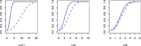
Figure 1: Optimal asymptotic power (26) (in full line) and local asymptotic power of the asymmetry test (17) (in dotted line) when $\eta_{t}$ follows a standardized Student distribution with $\nu$ degrees of freedom. The horizontal axis correspond to the local parameter $\mathbf{e}^{\prime}\bolds{\tau}$.

This point is illustrated by Figure 1, in which the local asymptotic power of the asymmetry test (in dotted lines) is compared to the optimal asymptotic power given by (26). In this figure, the noise $\eta_{t}$ is assumed to satisfy a Student distribution with $\nu>2$ degrees of freedom, standardized in such a way that $E\eta_{t}^{2}=1$. The parameters of the model under the null are $\alpha_{0+}=\alpha_{0-}=0.2$, $\beta_{0}=0.9$ and $\delta=1$, which corresponds to a nonstationary model with $\gamma_{0}=0.045$. In the figure, it can be seen that the local asymptotic power is far from the optimal power when $\nu$ is small, but, as expected, the discrepancy decreases as $\nu$ increases.

6 Estimation when the power $\delta$ is unknown

In this section, we consider the case where the power $\delta$, now denoted $\delta_{0}$, is unknown and is jointly estimated with $\theta_{0}$. We rewrite the vector of parameters as $\zeta:=(\delta,\theta^{\prime})^{\prime}$, which is assumed to belong to a compact parameter space $\Upsilon\subset(0,\infty)^{2}\times[0,\infty)^{3}$. The true parameters value is denoted by $\zeta_{0}:=(\delta_{0},\theta_{0}^{\prime})^{\prime}$. A QMLE of $\zeta$ is defined as any measurable solution $\hat{\zeta}_{n}$ of

$$\quad\hat{\zeta}_{n}=\bigl{(}\hat{\delta}_{n},\hat{\theta}_{n}^{\prime}\bigr{)}^{\prime}=\mathop{\arg\min}_{\zeta\in\Upsilon}\frac{1}{n}\sum_{t=1}^{n}\ell_{t}(\zeta),\qquad\ell_{t}(\zeta)=\frac{\epsilon_{t}^{2}}{\sigma_{t}^{2}(\zeta)}+\log\sigma_{t}^{2}(\zeta),$$ (28)

where

$$\sigma_{t}={\sigma}_{t}(\zeta)=\bigl{(}\omega+\alpha_{+}\bigl{(}\epsilon_{t-1}^{+}\bigr{)}^{\delta}+\alpha_{-}\bigl{(}-\epsilon_{t-1}^{-}\bigr{)}^{\delta}+\beta{\sigma}_{t-1}^{\delta}(\zeta)\bigr{)}^{1/\delta}$$ (29)

for $t=1,\ldots,n$ [with initial values for $\epsilon_{0}$ and $\sigma_{0}(\zeta)$]. The rescaled residuals are defined by $\hat{\eta}_{t}=\eta_{t}(\hat{\zeta}_{n})$ where $\eta_{t}(\zeta)=\epsilon_{t}/\sigma_{t}(\zeta)$ for $t=1,\ldots,n$. For identifiability reasons, we need to slightly reinforce assumption A1 as follows.

A3: The support of $\eta_{t}$ contains at least three points of the same sign, and at least two points of opposite signs.

We also introduce the following technical assumption to handle the derivatives of $\ell_{t}$ with respect to the exponent $\delta$.

A4: $\forall\zeta\in\Upsilon$, $\beta<\|1/a_{0}^{2}(\eta_{1})\|_{p}^{-1}$ and $\||\eta_{1}|^{\delta}\log|\eta_{1}|\|_{p}<\infty$ for some $p>1$.

For brevity, we only present results for the nonstationary cases.

Theorem 6.1

Let (1)–(2) and A3 hold. Then the QMLE defined in (28) satisfies the following properties:

1. [(ii)]

2. Explosive case. When $\gamma_{0}>0$, if $P(\eta_{1}=0)=0$

   $$\bigl{(}\delta_{n},\hat{\vartheta}_{n}^{\prime}\bigr{)}\to\bigl{(}\delta_{0},\vartheta_{0}^{\prime}\bigr{)}\qquad\mbox{a.s. as }n\to\infty.$$

   If, in addition, $\kappa_{\eta}\in(1,\infty)$, $E|\log\eta_{1}^{2}|<\infty$, $\zeta_{0}\in\accentset{\circ}{\Upsilon}$, and A4 holds, then

   $$\sqrt{n}\bigl{(}\bigl{(}\hat{\delta}_{n},\hat{\vartheta}_{n}^{\prime}\bigr{)}-\bigl{(}\delta_{0},\vartheta_{0}^{\prime}\bigr{)}\bigr{)}^{\prime}\stackrel{{\scriptstyle d}}{{\to}}{\cal N}\bigl{\{}0,(\kappa_{\eta}-1){\cal I}_{\delta}^{-1}\bigr{\}}$$ (30)

   as $n\to\infty$, where ${\cal I}_{\delta}$ is a positive definite matrix (see Lemma 3.1).

3. At the boundary of the stationarity region. When $\gamma_{0}=0$, if $P(\eta_{1}=0)=0$, and $\forall\zeta\in\Upsilon$, $\beta<\|1/a_{0}(\eta_{1})\|_{p}^{-1}$ for some $p>1$,

   $$\bigl{(}\delta_{n},\hat{\vartheta}_{n}^{\prime}\bigr{)}\to\bigl{(}\delta_{0},\vartheta_{0}^{\prime}\bigr{)}\qquad\mbox{in probability as }n\to\infty.$$

   If, in addition, $\zeta_{0}\in\accentset{\circ}{\Upsilon}$, $\kappa_{\eta}\in(1,\infty)$, $E|\log\eta_{1}^{2}|<\infty$ and A2 and A4 are satisfied, then (30) holds.

The presence of parameter $\delta$ induces specific difficulties. It turns out that the derivative of the criterion with respect to $\delta$ involves the process $({\partial\sigma_{t}^{\delta}}/{\partial\delta}-\log\sigma_{t})$. A strictly stationary approximation to this process can then be obtained, but in a more complicated way than for the other parameters. To save space, the proofs of this section are given in the supplementary file [Francq and Zakoïan (2013)].

Obviously, stationarity and symmetry tests could be derived as in Sections 4 and 5. Other tests concerning the exponent $\delta$ [e.g., testing the TARCH model ($\delta=1$) against the GJR model ($\delta=2$)] could be considered as well, but we leave this for further investigation.

7 Proofs and complementary results

Proof of Proposition 2.1 Writing $\omega_{t}=\omega(\xi_{t})$ and $a_{t}=a(\xi_{t})$, we have, for all $t>1$ and $1\leq k<t$,

$$h_{t}=\omega_{t-1}+\sum_{j=1}^{k}\omega_{t-j-1}\prod_{i=1}^{j}a_{t-i}+h_{t-k-1}\prod_{i=1}^{k+1}a_{t-i}.$$ (31)

We begin by showing (i). Since all the random variables involved in (31) are positive, $h_{t}\geq\underline{\omega}\prod_{i=1}^{t-1}a_{t-i}$. For any constant $\rho>e^{-\gamma}$, we thus have, a.s.

$$\liminf_{t\to\infty}\frac{1}{t}\log\rho^{t}h_{t}\geq\log\rho+\lim_{t\to\infty}\frac{1}{t}\Biggl{\{}\log\underline{\omega}+\sum_{i=1}^{t-1}\log a_{i}\Biggr{\}}=\log\rho+\gamma>0$$

by the ergodic theorem. It follows that $\log\rho^{t}h_{t}$, and hence $\rho^{t}h_{t}$, tend to $+\infty$ a.s. as $n\to\infty$. The second convergence is shown in just the same way, arguing that $E|\log\xi_{1}^{2}|<\infty$ entails $\log\xi_{t}^{2}/t\to 0$ a.s. as $t\to\infty$.

To show (ii), first consider the case where $h_{0}=0$. Note that, for all $t$, the distribution of $h_{t}=h_{t}(\xi_{0},\ldots,\xi_{t-1})$ is equal to that of

$$h^{*}_{t}:=h_{t}(\xi_{t},\ldots,\xi_{1})=\omega_{1}+\sum_{j=1}^{t-1}\omega_{j+1}\prod_{i=1}^{j}a_{i}.$$ (32)

Note that, contrary to $(h_{t})$, the sequence $(h^{*}_{t})$ increases with $t$. The Chung–Fuchs theorem applied to the random walk $\sum_{i=1}^{t}\log a_{i}$ entails that$\limsup_{t\to\infty}\prod_{i=1}^{t}a_{i}=+\infty$ a.s. It follows that $h^{*}_{t}\to+\infty$ as $t\to\infty$. We thus have $P(h_{t}\geq A)=P(h_{t}^{*}\geq A)\to 1$ for all $A>0$, from which the first part of (ii) easily follows. To prove the first convergence of (4), note that the dominated convergence theorem entails

$$E\psi(h_{t})=\int_{0}^{\infty}P\bigl{\{}h_{t}^{*}<\psi^{-1}(u)\bigr{\}}\,du\to\int_{0}^{\infty}\lim_{t\to\infty}P\bigl{\{}h_{t}^{*}<\psi^{-1}(u)\bigr{\}}\,du=0.$$

The second convergence is shown similarly. Now consider the case where the initial value is not equal to zero. It is clear from (31), with $k=t-1$, that $h_{t}$ is an increasing function of $h_{0}$. So the convergences to infinity obtained when $h_{0}=0$, and the convergences in (4), hold a fortiori when $h_{0}>0$.

7.1 Asymptotic behavior of the QMLE of $\vartheta_{0}$

Define the $[0,\infty]$-valued process

$$v_{t}(\vartheta)=\sum_{j=1}^{\infty}\frac{\{\alpha_{+}(\eta_{t-j}^{+})^{\delta}+\alpha_{-}(-\eta_{t-j}^{-})^{\delta}\}}{a_{0}(\eta_{t-j})}\prod_{k=1}^{j-1}\frac{\beta}{a_{0}(\eta_{t-k})}$$

with the convention $\prod_{k=1}^{j-1}=1$ when $j\leq 1$. Let $\Theta_{0}=\{\theta\in\Theta\dvtx\beta<e^{\gamma_{0}}\}$ and $\Theta_{p}=\{\theta\in[0,\infty)^{4}\dvtx\beta<\|1/a_{0}(\eta_{1})\|_{p}^{-1}\}$.

Lemma 7.1

(i) When $\gamma_{0}>0$, for any $\theta\in\Theta_{0}$ the process $v_{t}(\vartheta)$ is stationary and ergodic. Moreover, for any compact $\Theta_{0}^{*}\subset\Theta_{0}$,

$$\sup_{\theta\in\Theta_{0}^{*}}\biggl{|}\frac{\sigma_{t}^{\delta}(\theta)}{h_{t}}-v_{t}(\vartheta)\biggr{|}\to 0\qquad\mbox{a.s. as $t\to\infty$}.$$

Finally, for any $\theta\notin\Theta_{0}$ it holds that ${\sigma_{t}^{\delta}(\theta)}/{h_{t}}\to\infty$ a.s.

(ii) When $\gamma_{0}=0$, for any $\theta\in\Theta_{p}$ with $p\geq 1$, the process $v_{t}(\vartheta)$ is stationary and ergodic. Moreover, for any compact $\Theta_{p}^{*}\subset\Theta_{p}$,

$$\sup_{\theta\in\Theta_{p}^{*}}\biggl{|}\frac{\sigma_{t}^{\delta}(\theta)}{h_{t}}-v_{t}(\vartheta)\biggr{|}\to 0\qquad\mbox{in $L^{p}$}.$$

Assuming, with no generality loss, that $\sigma_{0}(\theta)=0$, we have $\sigma_{t}^{\delta}(\theta)=\sum_{j=1}^{t}\beta^{j-1}z_{t-j}$ where $z_{t}=\omega+\alpha_{+}(\epsilon_{t}^{+})^{\delta}+\alpha_{-}(-\epsilon_{t}^{-})^{\delta}$ and

$$\frac{\sigma_{t}^{\delta}(\theta)}{h_{t}}=\sum_{j=1}^{t}\beta^{j-1}\Biggl{\{}\prod_{k=1}^{j}\frac{h_{t-k}}{h_{t-k+1}}\Biggr{\}}\frac{z_{t-j}}{h_{t-j}}.$$ (33)

Noting that

$$\frac{h_{t-k}}{h_{t-k+1}}=\frac{h_{t-k}}{\omega_{0}+a_{0}(\eta_{t-k})h_{t-k}}\leq\frac{1}{a_{0}(\eta_{t-k})},$$ (34)

the rest of the proof follows from arguments similar to those used in the proof of Lemma A.1 in FZ. Therefore is it omitted.

Lemma 7.2

If $\theta\in\Theta_{0}$, we have $v_{t}(\vartheta)=1$, a.s. if and only if $\vartheta=\vartheta_{0}$.

Straightforward algebra shows that

$$v_{t}(\vartheta)a_{0}(\eta_{t-1})=\beta v_{t-1}(\vartheta)+\alpha_{+}\bigl{(}\eta_{t-1}^{+}\bigr{)}^{\delta}+\alpha_{-}\bigl{(}-\eta_{t-1}^{-}\bigr{)}^{\delta}.$$ (35)

Hence

$$\bigl{\{}v_{t}(\vartheta)-1\bigr{\}}a_{0}(\eta_{t-1}) = \beta v_{t-1}(\vartheta)-\beta_{0}+(\alpha_{+}-\alpha_{0+})\bigl{(}\eta_{t-1}^{+}\bigr{)}^{\delta}$$

$${}+(\alpha_{-}-\alpha_{0-})\bigl{(}-\eta_{t-1}^{-}\bigr{)}^{\delta}.$$

It follows that $v_{t}(\vartheta)=1$ a.s. if and only if

$$\beta-\beta_{0}+(\alpha_{+}-\alpha_{0+})\bigl{(}\eta_{t-1}^{+}\bigr{)}^{\delta}+(\alpha_{-}-\alpha_{0-})\bigl{(}-\eta_{t-1}^{-}\bigr{)}^{\delta}=0.$$

Thus if $\vartheta\neq\vartheta_{0}$, $\eta_{t}$ takes at most two values of different signs, in contradiction with assumption A1. The conclusion follows.

Let $\underline{\omega}=\inf\{\omega\mid\theta\in\Theta\}$, $\underline{\alpha}=\inf\{\alpha_{+},\alpha_{-}\mid\theta\in\Theta\}$, $\underline{\beta}=\inf\{\beta\mid\theta\in\Theta\}$, $\overline{\omega}=\sup\{\omega\mid\theta\in\Theta\}$, $\overline{\alpha}=\sup\{\alpha_{+},\alpha_{-}\mid\theta\in\Theta\}$, $\overline{\beta}=\sup\{\beta\mid\theta\in\Theta\}$. Denote by $K$ any constant whose value is unimportant and can change throughout the proofs. Let $\check{\Theta}$ be the compact set of the $\vartheta$’s such that $(\omega,\vartheta^{\prime})^{\prime}\in\Theta$.

Lemma 7.3

Suppose that $P(\eta_{t}=0)=0$. Then, for any $k>0$,

$$E\sup_{\vartheta\in\check{\Theta}}\biggl{(}\frac{1}{v_{t}(\vartheta)}\biggr{)}^{k}<\infty\quad\mbox{and}\quad E\sup_{\theta\in\Theta}\biggl{(}\frac{h_{t}}{\sigma_{t}^{\delta}(\theta)}\biggr{)}^{k}<\infty.$$

Let $\varepsilon>0$ such that $p(\varepsilon):=P(|\eta_{t}|\leq\varepsilon)\in[0,1)$. If $|\eta_{t-1}|>\varepsilon$, since the sum $v_{t}(\vartheta)$ is greater than its first term, we have

$$\frac{1}{v_{t}(\vartheta)}\leq\frac{a_{0}(\eta_{t-1})}{\alpha_{+}(\eta_{t-1}^{+})^{\delta}+\alpha_{-}(-\eta_{t-1}^{-})^{\delta}}\leq\frac{\max(\alpha_{0+},\alpha_{0-})}{\underline{\alpha}}+\frac{\beta_{0}}{\underline{\alpha}\varepsilon^{\delta}}:=K(\varepsilon).$$

Iterating this method, we can write

$$\sup_{\vartheta\in\check{\Theta}}\frac{1}{v_{t}(\vartheta)}\leq K(\varepsilon)\sum_{i=1}^{\infty}\mathbh 1_{|\eta_{t-1}|\leq\varepsilon}\cdots\mathbh 1_{|\eta_{t-i+1}|\leq\varepsilon}\mathbh 1_{|\eta_{t-i}|>\varepsilon}\biggl{(}\frac{\overline{a}_{0}(\varepsilon)}{\underline{\beta}}\biggr{)}^{i-1},$$

where $\overline{a}_{0}(\varepsilon)=\max(\alpha_{0+},\alpha_{0-})\epsilon^{\delta}+\beta_{0}$. It follows that, for any integer $k$,

$$E\sup_{\vartheta\in\check{\Theta}}\biggl{(}\frac{1}{v_{t}(\vartheta)}\biggr{)}^{k}\leq\bigl{\{}K(\varepsilon)\bigr{\}}^{k}\bigl{\{}1-p(\varepsilon)\bigr{\}}\sum_{i=1}^{\infty}p(\varepsilon)^{i-1}\biggl{(}\frac{\overline{a}_{0}(\varepsilon)}{\underline{\beta}}\biggr{)}^{k(i-1)}.$$

Noting that $\lim_{\varepsilon\to 0}p(\varepsilon)=0$ and $\lim_{\varepsilon\to 0}\overline{a}_{0}(\varepsilon)=\beta_{0}$, we have $p(\varepsilon)(\frac{\overline{a}_{0}(\varepsilon)}{\underline{\beta}})^{k}<1$ for $\varepsilon$ sufficiently small. The first result of the lemma is thus proven.

Similarly, we have for $|\eta_{t-1}|>\varepsilon$,

$$\frac{h_{t}}{\sigma_{t}^{\delta}(\theta)}\leq\frac{\omega_{0}}{\underline{\omega}}+\frac{\overline{\alpha}}{\underline{\alpha}}+\frac{\beta_{0}}{\underline{\alpha}\varepsilon^{\delta}}:=H(\varepsilon)$$

and for $|\eta_{t-1}|\leq\varepsilon$ and $|\eta_{t-2}|>\varepsilon$,

$$\frac{h_{t}}{\sigma_{t}^{\delta}(\theta)}\leq\frac{\omega_{0}}{\underline{\omega}}+\frac{\overline{a}_{0}(\varepsilon)}{\underline{\beta}}H(\varepsilon).$$

More generally,

$$\sup_{\theta\in\Theta}\frac{h_{t}}{\sigma_{t}^{\delta}(\theta)} \leq \sum_{i=1}^{\infty}\mathbh 1_{|\eta_{t-1}|\leq\varepsilon}\cdots\mathbh 1_{|\eta_{t-i+1}|\leq\varepsilon}\mathbh 1_{|\eta_{t-i}|>\varepsilon}$$

$$\hskip 12.9pt{}\times\Biggl{(}\frac{\omega_{0}}{\underline{\omega}}\sum_{j=0}^{i-2}\biggl{(}\frac{\overline{a}_{0}(\varepsilon)}{\underline{\beta}}\biggr{)}^{j}+\biggl{(}\frac{\overline{a}_{0}(\varepsilon)}{\underline{\beta}}\biggr{)}^{i-1}H(\varepsilon)\Biggr{)}.$$

The conclusion follows by the same arguments as before.

Proof of the consistency results in cases (ii) and (iii) of Theorem 3.1 Note that $(\hat{\omega}_{n},\hat{\vartheta}_{n}^{\prime})=\mathop{\arg\min}_{\theta\in\Theta}Q_{n}(\theta)$, where $Q_{n}(\theta)=n^{-1}\*\sum_{t=1}^{n}\{\ell_{t}(\theta)-\ell_{t}(\theta_{0})\}$. We have

$$Q_{n}(\theta)=\frac{1}{n}\sum_{t=1}^{n}\eta_{t}^{2}\biggl{\{}\biggl{(}\frac{h_{t}}{\sigma_{t}^{\delta}(\theta)}\biggr{)}^{2/{\delta}}-1\biggr{\}}+\log\biggl{(}\frac{\sigma_{t}^{\delta}(\theta)}{h_{t}}\biggr{)}^{2/{\delta}}=O_{n}(\vartheta)+R_{n}(\theta),$$

where

$$O_{n}(\vartheta)=\frac{1}{n}\sum_{t=1}^{n}\eta_{t}^{2}\biggl{\{}\frac{1}{v_{t}^{2/{\delta}}(\vartheta)}-1\biggr{\}}+\log v_{t}^{2/{\delta}}(\vartheta)$$

and

$$R_{n}(\theta)=\frac{1}{n}\sum_{t=1}^{n}\eta_{t}^{2}\biggl{\{}\biggl{(}\frac{h_{t}}{\sigma_{t}^{\delta}(\theta)}\biggr{)}^{2/{\delta}}-\frac{1}{v_{t}^{2/{\delta}}(\vartheta)}\biggr{\}}+\log\biggl{(}\frac{\sigma_{t}^{\delta}(\theta)}{h_{t}v_{t}(\vartheta)}\biggr{)}^{2/{\delta}}.$$

It suffices to consider the case $\theta\in\Theta^{*}_{0}$ where $\Theta^{*}_{0}$ is an arbitrary compact subset of $\Theta_{0}$, because by Lemma 7.1(i) $Q_{n}(\theta)\to\infty$ a.s. if $\theta\notin\Theta_{0}$. We have by stationarity and ergodicity of $v_{t}(\vartheta)$, a.s.

$$\lim_{n\to\infty}O_{n}(\vartheta)=E\biggl{\{}\frac{1}{v_{1}^{2/{\delta}}(\vartheta)}-1+\log v_{1}^{2/{\delta}}(\vartheta)\biggr{\}}\geq 0,$$

because $\log x\leq x-1$ for $x>0$. The inequality is strict except when $v_{1}(\vartheta)=1$ a.s. By Lemma 7.2 we thus have $E\{O_{n}(\vartheta)\}\geq 0$, with equality only if $\vartheta=\vartheta_{0}$.

By Lemma 7.3 we prove, as in FZ, that

$$\qquad\lim_{n\to\infty}\sup_{\theta\in\Theta_{0}^{*}}\bigl{|}R_{n}(\theta)\bigr{|}=0\qquad\mbox{a.s. }\Bigl{[}\mbox{resp., }\lim_{n\to\infty}\sup_{\theta\in\Theta_{p}^{*}}\bigl{|}R_{n}(\theta)\bigr{|}=0\mbox{ in }L^{1}\Bigr{]},$$ (36)

when $\gamma_{0}>0$ (resp., $\gamma_{0}=0$) and $\Theta_{0}^{*},\Theta_{p}^{*}$ are defined in Lemma 7.1, which completes the proof.

We now need to introduce new $[0,\infty]$-valued processes. Let $a(\eta_{t})=\break\alpha_{+}(\eta_{t}^{+})^{\delta}+\alpha_{-}(-\eta_{t}^{-})^{\delta}+\beta$ and

$$d_{t}^{\alpha_{+}} = \sum_{j=1}^{\infty}\frac{(\eta_{t-j}^{+})^{\delta}}{a_{0}(\eta_{t-j})}\prod_{k=1}^{j-1}\frac{\beta_{0}}{a_{0}(\eta_{t-k})},\qquad d_{t}^{\alpha_{-}}=\sum_{j=1}^{\infty}\frac{(-\eta_{t-j}^{-})^{\delta}}{a_{0}(\eta_{t-j})}\prod_{k=1}^{j-1}\frac{\beta_{0}}{a_{0}(\eta_{t-k})},$$

$$d_{t}^{\beta} = \sum_{j=2}^{\infty}\frac{(j-1)\{\alpha_{0+}(\eta_{t-j}^{+})^{\delta}+\alpha_{0-}(-\eta_{t-j}^{-})^{\delta}\}}{\beta_{0}a_{0}(\eta_{t-j})}\prod_{k=1}^{j-1}\frac{\beta_{0}}{a_{0}(\eta_{t-k})}.$$

Lemma 7.4

Assume $\gamma_{0}\geq 0$ and $E\eta_{t}^{4}<\infty$. We have

$$\frac{1}{\sqrt{n}}\sum_{t=1}^{n}\frac{\partial\ell_{t}}{\partial\vartheta}(\theta_{0})\stackrel{{\scriptstyle d}}{{\to}}{\cal N}\bigl{\{}0,(\kappa_{\eta}-1){\cal I}\bigr{\}}\qquad\mbox{as $n\to\infty$},$$

where ${\cal I}=\frac{4}{\delta^{2}}Ed_{1}d_{1}^{\prime}$ and $d_{t}^{\prime}=(d_{t}^{\alpha_{+}},d_{t}^{\alpha_{-}},d_{t}^{\beta})$. Moreover, ${\cal I}$ is nonsingular.

Since $E\log\beta_{0}/a_{0}(\eta_{1})<0$, by the Cauchy root test, the processes $d_{t}^{\alpha_{+}},d_{t}^{\alpha_{-}}$ and $d_{t}^{\beta}$ are stationary and ergodic. Still assuming $\sigma_{0}^{2}=0$, we have

$$\frac{\partial\sigma_{t}^{\delta}}{\partial(\alpha_{+},\alpha_{-})}(\theta) = \sum_{j=1}^{t}\beta^{j-1}\bigl{(}\bigl{\{}\epsilon_{t-j}^{+}\bigr{\}}^{\delta},\bigl{\{}-\epsilon_{t-j}^{-}\bigr{\}}^{\delta}\bigr{)},$$

$$\frac{\partial\sigma_{t}^{2}}{\partial\beta}(\theta) = \sum_{j=2}^{t}(j-1)\beta^{j-2}z_{t-j}.$$

Thus, using a direct extension of (34),

$$\frac{1}{\sigma^{\delta}_{t}(\theta_{0})}\,\frac{\partial\sigma_{t}^{\delta}}{\partial(\alpha_{+},\alpha_{-})}(\theta_{0}) = \sum_{j=1}^{t}\beta^{j-1}\Biggl{\{}\prod_{k=1}^{j}\frac{\sigma^{\delta}_{t-k}(\theta_{0})}{\sigma^{\delta}_{t-k+1}(\theta_{0})}\Biggr{\}}\frac{\{(\epsilon_{t-j}^{+})^{\delta},(-\epsilon_{t-j}^{-})^{\delta}\}}{\sigma^{\delta}_{t-j}(\theta_{0})}$$

$$\leq \bigl{(}d_{t}^{\alpha_{+}}(\vartheta_{0}),d_{t}^{\alpha_{-}}(\vartheta_{0})\bigr{)},$$

$$\frac{1}{\sigma^{\delta}_{t}(\theta_{0})}\,\frac{\partial\sigma_{t}^{\delta}}{\partial\beta}(\theta_{0}) = \sum_{j=2}^{t}(j-1)\beta_{0}^{j-2}\Biggl{\{}\prod_{k=1}^{j}\frac{\sigma^{\delta}_{t-k}(\theta_{0})}{\sigma^{\delta}_{t-k+1}(\theta_{0})}\Biggr{\}}\frac{z_{t-j}}{\sigma^{\delta}_{t-j}(\theta_{0})}$$

$$\leq d_{t}^{\beta}(\vartheta_{0}),$$

where the first inequality stands componentwise. Moreover, we have

$$0\leq d_{t}^{\alpha_{+}}(\vartheta_{0})-\frac{1}{\sigma^{\delta}_{t}}\frac{\partial\sigma_{t}^{\delta}}{\partial\alpha^{+}}(\theta_{0})\leq s_{t_{0}}+r_{t_{0}},$$

where

$$s_{t_{0}} = \sum_{j=1}^{t_{0}}\frac{(\eta_{t-j}^{+})^{\delta}}{a_{0}(\eta_{t-j})}\prod_{k=1}^{j-1}\frac{\beta_{0}}{a_{0}(\eta_{t-k})}-\frac{(\epsilon_{t-j}^{+})^{\delta}}{\beta_{0}\sigma^{\delta}_{t-j}(\theta_{0})}\prod_{k=1}^{j}\frac{\beta_{0}\sigma^{\delta}_{t-k}(\theta_{0})}{\sigma^{\delta}_{t-k+1}(\theta_{0})},$$

$$r_{t_{0}} = \sum_{j=t_{0}+1}^{\infty}\frac{(\eta_{t-j}^{+})^{\delta}}{a_{0}(\eta_{t-j})}\prod_{k=1}^{j-1}\frac{\beta_{0}}{a_{0}(\eta_{t-k})}.$$

For all $p\geq 1$, $\|r_{t_{0}}\|_{p}\to 0$ as $t_{0}\to\infty$ because $\|\beta_{0}/a_{0}(\eta_{1})\|_{p}<1$ and $\|(\eta_{1}^{+})^{\delta}/\break a_{0}(\eta_{1})\|_{p}<1/\alpha_{0+}$. Since, in addition, $\|\beta_{0}\sigma_{t-1}^{\delta}(\theta_{0})/\sigma^{\delta}_{t}(\theta_{0})\|_{p}<1$, and

$$\biggl{\|}\frac{\beta_{0}}{a_{0}(\eta_{t-1})}-\frac{\beta_{0}\sigma_{t-1}^{\delta}(\theta_{0})}{\sigma^{\delta}_{t}(\theta_{0})}\biggr{\|}_{p}=\biggl{\|}\frac{\beta_{0}\omega_{0}}{a_{0}(\eta_{t-1})\sigma^{\delta}_{t}(\theta_{0})}\biggr{\|}_{p}\to 0$$

as $t\to\infty$ by the dominated convergence theorem, $s_{t_{0}}=s_{t_{0}}(t)$ converges to 0 in $L^{p}$ as $t\to\infty$. The same derivations hold true when $d_{t}^{\alpha_{+}}$ is replaced by $d_{t}^{\alpha_{-}}$ and $d_{t}^{\beta}$. Therefore, $d_{t}^{\alpha_{+}},d_{t}^{\alpha_{-}}$ and $d_{t}^{\beta}$ have moments of any order, and

$$\biggl{\|}\frac{1}{\sigma^{\delta}_{t}}\,\frac{\partial\sigma_{t}^{\delta}}{\partial\vartheta}(\theta_{0})-d_{t}\biggr{\|}\to 0$$ (37)

in $L^{p}$ for any $p\geq 1$.

Using (37) and the ergodic theorem, we thus have, as $n\to\infty$,

$$\operatorname{Var}\frac{1}{\sqrt{n}}\sum_{t=1}^{n}\frac{\partial}{\partial\vartheta}\ell_{t}(\theta_{0})=\frac{4}{\delta^{2}}\frac{\kappa_{\eta}-1}{n}\sum_{t=1}^{n}E\bigl{(}d_{t}d_{t}^{\prime}\bigr{)}+o(1)\to(\kappa_{\eta}-1){\cal I}.$$

Moreover, it can be shown as in FZ that the Lindeberg condition is satisfied, allowing us to apply the Lindeberg central limit theorem for martingale differences; see Billingsley (1995), page 476.

Now we show that ${\cal I}$ is nonsingular. Suppose there exists $x=(x_{1},x_{2},x_{3})^{\prime}\in\mathbb{R}^{3}$ such that $x^{\prime}{\cal I}x=0$. Then we get $x^{\prime}d_{t}=0$, that is,

$$\sum_{j=1}^{\infty}\biggl{(}x_{1}\frac{(\eta_{t-j}^{+})^{\delta}}{a(\eta_{t-j})}+x_{2}\frac{(-\eta_{t-j}^{-})^{\delta}}{a(\eta_{t-j})}+x_{3}(j-1)\frac{\alpha_{+}(\eta_{t-j}^{+})^{\delta}+\alpha_{-}(-\eta_{t-j}^{-})^{\delta}}{\beta a(\eta_{t-j})}\biggr{)}$$

$$\qquad{}\times\prod_{k=1}^{j-1}\frac{\beta}{a(\eta_{t-k})}=0\qquad\mbox{a.s.}$$

It follows that $x_{1}(\eta_{t-1}^{+})^{\delta}+x_{2}(-\eta_{t-1}^{-})^{\delta}=z_{t-2}$, a.s. where $z_{t-2}$ is a measurable function of the $\eta_{t-j}$ with $j>1$. Because $\eta_{t-1}$ is independent of $z_{t-2}$, this variable must be a.s. constant. In view of assumption A1, this entails $x_{1}=x_{2}=0$ and then $x_{3}=0$. Therefore, ${\cal I}$ is nonsingular.

Lemma 7.5

Let $\varpi$ be an arbitrary compact subset of $[0,\infty)$. Assume that $E\log\eta_{1}^{2}<\infty$. When $\gamma_{0}>0$ we have, a.s.

$$\sum_{t=1}^{\infty}\sup_{\theta\in\Theta_{0}}\biggl{|}\frac{\partial}{\partial\omega}\ell_{t}(\theta)\biggr{|} < \infty,\qquad\sum_{t=1}^{\infty}\sup_{\theta\in\Theta_{0}}\biggl{\|}\frac{\partial^{2}}{\partial\omega\,\partial\theta}\ell_{t}(\theta)\biggr{\|}<\infty,$$

$$\sup_{\omega\in\varpi}\Biggl{|}\frac{1}{n}\sum_{t=1}^{n}\frac{\partial^{2}\ell_{t}(\omega,\vartheta_{0})}{\partial\theta_{i+1}\,\partial\theta_{j+1}}-{\cal I}_{ij}\Biggr{|} = o(1)\qquad\mbox{for all }i,j\in\{1,2,3\},$$

$$\frac{1}{n}\sum_{t=1}^{n}\sup_{\theta\in\Theta}\biggl{|}\frac{\partial^{3}}{\partial\theta_{i}\,\partial\theta_{j}\,\partial\theta_{k}}\ell_{t}(\theta)\biggr{|} = O(1)\qquad\mbox{for all }i,j,k\in\{2,3,4\}.$$

When $\gamma_{0}=0$ we have, for all $i,j,k\in\{2,3,4\}$,

$$\sup_{\omega\in\varpi}\Biggl{|}\frac{1}{n}\sum_{t=1}^{n}\frac{\partial^{2}\ell_{t}(\omega,\alpha_{0},\beta_{0})}{\partial\theta_{i+1}\,\partial\theta_{j+1}}-{\cal I}_{ij}\Biggr{|} = o_{P}(1),$$ (38)

$$\frac{1}{n}\sum_{t=1}^{n}\sup_{\theta\in\Theta_{4}}\biggl{|}\frac{\partial^{3}}{\partial\theta_{i}\,\partial\theta_{j}\,\partial\theta_{k}}\ell_{t}(\theta)\biggr{|} = O_{P}(1).$$ (39)

This is similar to that of Lemma A.5. in FZ, therefore is it omitted.

Proof of the asymptotic normality in case (ii) of Theorem 3.1 An expansion of the criterion derivative gives

$$\pmatrix{\frac{1}{\sqrt{n}}\sum_{t=1}^{n}\frac{\partial}{\partial\omega}\ell_{t}(\hat{\theta}_{n})\cr 0}=\frac{1}{\sqrt{n}}\sum_{t=1}^{n}\frac{\partial}{\partial\theta}\ell_{t}(\theta_{0})+{\cal J}_{n}\sqrt{n}(\hat{\theta}_{n}-\theta_{0}),$$ (40)

where ${\cal J}_{n}$ is a $4\times 4$ matrix whose elements have the form

$${\cal J}_{n}(i,j)=\frac{1}{n}\sum_{t=1}^{n}\frac{\partial^{2}}{\partial\theta_{i}\,\partial\theta_{j}}\ell_{t}\bigl{(}\theta_{i}^{*}\bigr{)},$$

where $\theta^{*}_{i}=(\omega_{i}^{*},\alpha_{i+}^{*},\alpha_{i-}^{*},\beta_{i}^{*})^{\prime}$ is between $\hat{\theta}_{n}$ and $\theta_{0}$. Moreover, it can be shown that, for $i,j=1,2,3$,

$$\quad{\cal J}_{n}(i+1,1)=o(1/\sqrt{n}),\qquad{\cal J}_{n}(i+1,j+1)\to{\cal I}(i,j)\qquad\mbox{a.s.}$$ (41)

The conclusion follows from the last rows of (40) and Lemma 7.4.

Proof of the asymptotic normality in case (iii) of Theorem 3.1 Note that (40) continues to hold. In view of (38)–(39), we have

$${\cal J}_{n}(i+1,j+1)\to{\cal I}(i,j)\qquad\mbox{in probability as }n\to\infty.$$

To conclude, by the arguments used in case (ii), it suffices to show that

$$\quad\mbox{for $i=2,3,4$}\qquad E\bigl{|}{\cal J}_{n}(i,1)\sqrt{n}(\hat{\omega}_{n}-\omega_{0})\bigr{|}\to 0\qquad\mbox{as }n\to\infty.$$ (42)

Noting that

$$\frac{1}{\sigma_{t}^{\delta}(\theta)}\sum_{j=1}^{t}\beta^{j-1}\bigl{(}\epsilon_{t-j}^{+}\bigr{)}^{\delta}\leq\frac{1}{\alpha_{+}},$$ (43)

and $\beta_{2}^{*}<1$ for $n$ large enough, and using the compactness of $\Theta$, we obtain

$$\bigl{|}{\cal J}_{n}(2,1)\sqrt{n}(\hat{\omega}_{n}-\omega_{0})\bigr{|}$$

$$\qquad\leq\frac{K}{\sqrt{n}}\sum_{t=1}^{n}\biggl{(}\frac{2h_{t}^{2/\delta}\eta_{t}^{2}}{\sigma_{t}^{2}(\theta^{*}_{2})}+1\biggr{)}\frac{\{\sum_{j=1}^{t}(\beta_{2}^{*})^{j-1}(\epsilon_{t-j}^{+})^{\delta}\}\{\sum_{j=1}^{t}(\beta_{2}^{*})^{j-1}\}}{\sigma_{t}^{2\delta}(\theta^{*}_{2})}$$

$$\qquad\leq\frac{K}{\sqrt{n}}\sum_{t=1}^{n}\biggl{(}\frac{2h_{t}^{2/\delta}\eta_{t}^{2}}{\sigma_{t}^{2}(\theta^{*}_{2})}+1\biggr{)}\frac{h_{t}}{\sigma_{t}^{\delta}(\theta^{*}_{2})}\frac{1}{h_{t}}.$$

Hence, by Lemma 7.3 and Hölder’s inequality

$$E\bigl{|}{\cal J}_{n}(2,1)\sqrt{n}(\hat{\omega}_{n}-\omega_{0})\bigr{|}\leq\frac{K}{\sqrt{n}}\sum_{t=1}^{n}E\frac{1}{h_{t}^{1+\tau}}$$

for any $\tau>0$. The same bound is obtained when ${\cal J}_{n}(2,1)$ is replaced by ${\cal J}_{n}(3,1)$ and ${\cal J}_{n}(4,1)$. Moreover,

$$h_{t}=\omega_{0}(1+Z_{t-1}+Z_{t-1}Z_{t-2}+\cdots+Z_{t-1}\cdots Z_{1})+Z_{t-1}\cdots Z_{0}\sigma_{0}^{2}.$$

Hence

$$\frac{1}{h_{t}^{1+\tau}}\leq\frac{1}{\omega_{0}^{1+\tau}(1+Z_{t-1}+Z_{t-1}Z_{t-2}+\cdots+Z_{t-1}\cdots Z_{1})}.$$

By assumption A2, the conclusion follows.

Proof of Theorem 3.2 To save space, this is displayed in the supplementary file [Francq and Zakoïan (2013)].

7.2 Stationarity test

Proof of Theorem 4.1 In the stationary case $\gamma_{0}<0$, standard arguments show that

$$\hat{\gamma}_{n}={\gamma}_{n}(\theta_{0})+\frac{\partial{\gamma}_{n}(\theta_{0})}{\partial\theta^{\prime}}(\hat{\theta}_{n}-\theta_{0})+o_{P}\bigl{(}n^{-1/2}\bigr{)}$$ (44)

with

$$\quad\frac{\partial{\gamma}_{n}(\theta_{0})}{\partial\theta} = \frac{-1}{n}\sum_{t=1}^{n}\frac{1}{a_{0}(\eta_{t})}\left[\bigl{\{}a_{0}(\eta_{t})-\beta_{0}\bigr{\}}\frac{1}{h_{t}}\frac{\partial\sigma^{\delta}_{t}(\theta_{0})}{\partial\theta}-\pmatrix{0\cr\bigl{(}\eta^{+}_{t}\bigr{)}^{\delta}\cr\bigl{(}-\eta^{-}_{t}\bigr{)}^{\delta}\cr 1}\right]$$

$$= -\Psi+o_{P}(1),$$

where $\Psi=(1-\nu_{1})\Omega-a$ and $\Omega=E_{\infty}\frac{1}{h_{t}}\,\frac{\partial\sigma_{t}^{\delta}(\theta_{0})}{\partial\theta}$. Moreover the QMLE satisfies

$$\sqrt{n}(\hat{\theta}_{n}-\theta_{0})=-{\cal J}^{-1}\frac{1}{\sqrt{n}}\sum_{t=1}^{n}\bigl{(}1-\eta_{t}^{2}\bigr{)}\frac{2}{\delta h_{t}}\,\frac{\partial\sigma_{t}^{\delta}(\theta_{0})}{\partial\theta}+o_{P}(1).$$ (46)

In view of (44), (7.2) and (46), we have

$$\sqrt{n}(\hat{\gamma}_{n}-\gamma_{0})=\frac{1}{\sqrt{n}}\sum_{t=1}^{n}u_{t}+\Psi^{\prime}{\cal J}^{-1}\frac{1}{\sqrt{n}}\sum_{t=1}^{n}\bigl{(}1-\eta_{t}^{2}\bigr{)}\frac{2}{\delta h_{t}}\,\frac{\partial\sigma_{t}^{\delta}(\theta_{0})}{\partial\theta}+o_{P}(1).$$

Note that

$$\operatorname{Cov}\Biggl{(}\frac{1}{\sqrt{n}}\sum_{t=1}^{n}u_{t},\Psi^{\prime}{\cal J}^{-1}\frac{1}{\sqrt{n}}\sum_{t=1}^{n}\bigl{(}1-\eta_{t}^{2}\bigr{)}\frac{2}{\delta h_{t}}\,\frac{\partial\sigma_{t}^{\delta}(\theta_{0})}{\partial\theta}\Biggr{)}=\frac{2c}{\delta}\Omega^{\prime}{\cal J}^{-1}\Psi,$$

where $c=\operatorname{Cov}(u_{t},1-\eta_{t}^{2})$. The Slutsky lemma and the central limit theorem for martingale differences thus entail

$$\sqrt{n}(\hat{\gamma}_{n}-\gamma_{0})\stackrel{{\scriptstyle d}}{{\to}}{\cal N}\biggl{(}0,\sigma^{2}_{u}+4\frac{c}{\delta}\Omega^{\prime}{\cal J}^{-1}\Psi+(\kappa_{\eta}-1)\Psi^{\prime}{\cal J}^{-1}\Psi\biggr{)}.$$

Now let $\overline{\theta}_{0}=(\omega_{0},\alpha_{0+},\alpha_{0-},0)^{\prime}$. Noting that $\overline{\theta}_{0}^{\prime}\,\partial\sigma_{t}^{\delta}(\theta_{0})/\partial\theta=h_{t}$ almost surely, we have

$$E\biggl{\{}\frac{1}{h_{t}}\,\frac{\partial\sigma_{t}^{\delta}(\theta_{0})}{\partial\theta}\biggl{(}1-\frac{1}{h_{t}}\frac{\partial\sigma_{t}^{\delta}(\theta_{0})}{\partial\theta^{\prime}}\overline{\theta}_{0}\biggr{)}\biggr{\}}=0,$$

which entails $\frac{\delta^{2}}{4}{\cal J}\overline{\theta}_{0}=\Omega$ and $\Omega^{\prime}{\cal J}^{-1}\Omega=\frac{\delta^{2}}{4}$. It follows that

$$\Omega^{\prime}{\cal J}^{-1}\Psi=(1-\nu_{1})\frac{\delta^{2}}{4}-\frac{\delta^{2}}{4}\overline{\theta}_{0}^{\prime}a=\frac{\delta^{2}}{4}(1-\nu_{1}-\alpha_{0+}\tilde{\nu}_{1+}-\alpha_{0-}\tilde{\nu}_{1-})=0.$$

We also have $\Psi^{\prime}{\cal J}^{-1}\Psi=a^{\prime}{\cal J}^{-1}a-(1-\nu_{1})^{2}$, which completes the proof of the asymptotic distribution (14) in the case $\gamma_{0}<0$.

Now consider the case $\gamma_{0}\geq 0$. Let $\theta_{n}^{*}$ be a sequence such that $\|\theta_{n}^{*}-\theta_{0}\|\leq\|\hat{\theta}_{n}-\theta_{0}\|$. By Proposition 2.1 (using assumption A2 when $\gamma_{0}=0$), we have

$$\frac{1}{\sqrt{n}}\sum_{t=1}^{n}\frac{1}{\sigma_{t}^{\delta}(\theta_{n}^{*})}\frac{\partial\sigma_{t}^{\delta}(\theta_{n}^{*})}{\partial\omega}=o(1)\qquad\mbox{a.s. (resp., in probability) as $n\to\infty$,}$$

when $\gamma_{0}>0$ (resp., when $\gamma_{0}=0$). It can be deduced that, under the same conditions, $\sqrt{n}\,\frac{\partial^{2}\gamma_{n}(\theta_{n}^{*})}{\partial\omega\,\partial\theta}=o(1)$, and $\sqrt{n}(\hat{\theta}-\theta_{0})^{\prime}\,\frac{\partial^{2}\gamma_{n}(\theta_{n}^{*})}{\partial\theta\,\partial\theta^{\prime}}(\hat{\theta}-\theta_{0})=o(1)$, which entails that (44) still holds. The previous arguments show that (7.2) holds with

$$\Omega=E\pmatrix{0\cr d_{t}^{\alpha_{+}}(\theta_{0})\cr d_{t}^{\alpha_{-}}(\theta_{0})\cr d_{t}^{\beta}(\theta_{0})}=\frac{1}{1-\nu_{1}}\pmatrix{0\cr\tilde{\nu}_{1+}\cr\tilde{\nu}_{1-}\cr\nu_{1}/\beta}\quad\mbox{and}\quad\Psi=\pmatrix{0\cr 0\cr 0}.$$

The conclusion follows.

7.3 Asymptotic local powers

Proof of Proposition 5.1 The LAN of GARCH models has already been established in the stationary case; see Drost and Klaassen (1997), Lee and Taniguchi (2005). The nonstationary case will be studied under more general assumptions in the proof of Proposition 5.2.

Proof of Proposition 5.2 Let the functions

$$g_{1}(y)=1+y\frac{f^{\prime}}{f}(y)\quad\mbox{and}\quad g_{2}(y)=1+2y\frac{f^{\prime}}{f}(y)+y^{2}\biggl{(}\frac{f^{\prime}}{f}\biggr{)}^{\prime}(y).$$

Introduce also the notation

$$\Delta_{1,t}(\theta)=\frac{1}{\sigma_{t}(\theta)}\,\frac{\partial^{2}\sigma_{t}(\theta)}{\partial\theta\,\partial\theta^{\prime}},\qquad\Delta_{2,t}(\theta)=\frac{1}{\delta^{2}\sigma_{t}^{2\delta}(\theta)}\,\frac{\partial\sigma_{t}^{\delta}(\theta)}{\partial\theta}\,\frac{\partial\sigma_{t}^{\delta}(\theta)}{\partial\theta^{\prime}}.$$

A Taylor expansion of $\theta_{n}\mapsto\Lambda_{n,f}(\theta_{n},\theta_{0})$ around $\theta_{0}$ yields

$$\Lambda_{n,f}(\theta_{n},\theta_{0})={\bolds{\tau}^{\prime}}S_{n,f}(\theta_{0})-\tfrac{1}{2}\bolds{\tau}^{\prime}\mathfrak{I}_{n}\bigl{(}\theta_{n}^{*}\bigr{)}\bolds{\tau}+{\cal R}_{n},$$ (47)

where $\theta_{n}^{*}$ is between $\theta_{0}$ and $\theta_{n}$,

$$\quad S_{n,f}(\theta_{0}) = \frac{-1}{\sqrt{n}}\sum_{t=1}^{n}g_{1}(\eta_{t})\frac{1}{\delta h_{t}}\,\frac{\partial\sigma_{t}^{\delta}(\theta_{0})}{\partial\theta},$$

$$\mathfrak{I}_{n}(\theta) = \frac{1}{n}\sum_{t=1}^{n}g_{1}\biggl{(}\frac{\epsilon_{t}}{\sigma_{t}(\theta)}\biggr{)}\Delta_{1,t}(\theta)-\frac{1}{n}\sum_{t=1}^{n}g_{2}\biggl{(}\frac{\epsilon_{t}}{\sigma_{t}(\theta)}\biggr{)}\Delta_{2,t}(\theta),$$

and ${\cal R}_{n}$ is a reminder which is displayed below. As in the proof of Lemma 7.4, it can be seen that

$$S_{n,f}(\theta_{0})=\frac{-1}{\delta\sqrt{n}}\sum_{t=1}^{n}g_{1}(\eta_{t})\,d_{t}(\vartheta_{0})+o_{P}(1),\qquad d_{t}(\vartheta)=\pmatrix{0\cr d_{t}^{\alpha_{+}}\cr d_{t}^{\alpha_{-}}\cr d_{t}^{\beta}}.$$

Using (18), it is easy to see that $Eg_{1}(\eta_{1})=0$, and thus $Eg_{1}^{2}(\eta_{1})=\iota_{f}$. The Lindeberg central limit theorem for martingale differences then shows that

$$S_{n,f}(\theta_{0})\stackrel{{\scriptstyle d}}{{\longrightarrow}}{\cal N}(0,\mathfrak{I}_{f}).$$ (49)

Turning to the second term of (47) we first note that, similar to (37),

$$\biggl{|}\frac{1}{h_{t}}\,\frac{\partial\sigma^{\delta}_{t}(\theta_{0})}{\partial\theta}-d_{t}(\vartheta_{0})\biggr{|}\to 0\qquad\mbox{in $L^{2}$ as }t\to\infty.$$

Moreover, integrations by parts show that, under (18), $\int y^{2}f^{\prime\prime}(y)\,dy=\break-2\int y\*f^{\prime}(y)\,dy=2$. It follows that $Eg_{2}(\eta_{1})=-\iota_{f}$. We thus have, using$Eg_{1}(\eta_{1})=0$,

$$\mathfrak{I}_{n}(\theta_{0}) = \frac{1}{n}\sum_{t=1}^{n}\frac{-g_{2}(\eta_{t})}{\delta^{2}}\,d_{t}(\vartheta_{0})\,d_{t}^{\prime}(\vartheta_{0})$$

$${}+o_{P_{\theta_{0}}}(1)\to\mathfrak{I}_{f}\qquad\mbox{in probability as }n\to\infty.$$

Next, it can be shown that, as $n\to\infty$,

$$\bigl{\|}\mathfrak{I}_{n}\bigl{(}\theta_{n}^{*}\bigr{)}-\mathfrak{I}_{n}(\theta_{0})\bigr{\|}\to 0\qquad\mbox{in probability.}$$ (50)

Finally, we show the convergence in probability to zero of

$${\cal R}_{n}=\upsilon_{n}\sum_{t=1}^{n}g_{1}(\eta_{t})\frac{1}{\delta h_{t}}\,\frac{\partial\sigma_{t}^{\delta}(\theta_{0})}{\partial\omega}-\upsilon_{n}\sqrt{n}\bolds{\tau}^{\prime}\mathfrak{I}_{n}\bigl{(}\theta_{n}^{*}\bigr{)}\mathbf{e}_{1}^{\prime}-\frac{1}{2}n\upsilon_{n}^{2}\mathbf{e}_{1}\mathfrak{I}_{n}\bigl{(}\theta_{n}^{*}\bigr{)}\mathbf{e}_{1}^{\prime}.$$

Noting that ${\partial\sigma_{t}^{\delta}(\theta_{0})}/{\partial\omega}$ is constant and that $1/h_{t}$ converges to 0 in $L^{2}$ by Proposition 2.1, the first term in the right-hand side converges to zero in probability. The two other terms can be handled similarly. The conclusion then follows from (47)–(50).

Proof of Proposition 5.3 For simplicity, write $P$ instead of $P_{n,0}$. In the proof of Theorem 4.1 we have seen that

$$T_{n}=\frac{1}{\sqrt{n}}\sum_{t=1}^{n}\frac{u_{t}}{\sigma_{u}}+o_{P}(1).$$

By (22) and (7.3), it follows that under $P$

$$\pmatrix{T_{n}\cr\Lambda_{n,f}(\theta_{0}+\bolds{\tau}/\sqrt{n},\theta_{0})}\stackrel{{\scriptstyle d}}{{\longrightarrow}}{\cal N}\left\{\pmatrix{0\vspace*{2pt}\cr-\dfrac{\iota_{f}}{8}\tilde{\bolds{\tau}}^{\prime}{\cal I}\tilde{\bolds{\tau}}},\pmatrix{1&c\vspace*{2pt}\cr c&\dfrac{\iota_{f}}{4}\tilde{\bolds{\tau}}^{\prime}{\cal I}\tilde{\bolds{\tau}}}\right\},$$

where $\tilde{\bolds{\tau}}^{\prime}=(\tau_{2},\tau_{3},\tau_{4})$, $c=-\frac{\bolds{\tau}^{\prime}Ed_{1}(\vartheta_{0})}{\delta\sigma_{u}}Eu_{1}g_{1}(\eta_{1})=c_{f}(\theta_{0})$. Le Cam’s third lemma [see, e.g., van der Vaart (1998), page 90] shows that

$$T_{n}\stackrel{{\scriptstyle d}}{{\longrightarrow}}{\cal N}\bigl{(}c_{f}(\theta_{0}),1\bigr{)}\qquad\mbox{under }P_{n,\bolds{\tau}}.$$

The conclusion easily follows.

Proof of Proposition 5.4 First consider the case $\gamma_{0}\geq 0$. In the proof of (8) it has been shown that

$$\sqrt{n}(\hat{\vartheta}_{n}-\vartheta_{0})=-\frac{2}{\delta}{\cal I}^{-1}\frac{1}{\sqrt{n}}\sum_{t=1}^{n}\bigl{(}1-\eta_{t}^{2}\bigr{)}\,d_{t}+o_{P}(1).$$

Moreover

$$\Lambda_{n,f}(\theta_{0}+\bolds{\tau}/\sqrt{n},\theta_{0})=-\frac{1}{\delta\sqrt{n}}\sum_{t=1}^{n}\biggl{\{}1+\eta_{t}\frac{f^{\prime}(\eta_{t})}{f(\eta_{t})}\biggr{\}}\tilde{\bolds{\tau}}^{\prime}d_{t}-\frac{\iota_{f}}{8}\tilde{\bolds{\tau}}^{\prime}{\cal I}\tilde{\bolds{\tau}}+o_{P}(1)$$

with $\tilde{\bolds{\tau}}^{\prime}=(\tau_{2},\tau_{3},\tau_{4})$. Note also that, since $E\eta_{1}^{4}<\infty$ implies $y^{3}f(y)\to 0$ as $|y|\to\infty$, we have

$$E\bigl{(}1-\eta_{t}^{2}\bigr{)}\biggl{\{}1+\eta_{t}\frac{f^{\prime}(\eta_{t})}{f(\eta_{t})}\biggr{\}}=2.$$ (51)

It follows that under $P_{n,0}^{\mathrm{S}}$

$$\pmatrix{\sqrt{n}(\hat{\vartheta}_{n}-\vartheta_{0})\cr\displaystyle\Lambda_{n,f}\biggl{(}\theta_{0}+\frac{\bolds{\tau}}{\sqrt{n}},\theta_{0}\biggr{)}}\stackrel{{\scriptstyle d}}{{\longrightarrow}}{\cal N}\left\{\pmatrix{0_{3}\vspace*{2pt}\cr\displaystyle\frac{-\iota_{f}}{8}\tilde{\bolds{\tau}}^{\prime}{\cal I}\tilde{\bolds{\tau}}},\pmatrix{\displaystyle(\kappa_{\eta}-1){\cal I}^{-1}&\tilde{\bolds{\tau}}\cr\tilde{\bolds{\tau}}^{\prime}&\displaystyle\frac{\iota_{f}}{4}\tilde{\bolds{\tau}}^{\prime}{\cal I}\tilde{\bolds{\tau}}}\right\}.$$

Le Cam’s third lemma [see, e.g., van der Vaart (1998), page 90] shows that

$$\sqrt{n}(\hat{\vartheta}_{n}-\vartheta_{0})\stackrel{{\scriptstyle d}}{{\longrightarrow}}{\cal N}\bigl{(}\tilde{\bolds{\tau}},(\kappa_{\eta}-1){\cal I}^{-1}\bigr{)}\qquad\mbox{under }P_{n,\bolds{\tau}}^{\mathrm{S}}.$$

We thus have shown that, in the case $\gamma_{0}>0$, $\hat{\vartheta}_{n}$ is a regular estimator of $\vartheta_{0}$, in the sense that $\sqrt{n}(\hat{\vartheta}_{n}-\vartheta_{0}-\tilde{\bolds{\tau}}/\sqrt{n})$ converges to a distribution which does not depend on $\tilde{\bolds{\tau}}$. More precisely

$$\sqrt{n}(\hat{\vartheta}_{n}-\vartheta_{0}-\tilde{\bolds{\tau}}/\sqrt{n})\stackrel{{\scriptstyle d}}{{\longrightarrow}}{\cal N}\bigl{(}0,(\kappa_{\eta}-1){\cal I}^{-1}\bigr{)}\qquad\mbox{under }P_{n,\bolds{\tau}}^{\mathrm{S}}.$$ (52)

When $\gamma_{0}\leq 0$, the same arguments show that $\hat{\theta}_{n}$ is a regular estimator of $\theta_{0}$

$$\sqrt{n}(\hat{\theta}_{n}-\theta_{0}-\bolds{\tau}/\sqrt{n})\stackrel{{\scriptstyle d}}{{\longrightarrow}}{\cal N}\bigl{(}0,(\kappa_{\eta}-1){\cal J}^{-1}\bigr{)}\qquad\mbox{under }P_{n,\bolds{\tau}}^{\mathrm{S}}.$$

In the case $\gamma_{0}\leq 0$, we thus have (52) with ${\cal I}$ replaced by ${\cal I_{*}}$. Now, noting that $T_{n}^{\mathrm{S}}=\frac{\mathbf{e}^{\prime}\sqrt{n}(\hat{\vartheta}_{n}-\vartheta_{0})}{\hat{\sigma}_{T^{\mathrm{S}}}}$, and by the same arguments, it follows that $T_{n}^{\mathrm{S}}\stackrel{{\scriptstyle d}}{{\longrightarrow}}{\cal N}(0,1)$, under $P_{n,0}^{\mathrm{S}}$ and more generally $T_{n}^{\mathrm{S}}\stackrel{{\scriptstyle d}}{{\longrightarrow}}{\cal N}(c_{\bolds{\tau}},1)$, under $P_{n,\bolds{\tau}}^{\mathrm{S}}$, where $c_{\bolds{\tau}}=(0,1,-1,0)\bolds{\tau}/\sigma_{T^{\mathrm{S}}}$. The conclusion easily follows.

Proof of Proposition 5.5 Recall that we assume $\gamma_{0}\geq 0$. The case $\gamma_{0}<0$ is obtained similarly, replacing ${\cal I}$ by ${\cal I}_{*}$. In view of Proposition 5.4 and (26), the ${\mathrm{C}}^{\mathrm{S}}$-test is asymptotically locally UMPU if and only if $c_{\mathbf{e}^{\prime}\tilde{\bolds{\tau}}}=\mathbf{e}^{\prime}\tilde{\bolds{\tau}}/\sigma_{T^{\mathrm{S}}}$, which is equivalent to $(\kappa_{\eta}-1)\iota_{f}=4$. By Corollary 1 in Francq and Zakoïan (2006), the solutions of this equation are given by (27).

8 Concluding remarks

Our framework covers the most widely used GARCH models in financial applications. Strictly stationary models are a special case, but symmetry tests and asymptotically valid confidence intervals for the parameters (except the intercept) can be built without this assumption. Surprisingly, while the asymptotic covariance matrix of the estimators is sensitive to the stationarity of the underlying process, an estimator which converges to the appropriate covariance matrix in every situation can be built. Nevertheless, if the interest is on the whole parameter vector, including the intercept, it is important to know whether the observations come from a stationary process or not. To this aim we derived strict stationarity/nonstationarity tests which are very easy to implement.

Are our results extendable to higher-order models? It seems likely that for particular extensions involving univariate stochastic recurrence equations for the volatility, the asymptotic theory derived in this paper can also be established. One key problem, to show consistency, is to find stationary approximations to $\epsilon_{t-j}^{2}/h_{t}$ for $j=1,2,\ldots\,$. For an ARCH-type model of order $q$ it suffices to take $j\leq q$. Consider standard symmetric GARCH models for simplicity. In the $\operatorname{GARCH}(1,1)$ case, the problem can be circumvented because

$$\frac{\epsilon_{t-j}^{2}}{h_{t}}=\frac{h_{t-1}}{h_{t}}\cdots\frac{h_{t-j}}{h_{t-j+1}}\eta_{t-j}^{2}$$

can be approximated by a stationary process, in view of

$$\frac{h_{t-i}}{h_{t-i+1}}\approx\frac{1}{\alpha\eta_{t-i}^{2}+\beta}\qquad\mbox{for large $t$}.$$

To have a glimpse of the considerable difficulties encountered when the orders increase, consider a standard ARCH(2) model

$$\epsilon_{t}=\sqrt{h_{t}}\eta_{t},\qquad h_{t}=\omega+\alpha_{1}\epsilon_{t-1}^{2}+\alpha_{2}\epsilon_{t-2}^{2}.$$

We have, neglecting $\omega$ and for $t$ large enough ${h_{t}}/{\epsilon_{t-1}^{2}}\approx X_{t}$ and ${h_{t}}/{\epsilon_{t-2}^{2}}\approx Y_{t}$ where

$$X_{t}=\alpha_{1}+\frac{\alpha_{2}}{X_{t-1}}\frac{1}{\eta_{t-1}^{2}},\qquad Y_{t}=\alpha_{2}+\alpha_{1}\eta_{t-1}^{2}X_{t-1}.$$

It is not difficult to show that the first stochastic recurrence equation admits a strictly stationary solution $(X_{t})$ under mild assumptions on the density of $\eta_{t}$, whatever the values of $\alpha_{1}$ and $\alpha_{2}$. From this solution we deduce a strictly stationary solution $(Y_{t})$ to the second equation. We thus believe that, at least for the consistency, the ARCH(2) model is amenable to a treatment similar to that developed in this paper, but at the price of increasing technical difficulties. To summarize, the ratio $h_{t}/h_{t-1}$ is, for large $t$, close to (i) a constant in the ARCH(1) case, (ii) an i.i.d. process in the $\operatorname{GARCH}(1,1)$ case and (iii) the stationary solution of a nonlinear times series model in the ARCH(2) case. Whether or not this approach based on the resolution of nonlinear stochastic recurrence equations could be extended is left for further investigation.

References

- Aknouche, Al-Eid and Hmeid (2011) {barticle}[mr] \bauthor\bsnmAknouche, \bfnmAbdelhakim\binitsA., \bauthor\bsnmAl-Eid, \bfnmEid M.\binitsE. M. and \bauthor\bsnmHmeid, \bfnmAboubakry M.\binitsA. M. (\byear2011). \btitleOffline and online weighted least squares estimation of nonstationary power processes. \bjournalStatist. Probab. Lett. \bvolume81 \bpages1535–1540. \biddoi=10.1016/j.spl.2011.05.002, issn=0167-7152, mr=2818665 \bptokimsref \endbibitem
- Aknouche and Al-Eid (2012) {barticle}[mr] \bauthor\bsnmAknouche, \bfnmAbdelhakim\binitsA. and \bauthor\bsnmAl-Eid, \bfnmEid\binitsE. (\byear2012). \btitleAsymptotic inference of unstable periodic ARCH processes. \bjournalStat. Inference Stoch. Process. \bvolume15 \bpages61–79. \biddoi=10.1007/s11203-011-9063-1, issn=1387-0874, mr=2892588 \bptokimsref \endbibitem
- Aue and Horváth (2011) {barticle}[mr] \bauthor\bsnmAue, \bfnmAlexander\binitsA. and \bauthor\bsnmHorváth, \bfnmLajos\binitsL. (\byear2011). \btitleQuasi-likelihood estimation in stationary and nonstationary autoregressive models with random coefficients. \bjournalStatist. Sinica \bvolume21 \bpages973–999. \bidissn=1017-0405, mr=2817009 \bptokimsref \endbibitem
- Berkes, Horváth and Kokoszka (2003) {barticle}[mr] \bauthor\bsnmBerkes, \bfnmIstván\binitsI., \bauthor\bsnmHorváth, \bfnmLajos\binitsL. and \bauthor\bsnmKokoszka, \bfnmPiotr\binitsP. (\byear2003). \btitleGARCH processes: Structure and estimation. \bjournalBernoulli \bvolume9 \bpages201–227. \biddoi=10.3150/bj/1068128975, issn=1350-7265, mr=1997027 \bptokimsref \endbibitem
- Billingsley (1995) {bbook}[mr] \bauthor\bsnmBillingsley, \bfnmPatrick\binitsP. (\byear1995). \btitleProbability and Measure. \bpublisherWiley, \blocationNew York. \bptokimsref \endbibitem
- Black (1976) {binproceedings}[auto:STB—2013/06/05—13:45:01] \bauthor\bsnmBlack, \bfnmF.\binitsF. (\byear1976). \btitleStudies of stock price volatility changes. In \bbooktitleProceedings from the American Statistical Association, Business and Economic Statistics Section \bpages177–181. \bpublisherAmer. Statist. Assoc., \blocationAlexandria, VA. \bptokimsref \endbibitem
- Bollerslev (1986) {barticle}[mr] \bauthor\bsnmBollerslev, \bfnmTim\binitsT. (\byear1986). \btitleGeneralized autoregressive conditional heteroskedasticity. \bjournalJ. Econometrics \bvolume31 \bpages307–327. \biddoi=10.1016/0304-4076(86)90063-1, issn=0304-4076, mr=0853051 \bptokimsref \endbibitem
- Bougerol and Picard (1992) {barticle}[mr] \bauthor\bsnmBougerol, \bfnmPhilippe\binitsP. and \bauthor\bsnmPicard, \bfnmNico\binitsN. (\byear1992). \btitleStrict stationarity of generalized autoregressive processes. \bjournalAnn. Probab. \bvolume20 \bpages1714–1730. \bidissn=0091-1798, mr=1188039 \bptokimsref \endbibitem
- Dickey and Fuller (1979) {barticle}[mr] \bauthor\bsnmDickey, \bfnmDavid A.\binitsD. A. and \bauthor\bsnmFuller, \bfnmWayne A.\binitsW. A. (\byear1979). \btitleDistribution of the estimators for autoregressive time series with a unit root. \bjournalJ. Amer. Statist. Assoc. \bvolume74 \bpages427–431. \bidissn=0003-1291, mr=0548036 \bptokimsref \endbibitem
- Drost and Klaassen (1997) {barticle}[mr] \bauthor\bsnmDrost, \bfnmFeike C.\binitsF. C. and \bauthor\bsnmKlaassen, \bfnmChris A. J.\binitsC. A. J. (\byear1997). \btitleEfficient estimation in semiparametric GARCH models. \bjournalJ. Econometrics \bvolume81 \bpages193–221. \biddoi=10.1016/S0304-4076(97)00042-0, issn=0304-4076, mr=1484585 \bptokimsref \endbibitem
- Drost, Klaassen and Werker (1997) {barticle}[mr] \bauthor\bsnmDrost, \bfnmFeike C.\binitsF. C., \bauthor\bsnmKlaassen, \bfnmChris A. J.\binitsC. A. J. and \bauthor\bsnmWerker, \bfnmBas J. M.\binitsB. J. M. (\byear1997). \btitleAdaptive estimation in time-series models. \bjournalAnn. Statist. \bvolume25 \bpages786–817. \biddoi=10.1214/aos/1031833674, issn=0090-5364, mr=1439324 \bptokimsref \endbibitem
- Engle (1982) {barticle}[mr] \bauthor\bsnmEngle, \bfnmRobert F.\binitsR. F. (\byear1982). \btitleAutoregressive conditional heteroscedasticity with estimates of the variance of United Kingdom inflation. \bjournalEconometrica \bvolume50 \bpages987–1007. \biddoi=10.2307/1912773, issn=0012-9682, mr=0666121 \bptokimsref \endbibitem
- Francq and Zakoïan (2006) {bincollection}[mr] \bauthor\bsnmFrancq, \bfnmChristian\binitsC. and \bauthor\bsnmZakoïan, \bfnmJean-Michel\binitsJ.-M. (\byear2006). \btitleOn efficient inference in GARCH processes. In \bbooktitleDependence in Probability and Statistics (\beditorP. Bertail, \beditorP. Doukhan and \beditorP. Soulier, eds.). \bseriesLecture Notes in Statistics \bvolume187 \bpages305–327. \bpublisherSpringer, \blocationNew York. \biddoi=10.1007/0-387-36062-X_14, mr=2283261 \bptokimsref \endbibitem
- Francq and Zakoïan (2010) {bbook}[auto:STB—2013/06/05—13:45:01] \bauthor\bsnmFrancq, \bfnmC.\binitsC. and \bauthor\bsnmZakoïan, \bfnmJ. M.\binitsJ. M. (\byear2010). \btitleGARCH Models: Structure, Statistical Inference and Financial Applications. \bpublisherWiley, \blocationChichester. \bptokimsref \endbibitem
- Francq and Zakoïan (2012) {barticle}[mr] \bauthor\bsnmFrancq, \bfnmChristian\binitsC. and \bauthor\bsnmZakoïan, \bfnmJean-Michel\binitsJ.-M. (\byear2012). \btitleStrict stationarity testing and estimation of explosive and stationary generalized autoregressive conditional heteroscedasticity models. \bjournalEconometrica \bvolume80 \bpages821–861. \biddoi=10.3982/ECTA9405, issn=0012-9682, mr=2951950 \bptokimsref \endbibitem
- Francq and Zakoïan (2013) {bmisc}[auto:STB—2013/06/05—13:45:01] \bauthor\bsnmFrancq, \bfnmC.\binitsC. and \bauthor\bsnmZakoïan, \bfnmJ. M.\binitsJ. M. (\byear2013). \bhowpublishedSupplement to “Inference in nonstationary asymmetric GARCH models.” DOI:\doiurl10.1214/13-AOS1132SUPP. \bptokimsref \endbibitem
- Glosten, Jaganathan and Runkle (1993) {barticle}[auto:STB—2013/06/05—13:45:01] \bauthor\bsnmGlosten, \bfnmL. R.\binitsL. R., \bauthor\bsnmJaganathan, \bfnmR.\binitsR. and \bauthor\bsnmRunkle, \bfnmD.\binitsD. (\byear1993). \btitleOn the relation between the expected values and the volatility of the nominal excess return on stocks. \bjournalJ. Finance \bvolume48 \bpages1779–1801. \bptokimsref \endbibitem
- Hamadeh and Zakoïan (2011) {barticle}[mr] \bauthor\bsnmHamadeh, \bfnmTawfik\binitsT. and \bauthor\bsnmZakoïan, \bfnmJean-Michel\binitsJ.-M. (\byear2011). \btitleAsymptotic properties of LS and QML estimators for a class of nonlinear GARCH processes. \bjournalJ. Statist. Plann. Inference \bvolume141 \bpages488–507. \biddoi=10.1016/j.jspi.2010.06.026, issn=0378-3758, mr=2719513 \bptokimsref \endbibitem
- Higgins and Bera (1992) {barticle}[auto:STB—2013/06/05—13:45:01] \bauthor\bsnmHiggins, \bfnmM. L.\binitsM. L. and \bauthor\bsnmBera, \bfnmA. K.\binitsA. K. (\byear1992). \btitleA class of nonlinear ARCH models. \bjournalInternat. Econom. Rev. \bvolume33 \bpages137–158. \bptokimsref \endbibitem
- Hörmann (2008) {barticle}[mr] \bauthor\bsnmHörmann, \bfnmSiegfried\binitsS. (\byear2008). \btitleAugmented GARCH sequences: Dependence structure and asymptotics. \bjournalBernoulli \bvolume14 \bpages543–561. \biddoi=10.3150/07-BEJ120, issn=1350-7265, mr=2544101 \bptokimsref \endbibitem
- Hwang and Kim (2004) {barticle}[mr] \bauthor\bsnmHwang, \bfnmS. Y.\binitsS. Y. and \bauthor\bsnmKim, \bfnmTae Yoon\binitsT. Y. (\byear2004). \btitlePower transformation and threshold modeling for ARCH innovations with applications to tests for ARCH structure. \bjournalStochastic Process. Appl. \bvolume110 \bpages295–314. \biddoi=10.1016/j.spa.2003.11.001, issn=0304-4149, mr=2040970 \bptokimsref \endbibitem
- Jensen and Rahbek (2004a) {barticle}[mr] \bauthor\bsnmJensen, \bfnmSøren Tolver\binitsS. T. and \bauthor\bsnmRahbek, \bfnmAnders\binitsA. (\byear2004a). \btitleAsymptotic normality of the QMLE estimator of ARCH in the nonstationary case. \bjournalEconometrica \bvolume72 \bpages641–646. \biddoi=10.1111/j.1468-0262.2004.00504.x, issn=0012-9682, mr=2036735 \bptokimsref \endbibitem
- Jensen and Rahbek (2004b) {barticle}[mr] \bauthor\bsnmJensen, \bfnmSøren Tolver\binitsS. T. and \bauthor\bsnmRahbek, \bfnmAnders\binitsA. (\byear2004b). \btitleAsymptotic inference for nonstationary GARCH. \bjournalEconometric Theory \bvolume20 \bpages1203–1226. \biddoi=10.1017/S0266466604206065, issn=0266-4666, mr=2101955 \bptokimsref \endbibitem
- Karlsen, Myklebust and Tjøstheim (2007) {barticle}[mr] \bauthor\bsnmKarlsen, \bfnmHans Arnfinn\binitsH. A., \bauthor\bsnmMyklebust, \bfnmTerje\binitsT. and \bauthor\bsnmTjøstheim, \bfnmDag\binitsD. (\byear2007). \btitleNonparametric estimation in a nonlinear cointegration type model. \bjournalAnn. Statist. \bvolume35 \bpages252–299. \biddoi=10.1214/009053606000001181, issn=0090-5364, mr=2332276 \bptokimsref \endbibitem
- Karlsen and Tjøstheim (2001) {barticle}[mr] \bauthor\bsnmKarlsen, \bfnmHans Arnfinn\binitsH. A. and \bauthor\bsnmTjøstheim, \bfnmDag\binitsD. (\byear2001). \btitleNonparametric estimation in null recurrent time series. \bjournalAnn. Statist. \bvolume29 \bpages372–416. \biddoi=10.1214/aos/1009210546, issn=0090-5364, mr=1863963 \bptokimsref \endbibitem
- Klüppelberg, Lindner and Maller (2004) {barticle}[mr] \bauthor\bsnmKlüppelberg, \bfnmClaudia\binitsC., \bauthor\bsnmLindner, \bfnmAlexander\binitsA. and \bauthor\bsnmMaller, \bfnmRoss\binitsR. (\byear2004). \btitleA continuous-time GARCH process driven by a Lévy process: Stationarity and second-order behaviour. \bjournalJ. Appl. Probab. \bvolume41 \bpages601–622. \bidissn=0021-9002, mr=2074811 \bptokimsref \endbibitem
- Lee and Taniguchi (2005) {barticle}[mr] \bauthor\bsnmLee, \bfnmSangyeol\binitsS. and \bauthor\bsnmTaniguchi, \bfnmMasanobu\binitsM. (\byear2005). \btitleAsymptotic theory for ARCH-SM models: LAN and residual empirical processes. \bjournalStatist. Sinica \bvolume15 \bpages215–234. \bidissn=1017-0405, mr=2125729 \bptokimsref \endbibitem
- Li and Li (1996) {barticle}[auto:STB—2013/06/05—13:45:01] \bauthor\bsnmLi, \bfnmC. W.\binitsC. W. and \bauthor\bsnmLi, \bfnmW. K.\binitsW. K. (\byear1996). \btitleOn a double-threshold autoregressive heteroscedastic time series model. \bjournalJ. Appl. Econometrics \bvolume11 \bpages253–274. \bptokimsref \endbibitem
- Ling and Li (2008) {barticle}[mr] \bauthor\bsnmLing, \bfnmShiqing\binitsS. and \bauthor\bsnmLi, \bfnmDong\binitsD. (\byear2008). \btitleAsymptotic inference for a nonstationary double model. \bjournalBiometrika \bvolume95 \bpages257–263. \biddoi=10.1093/biomet/asm084, issn=0006-3444, mr=2409729 \bptokimsref \endbibitem
- Ling and McAleer (2003) {barticle}[mr] \bauthor\bsnmLing, \bfnmShiqing\binitsS. and \bauthor\bsnmMcAleer, \bfnmMichael\binitsM. (\byear2003). \btitleOn adaptive estimation in nonstationary ARMA models with GARCH errors. \bjournalAnn. Statist. \bvolume31 \bpages642–674. \biddoi=10.1214/aos/1051027884, issn=0090-5364, mr=1983545 \bptokimsref \endbibitem
- Nelson (1990) {barticle}[mr] \bauthor\bsnmNelson, \bfnmDaniel B.\binitsD. B. (\byear1990). \btitleStationarity and persistence in the GARCH model. \bjournalEconometric Theory \bvolume6 \bpages318–334. \biddoi=10.1017/S0266466600005296, issn=0266-4666, mr=1085577 \bptokimsref \endbibitem
- Pan, Wang and Tong (2008) {barticle}[mr] \bauthor\bsnmPan, \bfnmJiazhu\binitsJ., \bauthor\bsnmWang, \bfnmHui\binitsH. and \bauthor\bsnmTong, \bfnmHowell\binitsH. (\byear2008). \btitleEstimation and tests for power-transformed and threshold GARCH models. \bjournalJ. Econometrics \bvolume142 \bpages352–378. \biddoi=10.1016/j.jeconom.2007.06.004, issn=0304-4076, mr=2408740 \bptokimsref \endbibitem
- Phillips and Perron (1988) {barticle}[mr] \bauthor\bsnmPhillips, \bfnmPeter C. B.\binitsP. C. B. and \bauthor\bsnmPerron, \bfnmPierre\binitsP. (\byear1988). \btitleTesting for a unit root in time series regression. \bjournalBiometrika \bvolume75 \bpages335–346. \biddoi=10.1093/biomet/75.2.335, issn=0006-3444, mr=0946054 \bptokimsref \endbibitem
- Rabemananjara and Zakoïan (1993) {barticle}[auto:STB—2013/06/05—13:45:01] \bauthor\bsnmRabemananjara, \bfnmR.\binitsR. and \bauthor\bsnmZakoïan, \bfnmJ. M.\binitsJ. M. (\byear1993). \btitleThreshold ARCH models and asymmetries in volatility. \bjournalJ. Appl. Econometrics \bvolume8 \bpages31–49. \bptokimsref \endbibitem
- van der Vaart (1998) {bbook}[mr] \bauthor\bparticlevan der \bsnmVaart, \bfnmA. W.\binitsA. W. (\byear1998). \btitleAsymptotic Statistics. \bseriesCambridge Series in Statistical and Probabilistic Mathematics \bvolume3. \bpublisherCambridge Univ. Press, \blocationCambridge. \bidmr=1652247 \bptokimsref \endbibitem