ABJ Fractional Brane from ABJM Wilson Loop

Sho Matsumoto  and  Sanefumi Moriyama


^∗,† Graduate School of Mathematics, Nagoya University
Nagoya 464-8602, Japan

^† Kobayashi Maskawa Institute, Nagoya University
Nagoya 464-8602, Japan

^† Yukawa Institute for Theoretical Physics, Kyoto University
Kyoto 606-8502, Japan

We present a new Fermi gas formalism for the ABJ matrix model. This formulation identifies the effect of the fractional M2-brane in the ABJ matrix model as that of a composite Wilson loop operator in the corresponding ABJM matrix model. Using this formalism, we study the phase part of the ABJ partition function numerically and find a simple expression for it. We further compute a few exact values of the partition function at some coupling constants. Fitting these exact values against the expected form of the grand potential, we can determine the grand potential with exact coefficients. The results at various coupling constants enable us to conjecture an explicit form of the grand potential for general coupling constants. The part of the conjectured grand potential from the perturbative sum, worldsheet instantons and bound states is regarded as a natural generalization of that in the ABJM matrix model, though the membrane instanton part contains a new contribution.

1 Introduction

An explicit Lagrangian description of multiple M2-branes [1] has opened up a new window to study M-theory or non-perturbative string theory. It was proposed that $N$ multiple M2-branes on ${\mathbb{C}}^{4}/{\mathbb{Z}}_{k}$ are described by ${\mathcal{N}}=6$ supersymmetric Chern-Simons-matter theory with gauge group $U(N)\times U(N)$ and levels $k$ and $-k$. Due to supersymmetry, partition function and vacuum expectation values of BPS Wilson loops in this theory on $S^{3}$ were reduced to a matrix integration [2, 3, 4, 5], which is called the ABJM matrix model. Here the coupling constant of the matrix model is related to the level $k$ inversely.

The ABJM matrix model has taught us much about M-theory or stringy non-perturbative effects. Among others, we have learned [6] that it reproduces the $N^{3/2}$ behavior of the degrees of freedom when $N$ multiple M2-branes coincide, as predicted from the gravity dual [7]. Also, as we see more carefully below, it was found in [8] that all the divergences in the worldsheet instantons are cancelled exactly by the membrane instantons. This reproduces the lesson we learned in the birth of M-theory or non-perturbative strings: String theory is not just a theory of strings. It is only after we include non-perturbative branes that string theory becomes safe and sound.

After the pioneering paper [6] which reproduced the leading $N^{3/2}$ behavior, the main interest in the study of the ABJM matrix model was focused on the perturbative sum [9, 10] and instanton effects [6, 11]. All of the computations in these papers were done in the ’t Hooft limit, $N\to\infty$ with the ’t Hooft coupling $\lambda=N/k$ held fixed, though for approaching to the M-theory regime with a fixed background, we have to take a different limit. Namely, we have to consider the limit $N\to\infty$ with the parameter $k$ characterizing M-theory background fixed [12, 13]. To overcome this problem, in [14] the matrix model was rewritten, using the Cauchy determinant formula, into the partition function of a Fermi gas system with $N$ non-interacting particles, where the Planck scale is identified with the level: $\mathchar 1406\relax=2\pi k$. This expression separates the roles of $k$ from $N$, which enables us to take the M-theory limit. Note that the M-theory limit probes quite different regimes from the ’t Hooft limit. Especially, using the WKB expansion in the M-theory limit, we can study the $k$ expansion of the membrane instantons systematically.

Using the Fermi gas formalism, we can also compute several exact values of the partition function with finite $N$ at some coupling constants [15, 16]. We can extrapolate these exact values to the large $N$ regime and read off the grand potential [8]. The grand potential reproduces perfectly the worldsheet instanton effects predicted by its dual topological string theory on local $\mathbb{P}^{1}\times\mathbb{P}^{1}$ when instanton number is smaller than $k/2$, though serious discrepancies appear beyond it. Namely, the worldsheet instanton part of the grand potential is divergent at some values of the coupling constant, while the partition function of the matrix model is perfectly finite in the whole region of the coupling constant. By requiring the cancellation of the divergences and the conformance to the finite exact values of the partition function at these coupling constants, we can write down a closed expression for the first few membrane instantons for general coupling constants [8, 17], which also matches with the WKB expansion. Furthermore, using the exact values, we can study the bound states of the worldsheet instantons and the membrane instantons [18]. We also find that the instanton effects consist only of the contributions from the worldsheet instantons, the membranes instantons and their bound states, and no other contributions appear. Finally in [19] we relate the membrane instanton to the quantization of the spectral curve of the matrix model, which is further related to the refined topological strings on local $\mathbb{P}^{1}\times\mathbb{P}^{1}$ in the Nekrasov-Shatashivili limit [20, 21, 22].

From the exact solvability viewpoints, we could say that the ABJM matrix model belongs to a new class of solvable matrix models besides that of the Gaussian ones and that of the original Chern-Simons ones. As we have seen, this class of matrix models can be rewritten into a statistical mechanical model using the Cauchy determinant formula and contains an interesting structure of pole cancellations between worldsheet instantons and membrane instantons. The ABJM matrix model is the only example satisfying these properties so far.

The most direct generalization of the ABJM theory is the ABJ theory [23] with the inclusion of fractional branes. It was proposed that ${\mathcal{N}}=6$ supersymmetric Chern-Simons-matter theory with gauge group $U(N_{1})\times U(N_{2})$ and the levels $k,-k$ describes ${\rm min}(N_{1},N_{2})$ M2-branes with $|N_{1}-N_{2}|$ fractional M2-branes on ${\mathbb{C}}^{4}/{\mathbb{Z}}_{k}$. The partition function and the vacuum expectation values of the BPS Wilson loops in the ABJ theory are also reduced to matrix models. Without loss of generality we can assume $M=N_{2}-N_{1}\geq 0$ and $k\geq 0$ for expectation values of hermitian operators. The unitarity constraint requires $M$ to satisfy $0\leq M\leq k$.

The integration measure of the ABJM matrix model preserves the super gauge group $U(N|N)$ while that of the ABJ matrix model preserves $U(N_{1}|N_{2})$ [24, 25]. In the language of the topological string theory, the ABJM matrix model corresponds to the background geometry local $\mathbb{P}^{1}\times\mathbb{P}^{1}$ with two identical Kahler parameters, while the ABJ matrix model corresponds to a general non-diagonal case. Hence, the ABJ matrix model is a direct generalization also from this group-theoretical or topological string viewpoint.

In this paper we would like to study how the nice structures found in [14, 15, 8, 18, 19] are generalized to the ABJ matrix model. We start our project by presenting a Fermi gas formalism for the ABJ matrix model. Our formalism shares the same density matrix as that of the ABJM matrix model and hence the same spectral problem [26]. The effects of fractional branes are encoded in a determinant factor which takes almost the same form as that of the half-BPS Wilson loops in the ABJM matrix model [27].

Another interesting Fermi-gas formalism was proposed previously by the authors of [28]. Compared with their formulation, our formalism has an advantage in the numerical analysis since the density matrix is the same and all the techniques used previously can be applied here directly.

In the formalism of [28], they found that the formula with integration along the real axis is only literally valid for $0\leq M\leq k/2$. For $k/2<M\leq k$, additional poles get across the real axis and we need to deform the integration contour to avoid these poles. Here we find that the same deformation is necessary in our formalism. Besides, we have pinned down the origin of this deformation in the change of variables in the Fourier transformation.

We believe that our Fermi gas formalism has also cast a new viewpoint to the fractional branes. In string theory, it was known that graviton sometimes puffs up into a higher-dimensional object, which is called giant graviton [30]. In the gauge theory picture, this object is often described as a determinant operator. Our Fermi gas formalism might suggest an interpretation of the fractional branes in the ABJ theory as these kinds of composite objects, though the precise identification needs to be elaborated. Later we will see that the derivation of our Fermi gas formalism relies on a modification of the Frobenius symbol (see figure 1). Since the hook representation has a natural interpretation as fermion excitations, this modification can be regarded as shifting the sea level of the Dirac sea. This observation may be useful for giving a better interpretation of our formula.

Using our new formalism we can embark on studying the instanton effects. First of all, we compute first several exact or numerical values of the partition function. From these studies, we find that the phase part of the partition function has a quite simple expression. The grand potential defined by the partition function after dropping the phase factors

$$J_{k,M}(\mu)=\log\biggl{(}\sum_{N=0}^{\infty}e^{\mu N}|Z_{k}(N,N+M)|\biggr{)},$$ (1.1)

can be found by fitting the coefficients of the expected instanton expressions using these exact values. We have found that they match well with a natural generalization of the expression for the perturbative sum, the worldsheet instantons and the bound states of the worldsheet instantons and the membrane instantons in the ABJM matrix model. However, the membrane instanton part contains a new kind of contribution.

Finally, we conjecture that the large chemical potential expansion of the grand potential is given by

$$J_{k,M}(\mu) =\frac{C_{k}}{3}\mu_{\rm eff}^{3}+B_{k,M}\mu_{\rm eff}+A_{k}+\sum_{m=1}^{\infty}d_{k,M}^{(m)}e^{-4m\mu_{\rm eff}/k}$$

$$\quad+\sum_{\ell=1}^{\infty}(-1)^{M\ell}\biggl{(}\mathaccent 869{b}_{k}^{(\ell)}\mu_{\rm eff}+\mathaccent 869{c}_{k}^{(\ell)}-\frac{M}{2C_{k}}e_{k}^{(\ell)}\biggr{)}e^{-2\ell\mu_{\rm eff}}.$$ (1.2)

Here the perturbative coefficients are

$$C_{k}=\frac{2}{\pi^{2}k},\quad B_{k,M}=\frac{1}{3k}+\frac{k}{24}-\frac{M}{2}+\frac{M^{2}}{2k},$$

$$A_{k}=-\frac{1}{6}\log\frac{k}{4\pi}+2\zeta^{\prime}(-1)-\frac{\zeta(3)}{8\pi^{2}}k^{2}+\frac{1}{3}\int\frac{dx}{e^{kx}-1}\Bigl{(}\frac{3}{x\sinh^{2}x}-\frac{3}{x^{3}}+\frac{1}{x}\Bigr{)},$$ (1.3)

while the worldsheet instanton coefficients are

$$d_{k,M}^{(m)}=\sum_{g=0}^{\infty}\sum_{d|m}\sum_{d_{1}+d_{2}=d}\frac{(-\beta^{-1})^{d_{1}m/d}(-\beta)^{d_{2}m/d}n^{g}_{d_{1},d_{2}}}{m/d}\Bigl{(}2\sin\frac{2\pi m}{kd}\Bigr{)}^{2g-2},$$ (1.4)

with $n^{g}_{d_{1},d_{2}}$ being the Gopakumar-Vafa invariants of local ${\mathbb{P}}^{1}\times{\mathbb{P}}^{1}$ and $\beta=e^{-2\pi\mathtt{i}M/k}$. Aside from the sign factor $(-1)^{M\ell}$, the membrane instanton coefficients are the same as in the ABJM case [18, 19]

$$\mathaccent 869{b}_{k}^{(\ell)} =-\frac{\ell}{2\pi}\sum_{g=0}^{\infty}\sum_{d|\ell}\sum_{d_{1}+d_{2}=d}\frac{e^{\mathtt{i}\pi k\ell(d_{1}-d_{2})/2d}(-1)^{g}\hat{n}^{g}_{d_{1},d_{2}}}{(\ell/d)^{2}}\frac{(2\sin\pi k\ell/4d)^{2g}}{\sin\pi k\ell/2d},$$

$$\mathaccent 869{c}_{k}^{(\ell)} =-k^{2}\frac{d}{dk}\frac{\mathaccent 869{b}_{k}^{(\ell)}}{2\ell k},$$ (1.5)

and the bound states are incorporated by

$$\mu_{\rm eff}=\mu+\frac{1}{C_{k}}\sum_{\ell=1}^{\infty}(-1)^{M\ell}a_{k}^{(\ell)}e^{-2\ell\mu}.$$ (1.6)

Note that $\hat{n}^{g}_{d_{1},d_{2}}$ in (1.5) is different from $n^{g}_{d_{1},d_{2}}$ in (1.4). In terms of the refined topological string invariant $n^{g_{L},g_{R}}_{d_{1},d_{2}}$, both of them are given as follows [19]:

$$n^{g}_{d_{1},d_{2}}=n^{g,0}_{d_{1},d_{2}},\quad\hat{n}^{g}_{d_{1},d_{2}}=\sum_{g_{L}+g_{R}=g}(-1)^{g}n^{g_{L},g_{R}}_{d_{1},d_{2}}.$$ (1.7)

It should be noticed that, compared with the ABJM result, our formula (1.2) has a non-trivial term multiplied by $e_{k}^{(\ell)}$, which is related to $a_{k}^{(\ell)}$ by

$$\sum_{\ell=1}^{\infty}(-1)^{M\ell}a_{k}^{(\ell)}e^{-2\ell\mu}=-\sum_{\ell=1}^{\infty}(-1)^{M\ell}e_{k}^{(\ell)}e^{-2\ell\mu_{\rm eff}}.$$ (1.8)

The coefficients $a_{k}^{(\ell)}$ and $e_{k}^{(\ell)}$ are determined from the quantum mirror map and their explicit form is given in [19]. If we restrict ourselves to the case of integral $k$, $a_{k}^{(\ell)}$ can be read from the following explicit relation between $\mu_{\rm eff}$ and $\mu$:

$$\mu_{\rm eff}=\begin{cases}\mu-(-1)^{k/2-M}2e^{-2\mu}{}_{4}F_{3}\Bigl{(}1,1,\frac{3}{2},\frac{3}{2};2,2,2;(-1)^{k/2-M}16e^{-2\mu}\Bigr{)},&\mbox{for even $k$},\\ \mu+e^{-4\mu}{}_{4}F_{3}\Bigl{(}1,1,\frac{3}{2},\frac{3}{2};2,2,2;-16e^{-4\mu}\Bigr{)},&\mbox{for odd $k$}.\end{cases}$$ (1.9)

The organization of this paper is as follows. In the next section, we shall first present our Fermi gas formalism for the partition function and the vacuum expectation values of the half-BPS Wilson operator. After giving a consistency check for the conjecture in section 3, we shall proceed to the study of exact and numerical values of partition function and large chemical potential expansion of the grand potential using our Fermi gas formalism in sections 4 and 5. Finally we conclude this paper by discussing future problems in section 6. We present two lemmas in the appendices to support the proof of our formalism in section 2.

2 ABJ fractional brane as ABJM Wilson loop

Let us embark on studying the ABJ matrix model, whose partition function is given by

$$Z_{k}(N_{1},N_{2})=\frac{(-1)^{\frac{1}{2}N_{1}(N_{1}-1)+\frac{1}{2}N_{2}(N_{2}-1)}}{N_{1}!N_{2}!}\int\frac{d^{N_{1}}\mu}{(2\pi)^{N_{1}}}\frac{d^{N_{2}}\nu}{(2\pi)^{N_{2}}}$$

$$\qquad\qquad\qquad\times\left(\frac{\prod_{i<j}2\sinh\frac{\mu_{i}-\mu_{j}}{2}\prod_{a<b}2\sinh\frac{\nu_{a}-\nu_{b}}{2}}{\prod_{i,a}2\cosh\frac{\mu_{i}-\nu_{a}}{2}}\right)^{2}e^{\frac{\mathtt{i}k}{4\pi}(\sum_{i}\mu_{i}^{2}-\sum_{a}\nu_{a}^{2})}.$$ (2.1)

We shall first summarize the main results and prove them in this section.

If we define the grand partition function by

$$\Xi_{k,M}(z)=\sum_{N=0}^{\infty}z^{N}Z_{k}(N,N+M),$$ (2.2)

it can be expressed in a form very similar to the vacuum expectation values of the half-BPS Wilson loops in the ABJM matrix model [27] (see also [31, 32, 33]),

$$\frac{\Xi_{k,M}(z)}{\Xi_{k,0}(z)}=\det\bigl{(}H_{M-p,-M+q-1}(z)\bigr{)}_{\begin{subarray}{c}1\leq p\leq M\\ 1\leq q\leq M\end{subarray}},$$ (2.3)

with $H_{p,q}(z)$ defined by

$$H_{p,q}(z)=E_{p}(\nu)\circ\biggl{[}1+z{\bm{Q}}(\nu,\mu)\circ{\bm{P}}(\mu,\nu)\circ\biggr{]}^{-1}E_{q}(\nu).$$ (2.4)

Here various quantities

$${\bm{P}}(\mu,\nu)=\frac{1}{2\cosh\frac{\mu-\nu}{2}},\quad{\bm{Q}}(\nu,\mu)=\frac{1}{2\cosh\frac{\nu-\mu}{2}},\quad E_{j}(\nu)=e^{(j+\frac{1}{2})\nu},$$ (2.5)

are regarded respectively as matrices or vectors with the indices $\mu$, $\nu$ and multiplication $\circ$ between them is performed with the measure

$$\int\frac{d\mu}{2\pi}e^{\frac{\mathtt{i}k}{4\pi}\mu^{2}},\quad\int\frac{d\nu}{2\pi}e^{-\frac{\mathtt{i}k}{4\pi}\nu^{2}},$$ (2.6)

as in [27].

For the vacuum expectation values of the half-BPS Wilson loops in the ABJ matrix model, we can combine the results of the ABJ partition function (2.3) and the ABJM half-BPS Wilson loop [27] in a natural way. As in the ABJM case, the half-BPS Wilson loop in the ABJ matrix model is characterized by the representation of the supergroup $U(N_{1}|N_{2})$ whose character is given by the supersymmetric Schur polynomial

$$s_{\lambda}((e^{\mu_{1}},\ldots,e^{\mu_{N_{1}}})/(e^{\nu_{1}},\ldots,e^{\nu_{N_{2}}})).$$ (2.7)

Here $\lambda$ is a partition and we assume that $\lambda_{N_{1}+1}\leq N_{2}$ (otherwise, $s_{\lambda}(x/y)=0$). The vacuum expectation values are defined by inserting this character into the partition function

$$\langle s_{\lambda}\rangle_{k}(N_{1},N_{2})=\frac{(-1)^{\frac{1}{2}N_{1}(N_{1}-1)+\frac{1}{2}N_{2}(N_{2}-1)}}{N_{1}!N_{2}!}\int\frac{d^{N_{1}}\mu}{(2\pi)^{N_{1}}}\frac{d^{N_{2}}\nu}{(2\pi)^{N_{2}}}s_{\lambda}((e^{\mu_{1}},\ldots,e^{\mu_{N_{1}}})/(e^{\nu_{1}},\ldots,e^{\nu_{N_{2}}}))$$

$$\qquad\qquad\qquad\times\left(\frac{\prod_{i<j}2\sinh\frac{\mu_{i}-\mu_{j}}{2}\prod_{a<b}2\sinh\frac{\nu_{a}-\nu_{b}}{2}}{\prod_{i,a}2\cosh\frac{\mu_{i}-\nu_{a}}{2}}\right)^{2}e^{\frac{\mathtt{i}k}{4\pi}(\sum_{i}\mu_{i}^{2}-\sum_{a}\nu_{a}^{2})}.$$ (2.8)

Our analysis shows that the grand partition function defined by

$$\langle s_{\lambda}\rangle^{\rm GC}_{k,M}(z)=\sum_{N=0}^{\infty}z^{N}\langle s_{\lambda}\rangle_{k}(N,N+M),$$ (2.9)

is given by

$$\frac{\langle s_{\lambda}\rangle^{\rm GC}_{k,M}(z)}{\Xi_{k,0}(z)}=\det\Bigl{(}\bigl{(}H_{l_{p},-M+q-1}(z)\bigr{)}_{\begin{subarray}{c}1\leq p\leq M+r\\ 1\leq q\leq M\end{subarray}}\,\big{|}\,\bigl{(}\mathaccent 869{H}_{l_{p},a_{q}}(z)\bigr{)}_{\begin{subarray}{c}1\leq p\leq M+r\\ 1\leq q\leq r\end{subarray}}\Bigr{)},$$ (2.10)

where $H_{p,q}(z)$ is the same as that defined in (2.4) while $\mathaccent 869{H}_{p,q}(z)$ is defined by

$$\mathaccent 869{H}_{p,q}(z)=zE_{p}(\nu)\circ\bigl{[}1+z{\bm{Q}}(\nu,\mu)\circ{\bm{P}}(\mu,\nu)\circ\bigr{]}^{-1}{\bm{Q}}(\nu,\mu)\circ E_{q}(\mu).$$ (2.11)

In (2.10), the arm length $a_{q}$ and the leg length $l_{p}$ are the non-negative integers appearing in the modified Frobenius notations $(a_{1}a_{2}\cdots a_{r}|l_{1}l_{2}\cdots l_{r+M})$ of the Young diagram $\lambda$. In the ABJM case, the (ordinary) Frobenius notation $(a_{1}a_{2}\cdots a_{r}|l_{1}l_{2}\cdots l_{r})$ of Young diagram $[\lambda_{1}\lambda_{2}\cdots]=[\lambda^{\prime}_{1}\lambda^{\prime}_{2}\cdots]^{\rm T}$ in the partition notation was defined by $a_{q}=\lambda_{q}-q$, $l_{p}=\lambda^{\prime}_{p}-p$ with $r={\rm max}\{s|\lambda_{s}-s\geq 0\}={\rm max}\{s|\lambda^{\prime}_{s}-s\geq 0\}$ and explained carefully in figure 1 of [27]. In the ABJ case, we define the modified Frobenius notation $(a_{1}a_{2}\cdots a_{r}|l_{1}l_{2}\cdots l_{r+M})$ by

$$a_{q}=\lambda_{q}-q-M,\quad l_{p}=\lambda^{\prime}_{p}-p+M,$$ (2.12)

with

$$r={\rm max}\{s|\lambda_{s}-s-M\geq 0\}={\rm max}\{s|\lambda^{\prime}_{s}-s+M\geq 0\}-M.$$ (2.13)

Diagrammatically, the arm length and the leg length are interpreted as the horizontal and vertical box numbers counted from the shifted diagonal line. This is explained further by an example in figure 1.

Our first observation is the usage of a combination of the Cauchy determinant formula and the Vandermonde determinant formula

$$\frac{\prod_{i<j}^{N_{1}}(x_{i}-x_{j})\cdot\prod_{a<b}^{N_{2}}(y_{a}-y_{b})}{\prod_{i=1}^{N_{1}}\prod_{a=1}^{N_{2}}(x_{i}+y_{a})}=(-1)^{N_{1}(N_{2}-N_{1})}\det\begin{pmatrix}\tfrac{1}{x_{1}+y_{1}}&\cdots&\tfrac{1}{x_{1}+y_{N_{2}}}\\ \vdots&\ddots&\vdots\\ \tfrac{1}{x_{N_{1}}+y_{1}}&\cdots&\tfrac{1}{x_{N_{1}}+y_{N_{2}}}\\ y_{1}^{N_{2}-N_{1}-1}&\cdots&y_{N_{2}}^{N_{2}-N_{1}-1}\\ \vdots&\ddots&\vdots\\ y_{1}^{0}&\dots&y_{N_{2}}^{0}\end{pmatrix}.$$ (2.14)

Here on the right hand side, the upper $N_{1}\times N_{2}$ submatrix and the lower $(N_{2}-N_{1})\times N_{2}$ submatrix are given respectively by

$$\biggl{(}\frac{1}{x_{i}+y_{a}}\biggr{)}_{\begin{subarray}{c}1\leq i\leq N_{1}\\ 1\leq a\leq N_{2}\end{subarray}},\quad\bigl{(}y_{a}^{N_{2}-N_{1}-p}\bigr{)}_{\begin{subarray}{c}1\leq p\leq N_{2}-N_{1}\\ 1\leq a\leq N_{2}\end{subarray}}.$$ (2.15)

The determinantal formula (2.14) can be proved without difficulty by considering the $N_{2}\times N_{2}$ Cauchy determinant and sending the extra $N_{2}-N_{1}$ pieces of $x_{i}$ to infinity.

Here comes the main idea of our computation. Without the extra monomials $y_{a}^{N_{2}-N_{1}-p}$, as emphasized in [14, 27], the partition function can be rewritten into traces of powers of the density matrices. In the study of the ABJM half-BPS Wilson loop [27], the monomials of the Wilson loop insertion play the role of the endpoints in this multiplication of the density matrices. This can be interpreted as follows: The partition function is expressed by “closed strings” of the density matrix while the Wilson loops are expressed by “open strings”. This implies that the ABJ partition function, after rewritten by using (2.14), can also be expressed by powers of the density matrices with monomials $y_{a}^{N_{2}-N_{1}-p}$ in the both ends, similarly to the case of the ABJM Wilson loop. The only problem is to count the combinatorial factors correctly.

We can also prove this relation by counting the combinatorial factors explicitly. However, it is easier to present the proof by using various determinantal formulas. In the following subsections we shall provide proofs for the results (2.3) and (2.10) in this way. Readers who are not interested in the details of the proofs can accept the results and jump to section 3.

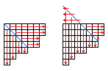
(a)                                               (b)

Figure 1: Frobenius notation for the ABJM case (a) and for the ABJ case (b). The same Young diagram $[\lambda_{1}\lambda_{2}\lambda_{3}\lambda_{4}\lambda_{5}\lambda_{6}\lambda_{7}]=[7766421]$ or $[\lambda^{\prime}_{1}\lambda^{\prime}_{2}\lambda^{\prime}_{3}\lambda^{\prime}_{4}\lambda^{\prime}_{5}\lambda^{\prime}_{6}\lambda^{\prime}_{7}]=[7655442]$ is expressed as $(a_{1}a_{2}a_{3}a_{4}|l_{1}l_{2}l_{3}l_{4})=(6532|6421)$ in the ABJM case while $(a_{1}a_{2}a_{3}|l_{1}l_{2}l_{3}l_{4}l_{5}l_{6})=(320|975421)$ in the ABJ case $(M=3)$. It is also convenient to regard the first three horizontal arrows in (b) as additional arm lengths $(-1,-2,-3)$.

2.1 Proof of the formula for the partition function

In this subsection, we shall present a proof for (2.3). Let us plug $x_{i}=e^{\mu_{i}}$ and $y_{a}=e^{\nu_{a}}$ or $x_{i}=e^{-\mu_{i}}$ and $y_{a}=e^{-\nu_{a}}$ into (2.14). Multiplying these two equations side by side, we find

$$(-1)^{\frac{1}{2}N_{1}(N_{1}-1)+\frac{1}{2}N_{2}(N_{2}-1)}\left(\frac{\prod_{i<j}2\sinh\frac{\mu_{i}-\mu_{j}}{2}\cdot\prod_{a<b}2\sinh\frac{\nu_{a}-\nu_{b}}{2}}{\prod_{i,a}2\cosh\frac{\mu_{i}-\nu_{a}}{2}}\right)^{2}$$

$$=\det\begin{pmatrix}({\bm{P}}(\mu_{i},\nu_{j}))_{\begin{subarray}{c}1\leq i\leq N_{1}\\ 1\leq j\leq N_{2}\end{subarray}}\\ ({E}_{M-p}(\nu_{j}))_{\begin{subarray}{c}1\leq p\leq M\\ 1\leq j\leq N_{2}\end{subarray}}\end{pmatrix}\det\begin{pmatrix}({\bm{Q}}(\nu_{j},\mu_{i}))_{\begin{subarray}{c}1\leq i\leq N_{1}\\ 1\leq j\leq N_{2}\end{subarray}}\\ ({E}_{-M+p-1}(\nu_{j}))_{\begin{subarray}{c}1\leq p\leq M\\ 1\leq j\leq N_{2}\end{subarray}}\end{pmatrix},$$ (2.16)

where ${\bm{Q}}$, ${\bm{P}}$ and ${E}$ are defined in (2.5). In order to evaluate the integration of the product (2.16) of two $N_{2}\times N_{2}$ determinants, we apply the formula (A.1) with $r=0$. Then we obtain

$$(-1)^{\frac{1}{2}N_{1}(N_{1}-1)+\frac{1}{2}N_{2}(N_{2}-1)}\frac{1}{N_{2}!}\int\prod_{a=1}^{N_{2}}\frac{d\nu_{a}}{2\pi}\ \left(\frac{\prod_{i<j}2\sinh\frac{\mu_{i}-\mu_{j}}{2}\cdot\prod_{a<b}2\sinh\frac{\nu_{a}-\nu_{b}}{2}}{\prod_{i,a}2\cosh\frac{\mu_{i}-\nu_{a}}{2}}\right)^{2}e^{-\frac{\mathtt{i}k}{4\pi}\sum_{a}\nu_{a}^{2}}$$

$$=\det\begin{pmatrix}(({\bm{P}}\circ{\bm{Q}})(\mu_{i},\mu_{j}))_{1\leq i,j\leq N_{1}}&(({\bm{P}}\circ{E}_{-M+q-1})(\mu_{i}))_{\begin{subarray}{c}1\leq i\leq N_{1}\\ 1\leq q\leq M\end{subarray}}\\ (({E}_{M-p}\circ{\bm{Q}})(\mu_{j}))_{\begin{subarray}{c}1\leq p\leq M\\ 1\leq j\leq N_{1}\end{subarray}}&({E}_{M-p}\circ{E}_{-M+q-1})_{1\leq p,q\leq M}\end{pmatrix},$$ (2.17)

where the explicit expression for each component in the determinant is given by

$$({\bm{P}}\circ{\bm{Q}})(\mu,\mu^{\prime}) =\int\frac{d\nu}{2\pi}{\bm{P}}(\mu,\nu){\bm{Q}}(\nu,\mu^{\prime})e^{-\frac{\mathtt{i}k}{4\pi}\nu^{2}}, ({\bm{P}}\circ{E}_{q})(\mu) =\int\frac{d\nu}{2\pi}{\bm{P}}(\mu,\nu){E}_{q}(\nu)e^{-\frac{\mathtt{i}k}{4\pi}\nu^{2}},$$

$$({E}_{p}\circ{\bm{Q}})(\mu) =\int\frac{d\nu}{2\pi}{E}_{p}(\nu){\bm{Q}}(\nu,\mu)e^{-\frac{\mathtt{i}k}{4\pi}\nu^{2}}, {E}_{p}\circ{E}_{q} =\int\frac{d\nu}{2\pi}{E}_{p}(\nu){E}_{q}(\nu)e^{-\frac{\mathtt{i}k}{4\pi}\nu^{2}}.$$ (2.18)

Therefore the grand partition function (2.2) becomes

$$\Xi_{k,M}(z) =\sum_{N=0}^{\infty}\frac{z^{N}}{N!}\int\prod_{i=1}^{N}e^{\frac{\mathtt{i}k}{4\pi}\mu_{i}^{2}}\frac{d\mu_{i}}{2\pi}\det\begin{pmatrix}(({\bm{P}}\circ{\bm{Q}})(\mu_{i},\mu_{j}))_{N\times N}&(({\bm{P}}\circ{E}_{-M+q-1})(\mu_{i}))_{N\times M}\\ (({E}_{M-p}\circ{\bm{Q}})(\mu_{j}))_{M\times N}&({E}_{M-p}\circ{E}_{-M+q-1})_{M\times M}\end{pmatrix},$$ (2.19)

which can be expressed as the Fredholm determinant $\operatorname{Det}$ of the form

$$\Xi_{k,M}(z)=\operatorname{Det}\begin{pmatrix}\mathbf{1}+z{\bm{P}}\circ{\bm{Q}}&z{\bm{P}}\circ{E}\\ {E}\circ{\bm{Q}}&{E}\circ{E}\end{pmatrix},$$ (2.20)

by appendix B. Using the formula

$$\operatorname{Det}\begin{pmatrix}A&B\\ C&D\end{pmatrix}=\operatorname{Det}A\cdot\operatorname{Det}(D-CA^{-1}B),$$ (2.21)

and simplifying the components by

$${E}_{p}\circ{E}_{q}-z{E}_{p}\circ{\bm{Q}}\circ\bigl{[}1+z{\bm{P}}\circ{\bm{Q}}\circ\bigr{]}^{-1}{\bm{P}}\circ{E}_{q}={E}_{p}\circ\bigl{[}1+z{\bm{Q}}\circ{\bm{P}}\circ\bigr{]}^{-1}{E}_{q},$$ (2.22)

we finally arrive at (2.3).

2.2 Proof of the formula for the half-BPS Wilson loop

In this subsection we shall present a proof for (2.10). The discussion is parallel to that of the previous subsection. From the formula due to Moens and Van der Jeugt [35], we have

$$s_{\lambda}((e^{\mu_{1}},\dots,e^{\mu_{N_{1}}})/(e^{\nu_{1}},\dots,e^{\nu_{N_{2}}}))$$

$$=(-1)^{r}\det\begin{pmatrix}({\bm{P}}(\mu_{i},\nu_{j}))_{\begin{subarray}{c}1\leq i\leq N_{1}\\ 1\leq j\leq N_{2}\end{subarray}}&({E}_{a_{q}}(\mu_{i}))_{\begin{subarray}{c}1\leq i\leq N_{1}\\ 1\leq q\leq r\end{subarray}}\\ ({E}_{l_{p}}(\nu_{j}))_{\begin{subarray}{c}1\leq p\leq M+r\\ 1\leq j\leq N_{2}\end{subarray}}&(0)_{(M+r)\times r}\end{pmatrix}\bigg{/}\det\begin{pmatrix}({\bm{P}}(\mu_{i},\nu_{j}))_{\begin{subarray}{c}1\leq i\leq N_{1}\\ 1\leq j\leq N_{2}\end{subarray}}\\ ({E}_{M-p}(\nu_{j}))_{\begin{subarray}{c}1\leq p\leq M\\ 1\leq j\leq N_{2}\end{subarray}}\end{pmatrix},$$ (2.23)

where $(a_{1}a_{2}\cdots a_{r}|l_{1}l_{2}\cdots l_{M+r})$ is the modified Frobenius notation of $\lambda$ given in (2.12). Combining this determinantal expression with (2.16), we have

$$(-1)^{\frac{1}{2}N_{1}(N_{1}-1)+\frac{1}{2}N_{2}(N_{2}-1)}s_{\lambda}((e^{\mu_{1}},\dots,e^{\mu_{N_{1}}})/(e^{\nu_{1}},\dots,e^{\nu_{N_{2}}}))$$

$$\hskip 170.71652pt\times\left(\frac{\prod_{i<j}2\sinh\frac{\mu_{i}-\mu_{j}}{2}\cdot\prod_{a<b}2\sinh\frac{\nu_{a}-\nu_{b}}{2}}{\prod_{i,a}2\cosh\frac{\mu_{i}-\nu_{a}}{2}}\right)^{2}$$

$$=(-1)^{r}\det\begin{pmatrix}({\bm{P}}(\mu_{i},\nu_{j}))_{\begin{subarray}{c}1\leq i\leq N_{1}\\ 1\leq j\leq N_{2}\end{subarray}}&({E}_{a_{q}}(\mu_{i}))_{\begin{subarray}{c}1\leq i\leq N_{1}\\ 1\leq q\leq r\end{subarray}}\\ ({E}_{l_{p}}(\nu_{j}))_{\begin{subarray}{c}1\leq p\leq M+r\\ 1\leq j\leq N_{2}\end{subarray}}&(0)_{(M+r)\times r}\end{pmatrix}\det\begin{pmatrix}({\bm{Q}}(\nu_{j},\mu_{i}))_{\begin{subarray}{c}1\leq i\leq N_{1}\\ 1\leq j\leq N_{2}\end{subarray}}\\ ({E}_{-M+p-1}(\nu_{j}))_{\begin{subarray}{c}1\leq p\leq M\\ 1\leq j\leq N_{2}\end{subarray}}\end{pmatrix}.$$ (2.24)

Integrating this with the formula (A.1), we see that

$$(-1)^{\frac{1}{2}N_{1}(N_{1}-1)+\frac{1}{2}N_{2}(N_{2}-1)}\frac{1}{N_{2}!}\int\prod_{a=1}^{N_{2}}e^{-\frac{\mathtt{i}k}{4\pi}\nu_{a}^{2}}\frac{d\nu_{a}}{2\pi}\left(\frac{\prod_{i<j}2\sinh\frac{\mu_{i}-\mu_{j}}{2}\cdot\prod_{a<b}2\sinh\frac{\nu_{a}-\nu_{b}}{2}}{\prod_{i,a}2\cosh\frac{\mu_{i}-\nu_{a}}{2}}\right)^{2}$$

$$\hskip 170.71652pt\times s_{\lambda}((e^{\mu_{1}},\dots,e^{\mu_{N_{1}}})/(e^{\nu_{1}},\dots,e^{\nu_{N_{2}}}))$$

$$=(-1)^{r}\det\begin{pmatrix}(({\bm{P}}\circ{\bm{Q}})(\mu_{i},\mu_{j}))_{\begin{subarray}{c}1\leq i\leq N_{1}\\ 1\leq j\leq N_{1}\end{subarray}}&(({\bm{P}}\circ{E}_{-M+q-1})(\mu_{i}))_{\begin{subarray}{c}1\leq i\leq N_{1}\\ 1\leq q\leq M\end{subarray}}&({E}_{a_{q}}(\mu_{i}))_{\begin{subarray}{c}1\leq i\leq N_{1}\\ 1\leq q\leq r\end{subarray}}\\ (({E}_{l_{p}}\circ{\bm{Q}})(\mu_{j}))_{\begin{subarray}{c}1\leq p\leq M+r\\ 1\leq j\leq N_{1}\end{subarray}}&({E}_{l_{p}}\circ{E}_{-M+q-1})_{\begin{subarray}{c}1\leq p\leq M+r\\ 1\leq q\leq M\end{subarray}}&(0)_{(M+r)\times r}\end{pmatrix}.$$ (2.25)

Now the definition (2.9) of $\langle s_{\lambda}\rangle_{k,M}^{\rm GC}(z)$ and appendix B give

$$\langle s_{\lambda}\rangle_{k,M}^{\rm GC}(z) =(-1)^{r}\sum_{N=0}^{\infty}\frac{z^{N}}{N!}\prod_{i=1}^{N}e^{\frac{\mathtt{i}k}{4\pi}\mu_{i}^{2}}\frac{d\mu_{i}}{2\pi}$$

$$\quad\times\det\begin{pmatrix}(({\bm{P}}\circ{\bm{Q}})(\mu_{i},\mu_{j}))_{N\times N}&({\bm{P}}\circ{E}_{-M+q-1}(\mu_{i}))_{N\times M}&({E}_{a_{q}}(\mu_{i}))_{N\times r}\\ (({E}_{l_{p}}\circ{\bm{Q}})(\mu_{j}))_{(M+r)\times N}&({E}_{l_{p}}\circ{E}_{-M+q-1})_{(M+r)\times M}&(0)_{(M+r)\times r}\end{pmatrix}$$

$$=(-1)^{r}\operatorname{Det}\begin{pmatrix}1+z{\bm{P}}\circ{\bm{Q}}&z{\bm{P}}\circ{E}&z{E}_{a}\\ {E}_{l}\circ{\bm{Q}}&{E}_{l}\circ{E}&0\end{pmatrix}.$$ (2.26)

Finally, using (2.21) and (2.22), we find

$$\frac{\langle s_{\lambda}\rangle_{k,M}^{\rm GC}(z)}{\Xi_{k,0}(z)}$$

$$=(-1)^{r}\operatorname{Det}\left[{E}_{l}\circ{E}-{E}_{l}\circ{\bm{Q}}\circ(1+z{\bm{P}}\circ{\bm{Q}}\circ)^{-1}z{\bm{P}}\circ{E}\ \bigm{|}\ -{E}_{l}\circ{\bm{Q}}\circ(1+z{\bm{P}}\circ{\bm{Q}}\circ)^{-1}z{E}_{a}\right]$$

$$=\operatorname{Det}\left[{E}_{l}\circ(1+z{\bm{Q}}\circ{\bm{P}}\circ)^{-1}{E}\ \bigm{|}\ z{E}_{l}\circ(1+z{\bm{Q}}\circ{\bm{P}}\circ)^{-1}{\bm{Q}}\circ{E}_{a}\right],$$ (2.27)

which is the desired formula (2.10). In the last determinant, the rows are determined by modified legs $l_{1},l_{2},\dots,l_{M+r}$, whereas the columns are determined by $(-M,\dots,-2,-1)$ and modified arms $a_{1},a_{2},\dots,a_{r}$.

3 Consistency with the previous works

In the subsequent sections, we shall use our Fermi gas formalism (2.3) to evaluate several values of the partition function and proceed to confirm our conjecture of the grand potential in (1.2). However, obviously only the values of the partition function at several coupling constants are not enough to fix the whole large $\mu$ expansion in (1.2). Hence, before starting our numerical studies, we shall first pause to study the consistency between our conjecture of the perturbative part and the worldsheet instanton part in (1.2) with the corresponding parts in the ’t Hooft expansion [6]. After fixing the worldsheet instanton contribution, we easily see that it diverges at some coupling constants. As in the case of the ABJM matrix model [8], since the matrix model is finite for any $(k,M)$ satisfying $0\leq M\leq k$ (at least $0\leq M\leq k/2$, as we shall see in the next section), the divergences in the worldsheet instantons have to be cancelled by the membrane instantons and their bound states. We shall see that, for this cancellation mechanism to work for $d_{k,M}^{(m)}$, we need to introduce the phase $(-1)^{M\ell}$ for $\mathaccent 869{b}_{k}^{(\ell)}$ and $\mathaccent 869{c}_{k}^{(\ell)}$ in (1.2).

3.1 Perturbative sum

The perturbative part of the grand potential in (1.2) implies that the perturbative sum of the partition function reads

$$Z^{\rm pert}_{k}(N,N+M)=e^{A_{k}}C_{k}^{-1/3}\operatorname{Ai}[C_{k}^{-1/3}(N-B_{k,M})].$$ (3.1)

The argument of the Airy function is proportional to

$$\frac{N-B_{k,M}}{k}=\hat{\lambda}-\frac{1}{3k^{2}}.$$ (3.2)

It was noted in [36, 6] that the renormalized ’t Hooft coupling constant

$$\hat{\lambda}=\frac{N}{k}-\frac{1}{24},$$ (3.3)

in the ABJM case has to be modified to

$$\hat{\lambda}=\frac{N_{1}+N_{2}}{2k}-\frac{(N_{1}-N_{2})^{2}}{2k^{2}}-\frac{1}{24},$$ (3.4)

in the ABJ case. We have changed $B_{k,0}$ into $B_{k,M}$ to take care of this modification.

3.2 Worldsheet instanton

Let us see the validity of our conjecture on the worldsheet instanton $d^{(m)}_{k,M}$. First note that the worldsheet instanton can be summarized into a multi-covering formula

$$J^{\rm WS}(\mu)=\sum_{g=0}^{\infty}\sum_{n,d_{1},d_{2}}n^{g}_{d_{1},d_{2}}\biggl{(}2\sin\frac{2\pi n}{k}\biggr{)}^{2g-2}\frac{(-e^{-\frac{4\mu}{k}}\beta^{-1})^{nd_{1}}(-e^{-\frac{4\mu}{k}}\beta)^{nd_{2}}}{n}.$$ (3.5)

This naturally corresponds to shifting the two Kahler parameters by $\pm 2\pi\mathtt{i}M/k$.

Next, we shall see that the expression of the worldsheet instanton (1.4) reproduces the genus-0 free energy of the matrix model [6]. As in [8], the first few worldsheet instanton terms of the free energy $F_{k,M}=\log Z_{k,M}$ with abbreviation $Z_{k,M}=Z_{k}(N,N+M)$ are given by

$$F^{{\rm WS}(1)}_{k,M} =Z^{{\rm WS}(1)}_{k,M},$$

$$F^{{\rm WS}(2)}_{k,M} =Z^{{\rm WS}(2)}_{k,M}-\frac{1}{2}(Z^{{\rm WS}(1)}_{k,M})^{2},$$ (3.6)

where the partition functions are

$$Z^{{\rm WS}(1)}_{k,M} =d^{(1)}_{k,M}\frac{\operatorname{Ai}[C_{k}^{-1/3}(N+\frac{4}{k}-B_{k,M})]}{\operatorname{Ai}[C_{k}^{-1/3}(N-B_{k,M})]},$$

$$Z^{{\rm WS}(2)}_{k,M} =\biggl{(}d^{(2)}_{k,M}+\frac{(d^{(1)}_{k,M})^{2}}{2}\biggr{)}\frac{\operatorname{Ai}[C_{k}^{-1/3}(N+\frac{8}{k}-B_{k,M})]}{\operatorname{Ai}[C_{k}^{-1/3}(N-B_{k,M})]},$$ (3.7)

and we have assumed that the worldsheet instantons are given by (1.4),

$$d^{(1)}_{k,M} =-\frac{n^{0}_{10}\beta^{-1}+n^{0}_{01}\beta}{4\sin^{2}\frac{2\pi}{k}},$$

$$d^{(2)}_{k,M} =\frac{n^{0}_{10}\beta^{-2}+n^{0}_{01}\beta^{2}}{8\sin^{2}\frac{4\pi}{k}}+\frac{n^{0}_{20}\beta^{-2}+n^{0}_{11}+n^{0}_{02}\beta^{2}}{4\sin^{2}\frac{2\pi}{k}}.$$ (3.8)

From the asymptotic form of the Airy function

$$\operatorname{Ai}[z]=\frac{e^{-\frac{2}{3}z^{3/2}}}{2\sqrt{\pi}z^{1/4}}\biggl{(}1-\frac{5}{48}z^{-3/2}+{\mathcal{O}}(z^{-3})\biggr{)},$$ (3.9)

we find

$$\frac{\operatorname{Ai}[C_{k}^{-1/3}(N+\frac{4m}{k}-B_{k,M})]}{\operatorname{Ai}[C_{k}^{-1/3}(N-B_{k,M})]}=e^{-2\pi\sqrt{2\hat{\lambda}}m}\biggl{(}1-\frac{2\sqrt{2}\pi m(m-\frac{1}{6})}{k^{2}\sqrt{\hat{\lambda}}}-\frac{m}{k^{2}\hat{\lambda}}+{\mathcal{O}}(k^{-4})\biggr{)}.$$ (3.10)

Hence, the free energy is given by

$$F^{{\rm WS}(1)}_{k,M} =e^{-2\pi\sqrt{2\hat{\lambda}}}\biggl{[}g_{s}^{-2}\frac{1}{4}(n^{0}_{10}\beta^{-1}+n^{0}_{01}\beta)+{\mathcal{O}}(g_{s}^{0})\biggr{]},$$

$$F^{{\rm WS}(2)}_{k,M} =e^{-4\pi\sqrt{2\hat{\lambda}}}\biggl{[}g_{s}^{-2}\biggl{(}-\frac{1}{32}(n^{0}_{10}\beta^{-2}+n^{0}_{01}\beta^{2})-\frac{1}{4}(n^{0}_{20}\beta^{-2}+n^{0}_{11}+n^{0}_{02}\beta^{2})$$

$$\qquad\qquad+\frac{1}{16}(n^{0}_{10}\beta^{-1}+n^{0}_{01}\beta)^{2}x\biggr{)}+{\mathcal{O}}(g_{s}^{0})\biggr{]},$$ (3.11)

with $x=1/(\pi\sqrt{2\hat{\lambda}})$.

After plugging the Gopakumar-Vafa invariants [37, 38],

$$n^{0}_{10}=n^{0}_{01}=-2,\quad n^{0}_{20}=n^{0}_{02}=0,\quad n^{0}_{11}=-4,$$ (3.12)

this reproduces the genus-0 free energy

$$F_{g=0} =\frac{4\pi^{3}\sqrt{2}}{3}\hat{\lambda}^{3/2}+\frac{2\pi^{3}\mathtt{i}}{3}\biggl{(}\frac{M}{k}\biggr{)}^{3}+{\rm const}$$

$$-\frac{1}{2}(\beta+\beta^{-1})e^{-2\pi\sqrt{2\hat{\lambda}}}+\biggl{(}\frac{1}{16}(\beta^{2}+16+\beta^{-2})+\frac{x}{4}(\beta+\beta^{-1})^{2}\biggr{)}e^{-4\pi\sqrt{2\hat{\lambda}}}+{\mathcal{O}}(e^{-6\pi\sqrt{2\hat{\lambda}}}),$$ (3.13)

which was found in subsection 5.3 of [6].

3.3 Cancellation mechanism

In the preceding subsections, we have presented a consistency check with previous studies for the perturbative part and the worldsheet instanton part of our conjecture (1.2). Note that these worldsheet instantons contain divergences at certain coupling constants. (See (3.8).) As in the case of the ABJM matrix model [8], since there should be no divergences in the matrix integration for $0\leq M\leq k$, the divergences have to be cancelled by the membrane instantons and the bound states. Corresponding to the extra phases from $\beta^{\pm 1}$ in $d_{k,M}^{(m)}$, we have found that the singularity of the worldsheet instanton (1.4) is cancelled if we introduce the extra sign factor $(-1)^{M\ell}$ in the membrane instantons. Namely, we have checked that the singularity in

$$d_{k,M}^{(m)}e^{-4m\mu_{\rm eff}/k}+(-1)^{M\ell}\bigl{(}\mathaccent 869{b}_{k}^{(\ell)}\mu_{\rm eff}+\mathaccent 869{c}_{k}^{(\ell)}\bigr{)}e^{-2\ell\mu_{\rm eff}},$$ (3.14)

at $k=2m/\ell$ is canceled for several values. The extra sign factor $(-1)^{M\ell}$ can also be understood by the shift of the Kahler parameters in the ABJ matrix model as pointed out below (3.5).

4 Phase factor

After the consistency check of the perturbative sum, the worldsheet instantons and the cancellation mechanism in the previous section, let us start to compute the grand partition function $\Xi_{k,M}(z)$ in (2.3). Since the grand partition function $\Xi_{k,0}(z)$ of the ABJM matrix model was studied carefully in our previous paper [8], we shall focus on the computation of the components of the matrix (2.4). After expanding in $z$, we find

$$H_{m,n}(z)=\sum_{N=0}^{\infty}(-z)^{N}H_{m,n}^{(N)},$$ (4.1)

where each term $H_{m,n}^{(N)}$ is simply given by a $2N+1$ multiple integration.

For $N=0$ we easily find ($\mathchar 1406\relax=2\pi k$)

$$H_{m,n}^{(0)}=\int\frac{dy}{\mathchar 1406\relax}e^{\frac{2\pi}{\mathchar 1406\relax}(m+\frac{1}{2})y}e^{-\frac{\mathtt{i}}{2\mathchar 1406\relax}y^{2}}e^{-\frac{2\pi}{\mathchar 1406\relax}(n+\frac{1}{2})y}=\frac{e^{-\frac{\pi\mathtt{i}}{4}}}{\sqrt{k}}e^{-\frac{2\pi\mathtt{i}}{2k}(m-n)^{2}},$$ (4.2)

while for $N\neq 0$ we find

$$H_{m,n}^{(N)} =\int\frac{dy_{0}}{\mathchar 1406\relax}\frac{dx_{1}}{\mathchar 1406\relax}\frac{dy_{1}}{\mathchar 1406\relax}\cdots\frac{dx_{N}}{\mathchar 1406\relax}\frac{dy_{N}}{\mathchar 1406\relax}e^{\frac{2\pi}{\mathchar 1406\relax}(m+\frac{1}{2})y_{0}}e^{-\frac{\mathtt{i}}{2\mathchar 1406\relax}y_{0}^{2}}\frac{1}{2\cosh\frac{y_{0}-x_{1}}{2k}}e^{\frac{\mathtt{i}}{2\mathchar 1406\relax}x_{1}^{2}}\frac{1}{2\cosh\frac{x_{1}-y_{1}}{2k}}$$

$$\quad\times e^{-\frac{\mathtt{i}}{2\mathchar 1406\relax}y_{1}^{2}}\cdots\frac{1}{2\cosh\frac{y_{N-1}-x_{N}}{2k}}e^{\frac{\mathtt{i}}{2\mathchar 1406\relax}x_{N}^{2}}\frac{1}{2\cosh\frac{x_{N}-y_{N}}{2k}}e^{-\frac{\mathtt{i}}{2\mathchar 1406\relax}y_{N}^{2}}e^{-\frac{2\pi}{\mathchar 1406\relax}(n+\frac{1}{2})y_{N}}.$$ (4.3)

Introducing the Fourier transformation,

$$\frac{1}{2\cosh\frac{y_{i-1}-x_{i}}{2k}} =\int\frac{dp_{i}}{2\pi}\frac{e^{-\mathtt{i}p_{i}(y_{i-1}-x_{i})/\mathchar 1406\relax}}{2\cosh\frac{p_{i}}{2}},$$

$$\frac{1}{2\cosh\frac{x_{i}-y_{i}}{2k}} =\int\frac{dq_{i}}{2\pi}\frac{e^{-\mathtt{i}q_{i}(x_{i}-y_{i})/\mathchar 1406\relax}}{2\cosh\frac{q_{i}}{2}},$$ (4.4)

and integrating over $y_{1},x_{1},\cdots,y_{N+1}$, we find

$$H_{m,n}^{(N)} =\frac{e^{-\frac{\pi\mathtt{i}}{4}}}{\sqrt{k}}e^{-\frac{2\pi\mathtt{i}}{2k}(m+\frac{1}{2})^{2}}e^{-\frac{2\pi\mathtt{i}}{2k}(n+\frac{1}{2})^{2}}\int\frac{dp_{1}dq_{1}}{2\pi\mathchar 1406\relax}\cdots\frac{dp_{N}dq_{N}}{2\pi\mathchar 1406\relax}$$

$$\quad e^{-\frac{1}{\mathchar 1406\relax}2\pi(m+\frac{1}{2})p_{1}}\frac{1}{2\cosh\frac{p_{1}}{2}}e^{\frac{\mathtt{i}}{\mathchar 1406\relax}p_{1}q_{1}}\frac{1}{2\cosh\frac{q_{1}}{2}}e^{-\frac{\mathtt{i}}{\mathchar 1406\relax}q_{1}p_{2}}\cdots e^{\frac{\mathtt{i}}{\mathchar 1406\relax}p_{N}q_{N}}\frac{1}{2\cosh\frac{q_{N}}{2}}e^{-\frac{1}{\mathchar 1406\relax}2\pi(n+\frac{1}{2})q_{N}}.$$ (4.5)

Using further the formulas

$$\int\frac{dp_{1}}{2\pi}e^{-\frac{1}{\mathchar 1406\relax}2\pi(m+\frac{1}{2})p_{1}}\frac{1}{2\cosh\frac{p_{1}}{2}}e^{\frac{\mathtt{i}}{\mathchar 1406\relax}p_{1}q_{1}} =\frac{1}{2\cosh\frac{q_{1}+2\pi\mathtt{i}(m+\frac{1}{2})}{2k}},$$

$$\int\frac{dp_{i}}{2\pi}\frac{e^{\frac{\mathtt{i}}{\mathchar 1406\relax}p_{i}(q_{i}-q_{i-1})}}{2\cosh\frac{p_{i}}{2}} =\frac{1}{2\cosh\frac{q_{i-1}-q_{i}}{2k}},\quad(i=2,3,\cdots,N-1)$$ (4.6)

to carry out the $p$-integrations, we finally arrive at the expression

$$H_{m,n}^{(N)} =\frac{e^{-\frac{\pi\mathtt{i}}{4}}}{\sqrt{k}}e^{-\frac{2\pi\mathtt{i}}{2k}(m+\frac{1}{2})^{2}}e^{-\frac{2\pi\mathtt{i}}{2k}(n+\frac{1}{2})^{2}}\int\frac{dq_{1}}{\mathchar 1406\relax}\frac{dq_{2}}{\mathchar 1406\relax}\cdots\frac{dq_{N}}{\mathchar 1406\relax}\frac{1}{2\cosh\frac{q_{1}+2\pi\mathtt{i}(m+\frac{1}{2})}{2k}}$$

$$\quad\times\frac{1}{2\cosh\frac{q_{1}}{2}}\frac{1}{2\cosh\frac{q_{1}-q_{2}}{2k}}\frac{1}{2\cosh\frac{q_{2}}{2}}\cdots\frac{1}{2\cosh\frac{q_{N-1}-q_{N}}{2k}}\frac{1}{2\cosh\frac{q_{N}}{2}}e^{-\frac{1}{k}(n+\frac{1}{2})q_{N}}.$$ (4.7)

As in the case of the Wilson loops, we can express $H_{m,n}^{(N)}$ ($N\neq 0$) as

$$H_{m,n}^{(N)}=\frac{e^{-\frac{\pi\mathtt{i}}{4}}}{\sqrt{k}}e^{-\frac{2\pi\mathtt{i}}{2k}(m+\frac{1}{2})^{2}}e^{-\frac{2\pi\mathtt{i}}{2k}(n+\frac{1}{2})^{2}}\int\frac{dx}{\mathchar 1406\relax}\frac{1}{2\cosh\frac{x+2\pi\mathtt{i}(m+\frac{1}{2})}{2k}}\frac{1}{2\cosh\frac{x}{2}}\phi_{n}^{(N-1)}(x),$$ (4.8)

where the functions $\phi_{n}^{(N)}(x)$ are defined by

$$\phi_{n}^{(N)}(x)=\sqrt{2\cosh\frac{x}{2}}\int\frac{dy}{\mathchar 1406\relax}\rho^{N}(x,y)\frac{e^{-\frac{1}{k}(n+\frac{1}{2})y}}{\sqrt{2\cosh\frac{y}{2}}},$$ (4.9)

with

$$\rho(x,y)=\frac{1}{\sqrt{2\cosh\frac{x}{2}}}\frac{1}{2\cosh\frac{x-y}{2k}}\frac{1}{\sqrt{2\cosh\frac{y}{2}}}.$$ (4.10)

In (4.9), the multiplication among the density matrices $\rho(x,y)$ is defined with a measure $1/\mathchar 1406\relax$,

$$\rho^{N}(x,y)=\int\frac{dz}{\mathchar 1406\relax}\,\rho(x,z)\,\rho^{N-1}(z,y).$$ (4.11)

The functions $\phi_{n}^{(N)}(x)$ can be determined recursively by

$$\phi_{n}^{(N)}(x)=\sqrt{2\cosh\frac{x}{2}}\int\frac{dy}{\mathchar 1406\relax}\rho(x,y)\frac{\phi_{n}^{(N-1)}(y)}{\sqrt{2\cosh\frac{y}{2}}},$$ (4.12)

with the initial condition $\phi_{n}^{(0)}(x)=e^{-\frac{1}{k}(n+\frac{1}{2})x}$.

Note that, in (4.8), the function $1/\cosh\frac{x+2\pi\mathtt{i}(m+\frac{1}{2})}{2k}$ has poles aligning on the imaginary axis. The pole with the smallest positive imaginary part is at $x=\pi\mathtt{i}(k-2(m+\frac{1}{2}))$ for $M$ in the range $0\leq M<(k+1)/2$ since $m$ runs from $0$ to $M-1$. Hence, for $M$ in this range, the relative position between the pole and the real axis is the same as the ABJM case $M=0$ and we can trust the formula (4.8) literally. However, for $(k+1)/2\leq M\leq k$ the above pole comes across the real axis and we need to deform the integration contour of (4.8), which is originally along the real axis, to the negative imaginary direction. This phenomenon and the contour prescription rule were already pointed out in [28]. In their work, they proposed this prescription by requiring the continuity at $M=(k+1)/2$ and the Seiberg duality. They also checked that this prescription gives the correct values of the partition function (2.1) for small $N$ and $k$. Our above analysis further pins down the origin of this deformation of the integration contour. The deformation comes from changing the integration variables from (4.3) to (4.8). For simplicity, hereafter, we shall often refer to the validity range as $0\leq M\leq k/2$ instead of $0\leq M<(k+1)/2$.

4.1 Phase factor

Unlike the case of the Wilson loops, the complex phase factor looks very non-trivial and needs to be studied separately. Using our Fermi gas formalism (2.3), we have found from numerical studies that the phase factor is given by a rather simple formula:

$$\frac{1}{2\pi}\arg Z_{k}(N,N+M)=\frac{1}{8}M(M-2)+\frac{1}{4}MN-\frac{1}{12k}(M^{3}-M).$$ (4.13)

We have checked this formula numerically for $N=0,1,2,3$. The results are depicted in figure 2. As noted in the above paragraph, our numerical studies are valid not only for $0\leq M\leq k/2$ but also slightly beyond $k/2$; $0<M<(k+1)/2$. In fact, we believe that our phase formula (4.13) is valid for the whole region of $0\leq M\leq k$ because we can show that this phase reproduces a phase factor appearing in the Seiberg duality

$$\frac{1}{2\pi}\arg\frac{Z_{k}(N,N+M)}{[Z_{k}(N,N+k-M)]^{*}}=\frac{k^{2}}{24}+\frac{1}{12}+\frac{k(N-1)}{4}$$ (4.14)

as was conjectured in [39] and further interpreted as a contact term anomaly in [40].

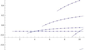
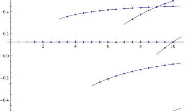
(a) $N=0$	(b) $N=1$
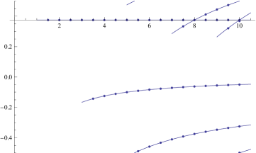
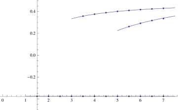
(c) $N=2$	(d) $N=3$

Figure 2: Numerical studies of the phase factor of the partition function. The horizontal axis denotes $k$ while the vertical axis shows the phase normalized by $2\pi$. Numerical data are depicted by points and our expectations (4.13) mod 1 are expressed by curves. Each picture corresponds to different values of $N$ and each curve in the picture starting from $k=2M-1$ corresponds different values of $M$.

5 Grand Potential

After studying the phase factor of the partition function in the previous section, let us turn to their absolute values and study the grand potential defined by these absolute values (1.1).

5.1 Grand potential at certain coupling constants

As was found in [15, 16, 8] the computation of the ABJM partition functions becomes particularly simple for $k=1,2,3,4,6$. Also, as we have seen in section 4, the formula (4.8) with integration along the real axis is literally valid only for $0\leq M\leq k/2$. Hence, we can compute various values of the partition function for

$$(k,M)=(2,1),(3,1),(4,1),(6,1),(4,2),(6,2),(6,3).$$ (5.1)

The results of their absolute values are summarized in figure 3. As discussed in [39], the case of $k/2\leq M\leq k$ is related to that of $0\leq M\leq k/2$ by the Seiberg duality.

$$|Z_{2}(0,1)|=\frac{1}{\sqrt{2}},\quad|Z_{2}(1,2)|=\frac{1}{4\sqrt{2}\pi},\quad|Z_{2}(2,3)|=\frac{\pi^{2}-8}{128\sqrt{2}\pi^{2}},$$

$$|Z_{2}(3,4)|=\frac{5\pi^{2}-48}{4608\sqrt{2}\pi^{3}},\quad|Z_{2}(4,5)|=\frac{81\pi^{4}-848\pi^{2}+480}{294912\sqrt{2}\pi^{4}},$$

$$|Z_{3}(0,1)|=\frac{1}{\sqrt{3}},\quad|Z_{3}(1,2)|=\frac{2-\sqrt{3}}{12},\quad|Z_{3}(2,3)|=\frac{-(9\sqrt{3}-14)\pi+3\sqrt{3}}{432\pi},$$

$$|Z_{3}(3,4)|=\frac{14\pi-18-15\sqrt{3}}{1728\pi},$$

$$|Z_{4}(0,1)|=\frac{1}{2},\quad|Z_{4}(1,2)|=\frac{\pi-2}{32\pi},$$

$$|Z_{4}(2,3)|=0.00003473909952494269119117566353230112859310233773233$$

$$\qquad 7261807934218890234955828380992634025931149937612,$$

$$|Z_{6}(0,1)|=\frac{1}{\sqrt{6}},\quad|Z_{6}(1,2)|=\frac{3\sqrt{3}-\pi}{108\sqrt{2}\pi},$$

$$|Z_{6}(2,3)|=3.76773027707758200049183186585155883429506373384028699$$

$$\qquad 96374213997516824024006754651401031813928511\times 10^{-6},$$

$$|Z_{6}(3,4)|=5.26914099452731795482041046853051131744637477848566664$$

$$\qquad 22916096253100787064300949345207528685791\times 10^{-10},$$

$$|Z_{4}(0,2)|=\frac{1}{2\sqrt{2}},\quad|Z_{4}(1,3)|=\frac{4-\pi}{32\sqrt{2}\pi},$$

$$|Z_{4}(2,4)|=0.00001506227428345380302357520499270222421841701033492$$

$$\qquad 362553063511451195968480813607610027807404966983,$$

$$|Z_{6}(0,2)|=\frac{1}{6},\quad|Z_{6}(1,3)|=\frac{7\pi-12\sqrt{3}}{432\pi},$$

$$|Z_{6}(2,4)|=4.77900663573206185466590506879892353173666149000261702$$

$$\qquad 495431896753514231026609667127826160173459\times 10^{-7},$$

$$|Z_{6}(0,3)|=\frac{1}{6\sqrt{2}},\quad|Z_{6}(1,4)|=\frac{45\sqrt{2}-8\sqrt{6}\pi}{1296\pi},$$

$$|Z_{6}(2,5)|=2.34333487780752843368477720747976341731283580616750538$$

$$\qquad 345879256373591282194222350629426352014176\times 10^{-7}.$$

Figure 3: Some exact or numerical values of partition functions.

Let us consider the grand potential defined with the absolute values of the partition function (1.1). Our strategy to determine the grand potential from the partition function is exactly the same as that of [8] and we shall explain only the key points here. Since the grand potential with the sum truncated at finite $N$ always contains some errors, it is known that fitting with the partition function itself gives a result with better accuracy. First we can compare the values found in figure 3 with the perturbative sum (3.1). This already shows a good concordance. For the $m$-th instanton effects, after subtracting the perturbative sum and the major instanton effects, we fit the partition function against the linear combinations of

$$(-\partial_{N})^{n}C_{k}^{-1/3}e^{A_{k}}{\rm Ai}\Bigl{[}C_{k}^{-1/3}\Bigl{(}N+\frac{4m}{k}-B_{k,M}\Bigr{)}\Bigr{]}.$$ (5.2)

Finally we reinterpret the result in terms of the grand potential. Our results are summarized in figure 4.

Compared with our study in [8, 18] we have much smaller number of exact values of the partition function. The lack of data causes quite significant numerical errors (about 1%). Nevertheless, since we have already known the rough structure of the instanton expansion, we can find the exact instanton coefficient without difficulty.

Note that the instanton coefficients of $(k,M)=(k,k/2)$ are similar to those of $(k,M)=(k,0)$ for even $k$ and those of $(k,M)=(6,1),(6,2)$ are similar to those of $(k,M)=(3,1)$. Due to this similarity, we have to confess that we only really fit the values of the partition function for $(k,M)=(3,1)$ and $(k,M)=(4,1)$ up to seven instantons. For other cases, after fitting for about three instantons, the patterns become clear and we can bring the results from the known ones and simply confirm the validity.

$$J^{\rm np}_{k=2,M=1} =\biggl{[}-\frac{4\mu^{2}+2\mu+1}{\pi^{2}}\biggr{]}e^{-2\mu}+\biggl{[}-\frac{52\mu^{2}+\mu+9/4}{2\pi^{2}}+2\biggr{]}e^{-4\mu}$$

$$\quad+\biggl{[}-\frac{736\mu^{2}-304\mu/3+154/9}{3\pi^{2}}+32\biggr{]}e^{-6\mu}$$

$$\quad+\biggl{[}-\frac{2701\mu^{2}-13949\mu/24+11291/192}{\pi^{2}}+466\biggr{]}e^{-8\mu}$$

$$\quad+\biggl{[}-\frac{161824\mu^{2}-634244\mu/15+285253/75}{5\pi^{2}}+6720\biggr{]}e^{-10\mu}$$

$$\quad+\biggl{[}-\frac{1227440\mu^{2}-5373044\mu/15+631257/20}{3\pi^{2}}+\frac{292064}{3}\biggr{]}e^{-12\mu}+{\mathcal{O}}(e^{-14\mu}),$$

$$J^{\rm np}_{k=3,M=1} =-\frac{2}{3}e^{-4\mu/3}-e^{-8\mu/3}+\biggl{[}\frac{4\mu^{2}+\mu+1/4}{3\pi^{2}}-\frac{34}{9}\biggr{]}e^{-4\mu}+\frac{25}{18}e^{-16\mu/3}+\frac{68}{15}e^{-20\mu/3}$$

$$\quad+\biggl{[}-\frac{52\mu^{2}+\mu/2+9/16}{6\pi^{2}}+\frac{296}{9}\biggr{]}e^{-8\mu}-\frac{1894}{189}e^{-28\mu/3}+{\mathcal{O}}(e^{-32\mu/3}),$$

$$J^{\rm np}_{k=4,M=1} =\biggl{[}\frac{4\mu^{2}+2\mu+1}{2\pi^{2}}-2\biggr{]}e^{-2\mu}+\biggl{[}-\frac{52\mu^{2}+\mu+9/4}{4\pi^{2}}+18\biggr{]}e^{-4\mu}$$

$$\quad+\biggl{[}\frac{736\mu^{2}-304\mu/3+154/9}{6\pi^{2}}-\frac{608}{3}\biggr{]}e^{-6\mu}+{\mathcal{O}}(e^{-8\mu}),$$

$$J^{\rm np}_{k=6,M=1} =\frac{2}{3}e^{-2\mu/3}-e^{-4\mu/3}+\biggl{[}-\frac{4\mu^{2}+2\mu+1}{3\pi^{2}}+\frac{34}{9}\biggr{]}e^{-2\mu}+\frac{25}{18}e^{-8\mu/3}-\frac{68}{15}e^{-10\mu/3}$$

$$\quad+\biggl{[}-\frac{52\mu^{2}+\mu+9/4}{6\pi^{2}}+\frac{296}{9}\biggr{]}e^{-4\mu}+\frac{1894}{189}e^{-14\mu/3}+{\mathcal{O}}(e^{-16\mu/3}),$$

$$J^{\rm np}_{k=4,M=2} =-e^{-\mu}+\biggl{[}-\frac{4\mu^{2}+2\mu+1}{2\pi^{2}}\biggr{]}e^{-2\mu}-\frac{16}{3}e^{-3\mu}+\biggl{[}-\frac{52\mu^{2}+\mu+9/4}{4\pi^{2}}+2\biggr{]}e^{-4\mu}$$

$$\quad-\frac{256}{5}e^{-5\mu}+\biggl{[}-\frac{736\mu^{2}-304\mu/3+154/9}{6\pi^{2}}+32\biggr{]}e^{-6\mu}-\frac{4096}{7}e^{-7\mu}+{\mathcal{O}}(e^{-8\mu}),$$

$$J^{\rm np}_{k=6,M=2} =-\frac{2}{3}e^{-\frac{2}{3}\mu}-e^{-\frac{4}{3}\mu}+\biggl{[}\frac{4\mu^{2}+2\mu+1}{3\pi^{2}}-\frac{34}{9}\biggr{]}e^{-2\mu}+\frac{25}{18}e^{-\frac{8}{3}\mu}+\frac{68}{15}e^{-\frac{10}{3}\mu}$$

$$\quad+\biggl{[}-\frac{52\mu^{2}+\mu+9/4}{6\pi^{2}}+\frac{296}{9}\biggr{]}e^{-4\mu}-\frac{1894}{189}e^{-\frac{14}{3}\mu}+{\mathcal{O}}(e^{-16\mu/3}),$$

$$J^{\rm np}_{k=6,M=3} =-\frac{4}{3}e^{-\frac{2}{3}\mu}-2e^{-\frac{4}{3}\mu}+\biggl{[}-\frac{4\mu^{2}+2\mu+1}{3\pi^{2}}-\frac{20}{9}\biggr{]}e^{-2\mu}-\frac{88}{9}e^{-\frac{8}{3}\mu}-\frac{108}{5}e^{-\frac{10}{3}\mu}$$

$$\quad+\biggl{[}-\frac{52\mu^{2}+\mu+9/4}{6\pi^{2}}-\frac{298}{9}\biggr{]}e^{-4\mu}-\frac{25208}{189}e^{-\frac{14}{3}\mu}+{\mathcal{O}}(e^{-16\mu/3}).$$

Figure 4: Grand potential obtained by fitting the exact or numerical values of partition function.

5.2 Grand potential for general coupling constants

Now let us compare the grand potential in figure 4 with a natural generalization of our instanton expansion in the ABJM matrix model. We first observe a good match for the $m$-th pure worldsheet instanton effects for $m<k/2$. Secondly, we find that we have to modify signs by the factor $(-1)^{M\ell}$ for the functions $a_{k}^{(\ell)}$, $\mathaccent 869{b}_{k}^{(\ell)}$, $\mathaccent 869{c}_{k}^{(\ell)}$ characterizing the membrane instantons. This is important not only for ensuring the cancellation of the divergences as we noted in subsection 3.3, but also for reproducing the correct coefficients of $\pi^{-2}$. Thirdly, we confirm that the prescription of introducing the sign factor $(-1)^{M\ell}$ reproduces correctly the bound states, where there are no pure membrane instanton effects.

As for the constant term in the membrane instanton, there is an ambiguity as long as it does not raise any singularities. There are two candidates for it: One is of course to take exactly the same constant term as in the ABJM case when expressed in terms of the chemical potential $\mu$. Another choice is to define $\mathaccent 869{c}_{k}^{(\ell)}$ by respecting the derivative relation. Namely, in the ABJM matrix model it was observed that, when the grand potential $J_{k}(\mu)$ is expressed in terms of the effective chemical potential $\mu_{\rm eff}$, the constant term is the derivative of the linear term (1.5). These two choices give different answers because of the change in $B_{k,M}$. Comparing these two candidates with our numerical results in figure 4, we have found that neither of them gives the correct answer. Instead, the difference with the latter one is always $k/M$ times bigger than the former one. From this observation, we can write down a closed form for our conjecture in (1.2). We have checked this conjecture up to seven worldsheet instantons and four membrane instantons.

Although we restrict our analysis to the case $0\leq M\leq k/2$, we believe our final conjecture (1.2) is valid for the whole region of $0\leq M\leq k$ because of the consistency with the Seiberg duality. Though the expression (1.2) does not look symmetric in the exchange between $M$ and $k-M$, if we pick up a pair of integers whose sum is $k$, we find two identical instanton expansion series after cancelling the divergences. We have checked this fact for all the pairs whose sums are $k=1,2,3,4,6$.

6 Discussions

In this paper we have proposed a Fermi gas formalism for the partition function and the half-BPS Wilson loop expectation values in the ABJ matrix models. Our formalism identifies the fractional branes in the ABJ theory as a certain type of Wilson loops in the ABJM theory. Hence, our formalism shares the same density matrix as that of the ABJM matrix model, which is suitable for the numerical studies. We have continued to study the exact or numerical values of the partition function using this formalism. Based on these values, we can determine the instanton expansion of the grand potential at some coupling constants $k=2,3,4,6$ and conjecture the expression (1.2) for general coupling constants.

Let us raise several points which need further clarifications.

The first one is the phase factor of our conjecture. As we have seen in figure 2, we have checked this conjecture for $N=0,1,2,3$ carefully. However when $N\geq 3$ the numerical errors become significant and it is difficult to continue the numerical studies with high accuracy for large $k$. It is desirable to study it more extensively.

The second one is the relation to the formalism of [28], which looks very different from ours. As pointed out very recently in [29] it was possible to rewrite the formalism of [28] into a mirror expression where the physical interpretation becomes clearer. We would like to see the exact relation between theirs and ours.

Thirdly, we have found an extra term in (1.2) proportional to the quantum mirror map $e_{k}^{(\ell)}$ [19]. We have very few data to identify its appearance and it would be great to check it also from the WKB expansion [14, 17], though we are not sure whether the restriction $0\leq M\leq k/2$ gives any difficulty in the WKB analysis. Furthermore, we cannot identify its origin in the refined topological strings or the triple sine functions as proposed in [19]. We hope to see its origin in these theories. It may be a key to understand the gravitational interpretation [42] of the membrane instantons.

The fourth one is about the Wilson loop in the ABJ theory. After seeing that there are only new terms appearing in the membrane instantons, we expect that the instanton expansion of the vacuum expectation values of the Wilson loop should be expressed similarly as that in the ABJM case [27]. However, we have not done any numerical studies to support it. Also, it is interesting to see how our study is related to other recent works on the ABJ Wilson loops [43, 44, 45].

Finally, one of the motivation to study the ABJ matrix model is its relation to the higher spin models. Since we have written down the grand potential explicitly, it is possible to take the limit proposed in [46]. We would like to see what lessons can be learned for the higher spin models.

Appendix A A useful determinantal formula

Lemma A.1.

Let $(\phi_{i})_{1\leq i\leq n+r}$ and $(\psi_{j})_{1\leq j\leq n}$ be functions on a measurable space and let $(\zeta_{iq})_{\begin{subarray}{c}1\leq i\leq n+r\\ 1\leq q\leq r\end{subarray}}$ be an array of constants. Then we have

$$\frac{1}{n!}\int\prod_{k=1}^{n}dx_{k}\cdot\det\left[(\phi_{i}(x_{k}))_{\begin{subarray}{c}1\leq i\leq n+r\\ 1\leq k\leq n\end{subarray}}\ (\zeta_{iq})_{\begin{subarray}{c}1\leq i\leq n+r\\ 1\leq q\leq r\end{subarray}}\right]\cdot\det(\psi_{j}(x_{k}))_{1\leq j,k\leq n}$$

$$=\det\left[(m_{ij})_{\begin{subarray}{c}1\leq i\leq n+r\\ 1\leq j\leq n\end{subarray}}\ (\zeta_{iq})_{\begin{subarray}{c}1\leq i\leq n+r\\ 1\leq q\leq r\end{subarray}}\right],$$ (A.1)

with $m_{ij}=\int dx\phi_{i}(x)\psi_{j}(x)$.

Proof.

Expand two determinants on the left hand side with respect to columns:

$$\frac{1}{n!}\int\prod_{k=1}^{n}dx_{k}\det\left[(\phi_{i}(x_{k}))_{\begin{subarray}{c}1\leq i\leq n+r\\ 1\leq k\leq n\end{subarray}}\ (\zeta_{iq})_{\begin{subarray}{c}1\leq i\leq n+r\\ 1\leq q\leq r\end{subarray}}\right]\cdot\det(\psi_{j}(x_{k}))_{1\leq j,k\leq n}$$

$$=\frac{1}{n!}\int\prod_{k=1}^{n}dx_{k}\sum_{\sigma\in S_{n+r}}\mathrm{sgn}(\sigma)\prod_{k=1}^{n}\phi_{\sigma(k)}(x_{k})\cdot\prod_{q=1}^{r}\zeta_{\sigma(n+q),q}\sum_{\tau\in S_{n}}\mathrm{sgn}(\tau)\prod_{k=1}^{n}\psi_{\tau(k)}(x_{k})$$

$$=\frac{1}{n!}\sum_{\sigma\in S_{n+r}}\mathrm{sgn}(\sigma)\prod_{q=1}^{r}\zeta_{\sigma(n+q),q}\cdot\sum_{\tau\in S_{n}}\mathrm{sgn}(\tau)\prod_{k=1}^{n}\int dx\phi_{\sigma(k)}(x)\psi_{\tau(k)}(x)$$

$$=\frac{1}{n!}\sum_{\tau\in S_{n}}\mathrm{sgn}(\tau)\sum_{\sigma\in S_{n+r}}\mathrm{sgn}(\sigma)\prod_{q=1}^{r}\zeta_{\sigma(n+q),q}\cdot\prod_{k=1}^{n}m_{\sigma(k),\tau(k)}$$

$$=\frac{1}{n!}\sum_{\tau\in S_{n}}\mathrm{sgn}(\tau)\det\left[(m_{i,\tau(j)})_{\begin{subarray}{c}1\leq i\leq n+r\\ 1\leq j\leq n\end{subarray}}\ (\zeta_{iq})_{\begin{subarray}{c}1\leq i\leq n+r\\ 1\leq q\leq r\end{subarray}}\right].$$ (A.2)

It follows from the alternating property for determinants that this equals to

$$\frac{1}{n!}\sum_{\tau\in S_{n}}\det\left[(m_{i,j})_{\begin{subarray}{c}1\leq i\leq n+r\\ 1\leq j\leq n\end{subarray}}\ (\zeta_{iq})_{\begin{subarray}{c}1\leq i\leq n+r\\ 1\leq q\leq r\end{subarray}}\right]=\det\left[(m_{i,j})_{\begin{subarray}{c}1\leq i\leq n+r\\ 1\leq j\leq n\end{subarray}}\ (\zeta_{iq})_{\begin{subarray}{c}1\leq i\leq n+r\\ 1\leq q\leq r\end{subarray}}\right].$$ (A.3)

∎

Appendix B Expansion of Fredholm determinant

Although we have used an infinite-dimensional version, we shall give a finite-dimensional version of the identity below. For a positive integer $n$, we let $[n]=\{1,2,\dots,n\}$.

Lemma B.1.

Let $N,L$ be non-negative integers. Let $A=(a_{ij})$, $B=(b_{iq})$, $C=(c_{pj})$, and $D=(d_{pq})$ be matrices of finite sizes $N\times N$, $N\times L$, $L\times N$, and $L\times L$, respectively. Let $\mathbf{1}^{\prime}_{NL}$ be the $(N+L)\times(N+L)$ diagonal matrix whose the first $N$ diagonal entries are $1$ and other entries are $0$. Then the following identity holds.

$$\det\left(\mathbf{1}^{\prime}_{NL}+\begin{pmatrix}A&B\\ C&D\end{pmatrix}\right)=\sum_{n=0}^{N}\frac{1}{n!}\sum_{k_{1},\dots,k_{n}=1}^{N}\det\begin{pmatrix}(a_{k_{i},k_{j}})_{1\leq i,j\leq n}&(b_{k_{i},q})_{1\leq i\leq n,1\leq q\leq L}\\ (c_{p,k_{j}})_{1\leq p\leq L,1\leq j\leq n}&D\end{pmatrix}.$$ (B.1)

Proof.

Put $\mathbf{A}=(\mathbf{a}_{ij})_{1\leq i,j\leq N+L}=\begin{pmatrix}A&B\\ C&D\end{pmatrix}$. Expanding the determinant with respect to rows, we have

$$\det(\mathbf{1}^{\prime}_{NL}+\mathbf{A})=\sum_{\sigma\in S_{N+L}}\mathrm{sgn}(\sigma)\prod_{i=1}^{N}(\delta_{i,\sigma(i)}+\mathbf{a}_{i,\sigma(i)})\times\prod_{p=1}^{L}\mathbf{a}_{N+p,\sigma(N+p)}.$$ (B.2)

Divide the product for $i$: for each $\sigma\in S_{N+L}$,

$$\prod_{i=1}^{N}(\delta_{i,\sigma(i)}+\mathbf{a}_{i,\sigma(i)})=\sum_{I\subset[N]}\prod_{i\in I}\mathbf{a}_{i,\sigma(i)}\times\prod_{i\in[N]\setminus I}\delta_{i,\sigma(i)}.$$ (B.3)

Here the product $\prod_{i\in[N]\setminus I}\delta_{i,\sigma(i)}$ vanishes unless $\sigma(i)=i$ for all $i\in[N]\setminus I$, i.e., unless the support $\mathrm{supp}(\sigma)$ of $\sigma$ is a subset of $I\cup\{N+1,\dots,N+L\}$. In that case, the permutation $\sigma$ can be seen as a permutation on $I\cup\{N+1,\dots,N+L\}$. Denoting by $S_{I\cup\{N+1,\dots,N+L\}}$ the permutation group consisting of such permutations,

$$\det(\mathbf{1}^{\prime}_{NL}+\mathbf{A})= \sum_{I\subset[N]}\sum_{\sigma\in S_{I\cup\{N+1,\dots,N+L\}}}\mathrm{sgn}(\sigma)\prod_{i\in I}\mathbf{a}_{i,\sigma(i)}\times\prod_{p=1}^{L}\mathbf{a}_{N+p,\sigma(N+p)}$$

$$= \sum_{I\subset[N]}\det\begin{pmatrix}(\mathbf{a}_{i,j})_{i,j\in I}&(\mathbf{a}_{i,N+q})_{i\in I,q\in[L]}\\ (\mathbf{a}_{N+p,j})_{p\in[L],j\in I}&(\mathbf{a}_{N+p,N+q})_{p,q\in[L]}\end{pmatrix}.$$ (B.4)

It is immediate to see that this identity presents the desired identity. ∎

References

• [1] O. Aharony, O. Bergman, D. L. Jafferis and J. Maldacena, “N=6 superconformal Chern-Simons-matter theories, M2-branes and their gravity duals,” JHEP 0810, 091 (2008) [arXiv:0806.1218 [hep-th]].
• [2] V. Pestun, “Localization of gauge theory on a four-sphere and supersymmetric Wilson loops,” Commun. Math. Phys.  313, 71 (2012) [arXiv:0712.2824 [hep-th]].
• [3] A. Kapustin, B. Willett and I. Yaakov, “Exact Results for Wilson Loops in Superconformal Chern-Simons Theories with Matter,” JHEP 1003, 089 (2010) [arXiv:0909.4559 [hep-th]].
• [4] D. L. Jafferis, “The Exact Superconformal R-Symmetry Extremizes Z,” JHEP 1205, 159 (2012) [arXiv:1012.3210 [hep-th]].
• [5] N. Hama, K. Hosomichi and S. Lee, “Notes on SUSY Gauge Theories on Three-Sphere,” JHEP 1103, 127 (2011) [arXiv:1012.3512 [hep-th]].
• [6] N. Drukker, M. Marino and P. Putrov, “From weak to strong coupling in ABJM theory,” Commun. Math. Phys.  306, 511 (2011) [arXiv:1007.3837 [hep-th]].
• [7] I. R. Klebanov and A. A. Tseytlin, “Entropy of near extremal black $p$-branes,” Nucl. Phys. B 475, 164 (1996) [hep-th/9604089].
• [8] Y. Hatsuda, S. Moriyama and K. Okuyama, “Instanton Effects in ABJM Theory from Fermi Gas Approach,” JHEP 1301, 158 (2013) [arXiv:1211.1251 [hep-th]].
• [9] H. Fuji, S. Hirano and S. Moriyama, “Summing Up All Genus Free Energy of ABJM Matrix Model,” JHEP 1108, 001 (2011) [arXiv:1106.4631 [hep-th]].
• [10] M. Hanada, M. Honda, Y. Honma, J. Nishimura, S. Shiba and Y. Yoshida, “Numerical studies of the ABJM theory for arbitrary N at arbitrary coupling constant,” JHEP 1205, 121 (2012) [arXiv:1202.5300 [hep-th]].
• [11] N. Drukker, M. Marino and P. Putrov, “Nonperturbative aspects of ABJM theory,” JHEP 1111, 141 (2011) [arXiv:1103.4844 [hep-th]].
• [12] C. P. Herzog, I. R. Klebanov, S. S. Pufu and T. Tesileanu, “Multi-Matrix Models and Tri-Sasaki Einstein Spaces,” Phys. Rev. D 83, 046001 (2011) [arXiv:1011.5487 [hep-th]].
• [13] K. Okuyama, “A Note on the Partition Function of ABJM theory on $S^{3}$,” Prog. Theor. Phys.  127, 229 (2012) [arXiv:1110.3555 [hep-th]].
• [14] M. Marino and P. Putrov, “ABJM theory as a Fermi gas,” J. Stat. Mech.  1203, P03001 (2012) [arXiv:1110.4066 [hep-th]].
• [15] Y. Hatsuda, S. Moriyama and K. Okuyama, “Exact Results on the ABJM Fermi Gas,” JHEP 1210, 020 (2012) [arXiv:1207.4283 [hep-th]].
• [16] P. Putrov and M. Yamazaki, “Exact ABJM Partition Function from TBA,” Mod. Phys. Lett. A 27, 1250200 (2012) [arXiv:1207.5066 [hep-th]].
• [17] F. Calvo and M. Marino, “Membrane instantons from a semiclassical TBA,” JHEP 1305, 006 (2013) [arXiv:1212.5118 [hep-th]].
• [18] Y. Hatsuda, S. Moriyama and K. Okuyama, “Instanton Bound States in ABJM Theory,” JHEP 1305, 054 (2013) [arXiv:1301.5184 [hep-th]].
• [19] Y. Hatsuda, M. Marino, S. Moriyama and K. Okuyama, “Non-perturbative effects and the refined topological string,” arXiv:1306.1734 [hep-th].
• [20] A. Mironov and A. Morozov, “Nekrasov Functions and Exact Bohr-Zommerfeld Integrals,” JHEP 1004, 040 (2010) [arXiv:0910.5670 [hep-th]].
• [21] A. Mironov and A. Morozov, “Nekrasov Functions from Exact BS Periods: The Case of SU(N),” J. Phys. A 43, 195401 (2010) [arXiv:0911.2396 [hep-th]].
• [22] M. Aganagic, M. C. N. Cheng, R. Dijkgraaf, D. Krefl and C. Vafa, “Quantum Geometry of Refined Topological Strings,” JHEP 1211, 019 (2012) [arXiv:1105.0630 [hep-th]].
• [23] O. Aharony, O. Bergman and D. L. Jafferis, “Fractional M2-branes,” JHEP 0811, 043 (2008) [arXiv:0807.4924 [hep-th]].
• [24] N. Drukker and D. Trancanelli, “A Supermatrix model for N=6 super Chern-Simons-matter theory,” JHEP 1002, 058 (2010) [arXiv:0912.3006 [hep-th]].
• [25] M. Marino and P. Putrov, “Exact Results in ABJM Theory from Topological Strings,” JHEP 1006, 011 (2010) [arXiv:0912.3074 [hep-th]].
• [26] J. Kallen and M. Marino, “Instanton effects and quantum spectral curves,” arXiv:1308.6485 [hep-th].
• [27] Y. Hatsuda, M. Honda, S. Moriyama and K. Okuyama, “ABJM Wilson Loops in Arbitrary Representations,” arXiv:1306.4297 [hep-th].
• [28] H. Awata, S. Hirano and M. Shigemori, “The Partition Function of ABJ Theory,” arXiv:1212.2966.
• [29] M. Honda, “Direct derivation of ‘mirror’ ABJ partition function,” arXiv:1310.3126 [hep-th].
• [30] J. McGreevy, L. Susskind and N. Toumbas, “Invasion of the giant gravitons from Anti-de Sitter space,” JHEP 0006, 008 (2000) [hep-th/0003075].
• [31] A. Borodin, G. Olshanski, E. Strahov, “Giambelli compatible point processes,” Advances in Applied Mathematics 37.2, 209-248 (2006), [arXiv:math-ph/0505021].
• [32] A. Klemm, M. Marino, M. Schiereck and M. Soroush, “ABJM Wilson loops in the Fermi gas approach,” arXiv:1207.0611 [hep-th].
• [33] A. Grassi, J. Kallen and M. Marino, “The topological open string wavefunction,” arXiv:1304.6097 [hep-th].
• [34] E. L. Basor and P. J. Forrester, “Formulas for the evaluation of Toeplitz determinants with rational generating functions,” Mathematische Nachrichten 170.1, 5-18 (1994).
• [35] E. M. Moens and J. Van der Jeugt, “A determinantal formula for supersymmetric Schur polynomials”, Journal of Algebraic Combinatorics 17.3 (2003) 283-307.
• [36] O. Aharony, A. Hashimoto, S. Hirano and P. Ouyang, “D-brane Charges in Gravitational Duals of 2+1 Dimensional Gauge Theories and Duality Cascades,” JHEP 1001, 072 (2010) [arXiv:0906.2390 [hep-th]].
• [37] R. Gopakumar and C. Vafa, “M theory and topological strings. 1.,” hep-th/9809187.
• [38] M. Aganagic, M. Marino and C. Vafa, “All loop topological string amplitudes from Chern-Simons theory,” Commun. Math. Phys.  247, 467 (2004) [hep-th/0206164].
• [39] A. Kapustin, B. Willett and I. Yaakov, “Tests of Seiberg-like Duality in Three Dimensions,” arXiv:1012.4021 [hep-th].
• [40] C. Closset, T. T. Dumitrescu, G. Festuccia, Z. Komargodski and N. Seiberg, “Comments on Chern-Simons Contact Terms in Three Dimensions,” JHEP 1209, 091 (2012) [arXiv:1206.5218 [hep-th]].
• [41] M. Shigemori, unpublished notes.
• [42] S. Bhattacharyya, A. Grassi, M. Marino and A. Sen, “A One-Loop Test of Quantum Supergravity,” arXiv:1210.6057 [hep-th].
• [43] V. Cardinali, L. Griguolo, G. Martelloni and D. Seminara, “New supersymmetric Wilson loops in ABJ(M) theories,” Phys. Lett. B 718, 615 (2012) [arXiv:1209.4032 [hep-th]].
• [44] M. Bianchi, G. Giribet, M. Leoni and S. Penati, “The 1/2 BPS Wilson loop in ABJ(M) at two loops: The details,” arXiv:1307.0786 [hep-th].
• [45] L. Griguolo, G. Martelloni, M. Poggi and D. Seminara, “Perturbative evaluation of circular 1/2 BPS Wilson loops in $\mathcal{N}=6$ Super Chern-Simons theories,” JHEP 1309, 157 (2013) [arXiv:1307.0787 [hep-th]].
• [46] C. -M. Chang, S. Minwalla, T. Sharma and X. Yin, “ABJ Triality: from Higher Spin Fields to Strings,” J. Phys. A 46, 214009 (2013) [arXiv:1207.4485 [hep-th]].