A no-boundary proposal for braneworld perturbations

Abstract

We propose a novel approach to the problem of cosmological perturbations in a braneworld model with induced gravity, which leads to a closed system of equations on the brane. We focus on a spatially closed brane that bounds the interior four-ball of the bulk space. The background cosmological evolution on the brane is now described by the normal branch, and the boundary conditions in the bulk become the regularity conditions for the metric everywhere inside the four-ball. In this approach, there is no spatial infinity or any other boundary in the bulk space since the spatial section is compact, hence, we term this setup as a no-boundary proposal. Assuming that the bulk cosmological constant is absent and employing the Mukohyama master variable, we argue that the effects of nonlocality on brane perturbations may be ignored if the brane is marginally closed. In this case, there arises a relation that closes the system of equations for perturbations on the brane. Perturbations of pressureless matter and dark radiation can now be described by a system of coupled second-order differential equations. Remarkably, this system can be exactly solved in the matter-dominated and de Sitter regimes. In this case, apart from the usual growing and decaying modes, we find two additional modes that behave monotonically on super-Hubble spatial scales and exhibit rapid oscillations with decaying amplitude on sub-Hubble spatial scales.

I Introduction

In the braneworld paradigm Maartens:2010ar , our observable universe is a four-dimensional hypersurface (the “brane”) embedded in a higher-dimensional spacetime (the “bulk”) with Standard-Model particles and fields trapped on the brane. In the most popular cosmological models, there is only one extra dimension, and the brane is either a boundary or is embedded into a five-dimensional bulk space-time. From the four-dimensional viewpoint, this can be regarded as a modification of gravity. In one of its popular versions, the Randall–Sundrum (RS) model RS , general relativity (and the inverse square law) is modified due to extra-dimensional effects on relatively small spatial scales. Apart from interesting high-energy implications of this model, it was shown to be potentially capable of explaining the observations of the galactic rotation curves and X-ray profiles of galactic clusters without invoking the notion of dark matter Rotation curves .

In another version of the braneworld paradigm, first proposed by Arkani-Hamed, Dimopoulos and Dvali ArkaniHamed:1998rs and subsequently developed by Dvali, Gabadadze and Porrati DGP (the DGP model), gravity is modified on large spatial scales. This model is based on the inclusion of the Hilbert–Einstein term in the action for the brane (so-called induced gravity), and, because of this, has two branches of cosmological solutions. The ‘self-accelerating’ branch can model cosmology with late-time acceleration without cosmological constants either in the bulk or on the brane, while the ‘normal’ branch requires at least a brane tension to accelerate the expansion. Subsequent analysis has revealed a serious stability issue of the self-accelerating branch of the DGP model — the so-called ghost instability Ghosts . This leaves the normal branch, perhaps, as the only physically viable solution, consistent with the current observation of cosmological acceleration. A general braneworld model containing the induced gravity term as well as cosmological constants in the bulk and on the brane, was first proposed and studied in Collins:2000yb ; Shtanov:2000vr ; Deffayet:2000uy . In describing the late-time cosmological acceleration on the normal branch, this model exhibits a number of interesting generic features, including the possibility of superacceleration (supernegative, or phantom-like, effective equation of state of dark energy $w_{\rm eff}\leq-1$) Sahni:2002dx ; Lue:2004za . It is interesting that a phantom-like equation of state arises in the normal branch without the development of a ‘Big-rip’ future singularity. Such an effective equation of state appears to be consistent with the most recent set of observations of type Ia supernovae combined with other data sets Rest:2013bya . Such a braneworld also admits the possibility of cosmological loitering even in a spatially flat universe Sahni:2004fb , and the property of cosmic mimicry, wherein a low-density braneworld shares the precise expansion history of $\Lambda$CDM Sahni:2005mc ; for a brief review see Sahni:review . This braneworld model can also be used to address astrophysical observations of dark matter in galaxies Viznyuk:2007ft .

The theory of structure formation, temperature anisotropy of the cosmic microwave background (CMB) and other issues that form the basis of experimental tests of any cosmological model require the knowledge of the evolution of cosmological perturbations. Developing the theory of cosmological perturbations in the braneworld context is a long-standing problem. The existence of an extra dimension requires taking into account the corresponding dynamical degrees of freedom and the specification of the boundary conditions in the bulk space. In the case of a spatially flat brane, the extra dimension is noncompact, and one has to deal with its spatial infinity. The main difficulty, in this case, is the presence of the bulk gravitational effects which lead to the non-locality of the resulting equations on the brane. In spite of the analytical complexity of the problem, considerable progress has been made in this direction over the last few years. Based on a very convenient Mukohyama master variable and master equation Mukohyama:2000ui ; Mukohyama:2001yp , interesting results were presented in Deffayet:2002fn ; Deffayet:2004xg ; Koyama:2005kd ; Koyama:2006ef ; Sawicki:2006jj ; Song:2007wd ; Seahra:2010fj . However, all analytical results (of which we are aware) are based on some kind of simplifying assumptions or approximations which are taken for granted. Thus, the well-known quasi-static (QS) approximation introduced by Koyama and Maartens Koyama:2005kd (for an extension into the non-linear regime, see non-linear ) is based on the assumption of slow temporal evolution of all quantities on sub-Hubble spatial scales, as compared to spatial gradients. Another approximation — the dynamical scaling (DS) ansatz, proposed by Sawicki et al. Sawicki:2006jj ; Song:2007wd — assumes that perturbations evolve as a power of the scale factor with time-varying index. Both approximations were further analyzed in Seahra:2010fj . A complete system of equations in the bulk and on the brane were solved numerically in the framework of the RS Cardoso:2007zh and DGP Cardoso:2007xc braneworld models.

Notwithstanding the partial success of approximate methods and numerical integration schemes, the problem of cosmological perturbations on the brane cannot be viewed as having been successfully solved without either a justification of the introduced approximations or an analytical solution. In this work, we propose a new approach to the issue of boundary conditions in the bulk which permits one to obtain a closed system of equations for scalar cosmological perturbations on a (marginally) closed brane without any simplifying assumptions (aside from assuming a small spatial curvature for the brane).

In the case of a spatially flat brane, the ‘standard’ method of setting boundary conditions on the past Cauchy horizon does not guarantee the absence of a singularity in the whole of the bulk space (for a discussion of this problem, see Shtanov:2007dh ). In the present paper, we consider a spatially closed brane, which is a boundary of the four-ball of the bulk space. (Alternatively, one can picture the spatially closed brane as embedded in the bulk with $Z_{2}$ symmetry of reflection with respect to the brane; in this case, there are two identical bulk spaces with four-ball topology on the two sides of the brane.) This configuration gives the normal branch of the theory and describes the model originally suggested in Shtanov:2000vr . There is no spatial infinity (or another boundary), and the boundary conditions in the bulk become natural and simple: the metric is required to be regular everywhere inside of the (evolving) four-ball bounded by the brane (see Fig. 1). In this regard, we call this setup a no-boundary proposal. In the simplest case where the unperturbed bulk space is flat (the bulk cosmological constant is equal to zero), we succeed in deriving a closed approximate system for scalar perturbations on the brane and find some exact analytical solutions.

The most important qualitative result of this investigation is that, apart from the usual monotonic growing and decaying modes for scalar-type perturbations, we find another two set of modes which behave in an oscillatory fashion with a slowly decaying amplitude.

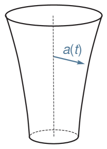
Figure 1: The spatially closed brane has a three-sphere ($S^{3}$) topology and bounds a four-ball in the bulk space. The expansion factor, $a(t)$, of the brane corresponds to the radial coordinate of the bulk space, as shown in this figure and discussed in greater detail in Sec. IV.

Our paper is organized as follows. In the next section, we introduce the braneworld equations and discuss their (unperturbed) cosmological solutions. In Sec. III, we present the system of equations describing scalar cosmological perturbations on the brane. This system is not closed because the evolution equation for the anisotropic stress of the bulk projection (the so-called Weyl fluid, or dark radiation) is missing. The anisotropic stress of the Weyl fluid is then expressed through the Mukohyama master variable in Sec. IV for the case of a spatially closed brane which bounds the bulk space. In this case, a general solution for the master variable can be found. In Sec. V, we prove that the effects of nonlocality may be ignored if the brane is marginally closed, and obtain a closed system of second-order differential equations describing the perturbations of pressureless matter and the Weyl fluid in this case. Some exact solutions of these equations are presented in Sec. VI. The results of our work are summarized in Sec. VII.

II Background cosmological evolution

We start from the generic form of the braneworld action:

$$S=M^{3}\left[\int_{\rm bulk}\left({\cal R}-2\Lambda\right)-2\int_{\rm brane}K\right]+\int_{\rm brane}\left(m^{2}R-2\sigma\right)+\int_{\rm brane}L\left(g_{\mu\nu},\phi\right)\,,$$ (1)

where ${\cal R}$ is the scalar curvature of the five-dimensional metric $g_{AB}$, and $R$ is the scalar curvature corresponding to the induced metric $g_{\mu\nu}$ on the brane. The symbol $L\left(g_{\mu\nu},\phi\right)$ denotes the Lagrangian density of the four-dimensional matter fields $\phi$ whose dynamics is restricted to the brane so that they interact only with the induced metric $g_{\mu\nu}$. The quantity $K$ is the trace of the symmetric tensor of extrinsic curvature of the brane. All integrations over the bulk and brane are taken with the corresponding natural volume elements. The universal constants $M$ and $m$ play the role of the five-dimensional and four-dimensional Planck masses, respectively. The symbol $\Lambda$ denotes the bulk cosmological constant, and $\sigma$ is the brane tension.

The actions of the RS RS and DGP DGP braneworld models are special cases of (1). The action of the RS braneworld is obtained after setting $m=0$ in (1), whereas neglecting $\Lambda$ and $\sigma$ leads to the DGP model. General relativity with $1/m^{2}$ playing the role of the gravitational constant can also be formally obtained from (1) after setting $M=0$.

The action (1) leads to the Einstein equation with a cosmological constant in the bulk,

$${\cal G}_{AB}+\Lambda g_{AB}=0\,,$$ (2)

and the following effective equation on the brane Shiromizu:1999wj ; Sahni:2005mc :

$$G_{\mu\nu}+\left(\frac{\Lambda_{\rm RS}}{{b}+1}\right)g_{\mu\nu}=\left(\frac{{b}}{{b}+1}\right)\frac{1}{m^{2}}\,T_{\mu\nu}+\left(\frac{1}{{b}+1}\right)\left[\frac{1}{M^{6}}Q_{\mu\nu}-{\cal C}_{\mu\nu}\right]\,,$$ (3)

where

$${b}=k\ell\,,\qquad k=\frac{\sigma}{3M^{3}}\,,\qquad\ell=\frac{2m^{2}}{M^{3}}\,,\qquad\Lambda_{\rm RS}=\frac{\Lambda}{2}+\frac{\sigma^{2}}{3M^{6}}$$ (4)

are convenient parameters to describe the braneworld model, and

$$Q_{\mu\nu}=\frac{1}{3}EE_{\mu\nu}-E_{\mu\lambda}E^{\lambda}{}_{\nu}+\frac{1}{2}\left(E_{\rho\lambda}E^{\rho\lambda}-\frac{1}{3}E^{2}\right)g_{\mu\nu}\,,$$ (5)

$$E_{\mu\nu}\equiv m^{2}G_{\mu\nu}-T_{\mu\nu}\,.$$ (6)

Gravitational dynamics on the brane is not closed because of the presence of the symmetric traceless tensor ${\cal C}_{\mu\nu}$ in (3), which is the projection of the five-dimensional Weyl tensor from the bulk onto the brane. The tensor ${\cal C}_{\mu\nu}$ is not freely specifiable on the brane, but is related to the tensor $Q_{\mu\nu}$ through the conservation equation

$$\nabla^{\mu}\left(Q_{\mu\nu}-M^{6}{\cal C}_{\mu\nu}\right)=0\,,$$ (7)

which is a consequence of the Bianchi identity applied to (3) and the law of stress–energy conservation for matter:

$$\nabla^{\mu}T_{\mu\nu}=0\,.$$ (8)

Here, $\nabla_{\mu}$ denotes the derivative on the brane compatible with the induced metric on the brane.

The cosmological evolution of the Friedmann–Robertson–Walker (FRW) braneworld model

$$ds^{2}=-dt^{2}+a^{2}(t)\gamma_{ij}dx^{i}dx^{j}\,$$ (9)

can be obtained from (3) with the following result Collins:2000yb ; Shtanov:2000vr ; Deffayet:2000uy ; Sahni:2002dx :

$$H^{2}+{\kappa\over a^{2}}={\rho+\sigma\over 3m^{2}}+{2\over\ell^{2}}\left[1\pm\sqrt{1+\ell^{2}\left({\rho+\sigma\over 3m^{2}}-{\Lambda\over 6}-{C\over a^{4}}\right)}\right]\,.$$ (10)

Here, $H\equiv\dot{a}/a$ is the Hubble parameter, $\rho=\rho(t)$ is the energy density of matter on the brane and $C$ is a constant resulting from the presence of the symmetric traceless tensor ${\cal C}_{\mu\nu}$ in the field equations (3). The parameter $\kappa=0,\pm 1$ corresponds to different spatial geometries of the maximally symmetric spatial metric $\gamma_{ij}$.

The $\pm$ sign in equation (10) reflects the two different ways in which the bulk can be bounded by the brane Deffayet:2000uy , resulting in two different branches of solutions. These are usually called the normal branch ($-$ sign) and the self-accelerating branch (+ sign).

III Scalar cosmological perturbations: combined system of equations on the brane

The scalar cosmological perturbations of the induced metric on the brane are most conveniently described by the relativistic potentials $\Phi$ and $\Psi$ in the longitudinal gauge:

$$ds^{2}=-(1+2\Phi)dt^{2}+a^{2}(1-2\Psi)\gamma_{ij}dx^{i}dx^{j}\,.$$ (11)

The components of the linearly perturbed stress–energy tensor of matter in these coordinates are defined as follows:

$$\delta T^{\mu}{}_{\nu}=\left(\begin{array}[]{cc}\displaystyle-\delta\rho\,,&\displaystyle-\nabla_{i}v\vskip 6.0pt plus 2.0pt minus 2.0pt\\ \displaystyle{\nabla^{i}v\over a^{2}}\,,&\displaystyle\delta p\,\delta^{i}{}_{j}+\frac{\zeta^{i}{}_{j}}{a^{2}}\end{array}\right)\,,$$ (12)

where $\delta\rho$, $\delta p$, $v$, and $\zeta_{ij}=\left(\nabla_{i}\nabla_{j}-\frac{1}{3}\gamma_{ij}\nabla^{2}\right)\zeta$ describe the scalar perturbations.

Similarly, we introduce the scalar perturbations $\delta\rho_{\cal C}$, $v_{\cal C}$, and $\delta\pi_{\cal C}$ of the tensor ${\cal C}_{\mu\nu}$:

$$m^{2}\delta{\cal C}^{\mu}{}_{\nu}=\left(\begin{array}[]{cc}\displaystyle-\delta\rho_{\cal C}\,,&\displaystyle-\nabla_{i}v_{\cal C}\vskip 6.0pt plus 2.0pt minus 2.0pt\\ \displaystyle{\nabla^{i}v_{\cal C}\over a^{2}}\,,&\displaystyle{\delta\rho_{\cal C}\over 3}\delta^{i}{}_{j}+{\delta\pi^{i}{}_{j}\over a^{2}}\end{array}\right)\,,$$ (13)

where $\delta\pi_{ij}=\left(\nabla_{i}\nabla_{j}-\frac{1}{3}\gamma_{ij}\nabla^{2}\right)\delta\pi_{\cal C}$.

We call $v$ and $v_{\cal C}$ the momentum potentials for matter and dark radiation, respectively, $\delta\rho$ and $\delta\rho_{\cal C}$ are their energy density perturbations, and $\zeta$ and $\delta\pi_{\cal C}$ are the scalar potentials for their anisotropic stresses.

Using this notation, one can derive a complete system of equations that describe the evolution of scalar cosmological perturbations on the brane (for details of the derivation see Shtanov:2007dh ; Viznyuk:2012oda ):

$${1\over a^{2}}\left(\nabla^{2}+3\kappa\right)\Psi=\left(1+{2\over\beta}\right){\rho\,\Delta\over 2m^{2}}+{\left(\delta\rho_{\cal C}+3Hv_{\cal C}\right)\over m^{2}\beta}\,,$$ (14)

$$m^{2}\beta\left(\dot{\Psi}+H\Phi\right)=\left(1+{\beta\over 2}\right)v+v_{\cal C}\,,$$ (15)

$$\ddot{\Psi} + 3(1+\gamma)H\dot{\Psi}+H\dot{\Phi}+\left[2\dot{H}+3H^{2}(1+\gamma)\right]\Phi\,-$$ (16)

$$- {\gamma\over a^{2}}\nabla^{2}\Psi-{\kappa(1+3\gamma)\over a^{2}}\Psi+{1\over 3a^{2}}\nabla^{2}(\Phi-\Psi)\,=$$

$$= \displaystyle-\left(\gamma+{2\over 3\beta}\right){\delta\rho\over 2m^{2}}+\left(1+{2\over\beta}\right){\delta p\over 2m^{2}}\,,$$

$$\frac{\delta\pi_{\cal C}}{m^{2}}=-\frac{\beta(3\gamma+1)}{4}\left(\Phi-\Psi+{\zeta\over m^{2}}\right)-\frac{\zeta}{m^{2}}\,,$$ (17)

$$\delta\dot{\rho}+3H(\delta\rho+\delta p)={1\over a^{2}}\nabla^{2}v+3(\rho+p)\dot{\Psi}\,,$$ (18)

$$\dot{v}+3Hv=\delta p+(\rho+p)\Phi+{2\over 3a^{2}}\left(\nabla^{2}+3\kappa\right)\zeta\,,$$ (19)

$$\delta\dot{\rho}_{\cal C}+4H\delta\rho_{\cal C}={1\over a^{2}}\nabla^{2}v_{\cal C}-{12m^{2}C\over a^{4}}\dot{\Psi}\,,$$ (20)

$$\dot{v}_{\cal C} + 3Hv_{\cal C}=\frac{1}{3}\delta\rho_{\cal C}-{4m^{2}C\over a^{4}}\Phi+\frac{1}{6}\beta(1-3\gamma)\rho\,\Delta-$$ (21)

$$- {2+\beta\over 3a^{2}}\left(\nabla^{2}+3\kappa\right)\zeta-{m^{2}\beta\over 3a^{2}}\left(\nabla^{2}+3\kappa\right)\left[\Phi-3\gamma\Psi\right]\,,$$

where

$$\Delta\equiv\frac{\delta\rho+3H\upsilon}{\rho}$$ (22)

is the gauge-invariant density perturbation, and the time-dependent dimensionless functions $\beta$ and $\gamma$ are given by

$$\beta\equiv\pm\,2\sqrt{1+\ell^{2}\left({\rho+\sigma\over 3m^{2}}-{\Lambda\over 6}-{C\over a^{4}}\right)}\,,\qquad\gamma\equiv\frac{1}{3}\left(1+{\dot{\beta}\over H\beta}\right)\,.$$ (23)

Equations (14)–(17) are the consequence of the field equations (3), while equations (18)–(21) are the result of the conservation laws (7), (8). Note that the upper sign in $\beta$ corresponds to the self-accelerating branch (of the braneworld) while the lower sign leads to the normal branch. It is well known that the self-accelerating branch is plagued by ghosts Ghosts . We do not encounter this problem here because only the normal branch is discussed in this paper, due to the no-boundary setup described in the introduction.

If dark radiation is absent ($C=0$), then from (14)–(21) one can derive the following useful system for perturbations in pressureless matter ($p=0$, $\zeta=0$):

$$\ddot{\Delta}+2H\dot{\Delta}=\left(1+{6\gamma\over\beta}\right){\rho\Delta\over 2m^{2}}+(1+3\gamma){\delta\rho_{\cal C}\over m^{2}\beta}\,,$$ (24)

$$\delta\dot{\rho}_{\cal C}+4H\delta\rho_{\cal C}={1\over a^{2}}\nabla^{2}v_{\cal C}\,,$$ (25)

$$\dot{v}_{\cal C}+H(4-3\gamma)v_{\cal C}=\gamma\delta\rho_{\cal C}+\left(\gamma-\frac{1}{3}\right)\rho\,\Delta\,+{4\over 3(1+3\gamma)a^{2}}\left(\nabla^{2}+3\kappa\right)\delta\pi_{\cal C}\,.$$ (26)

As compared to its counterpart in general relativity,

$$\ddot{\Delta}+2H\dot{\Delta}={\rho\Delta\over 2m^{2}}\,,$$ (27)

equation (24) has three distinctive features that affect the evolution of matter perturbations:

• the evolution of the Hubble parameter $H(t)$ is modified by virtue of (10);

• the effective gravitational constant is renormalized by the time-dependent factor ${(1+6\gamma/\beta)}$;

• perturbations of the Weyl fluid are present on the right-hand side of (24) and therefore influence the growth of $\Delta$.

Moreover, in contrast to general relativity, the relativistic potentials $\Phi$ and $\Psi$ are no longer equal to each other, their difference being determined by equation (17):

$$\Phi-\Psi=-\frac{4\delta\pi_{\cal C}}{\beta(3\gamma+1)m^{2}}\,.$$ (28)

Determining the influence of the Weyl fluid on matter perturbations is not an easy task. In fact, one notes that the system of equations (24)–(26), as well as (14)–(21), is not closed because the evolution equation for the anisotropic stress (of dark radiation) $\delta\pi_{\cal C}$ is missing. Perhaps, the simplest way to get rid of this problem would be to set $\delta\pi_{\cal C}=0$. This type of boundary condition was shown to be consistent with conservation equations and lead to a closed system of differential equations describing the evolution of cosmological perturbations on the brane Shtanov:2007dh . However, this way of imposing boundary conditions directly on the brane, though simple, is not well motivated from the bulk perspective. Physically, the evolution of the Weyl tensor should be derived from the perturbed bulk equation (2) after setting some natural boundary conditions in the bulk Mukohyama:2000ui ; Mukohyama:2001yp ; Deffayet:2002fn ; Deffayet:2004xg ; Cardoso:2007zh ; Cardoso:2007xc ; Seahra:2010fj ; Koyama:2005kd ; Koyama:2006ef ; Sawicki:2006jj ; Song:2007wd ; Maartens:2010ar .

In the following, this idea will be realized for a spatially closed ($\kappa=1$) braneworld model which bounds the interior bulk space with the spatial topology of a ball (see Fig. 1). The background cosmological evolution on the brane in this case is described by the ghost-free normal branch, and the boundary conditions in the bulk take the form of a regularity condition inside the four-ball. We will show in the next section that, if the background bulk metric is flat, then the perturbed bulk equations for such a configuration can be solved explicitly.

IV Perturbations around a flat bulk geometry

We noted in the previous section that, in order to close the system of equations (24)–(26), one required an additional evolution equation for the anisotropic stress of dark radiation $\delta\pi_{\cal C}$. Such an equation can be derived by considering perturbations in the bulk.

To begin with, note that a flat background bulk metric (which requires $C=0$ and $\Lambda=0$) bounded by a spatially closed ($\kappa=1$) brane is most conveniently described in the natural static coordinates

$$ds^{2}_{\rm bulk}=-d\tau^{2}+dr^{2}+r^{2}\gamma_{ij}dx^{i}dx^{j}\,,$$ (29)

where $\gamma_{ij}$ is the metric of a maximally symmetric space with coordinates $x^{i}$, the same as in (9). In these coordinates, the FRW brane moves radially along the trajectory $r=a(t)$, $\tau=\tau(t)$, and the relevant part of the bulk is given by $0\leq r\leq a(t)$. The parameter $t$, which describes the cosmological time on the brane, is the same as in (9). The quantity $a(t)$ is the scale factor of the background Friedman–Robertson–Walker metric on the brane, which evolves according to (10), and the function $\tau(t)$ is defined by the differential equation $d\tau/dt=\sqrt{1+a^{2}H^{2}}$, where $H=\dot{a}/a$ is the Hubble parameter on the brane. An overdot in this paper denotes differentiation, with respect to $t$, of quantities defined on the brane.

In the following, we shall adopt the standard decomposition in terms of three-spherical harmonics with respect to the coordinates $x^{i}$ in (29). For any scalar quantity $f(\tau,r,x^{i})$ defined in the bulk, one has

$$f(\tau,r,x^{i})=\sum_{nlm}f_{nlm}(\tau,r)Y_{nlm}(x^{i})\,,$$ (30)

where $Y_{nlm}(x^{i})$, $m=-l,-l+1,\ldots,l$, $l=0,\ldots,n$, $n=0,1,2,\ldots$, is the orthonormal system of scalar harmonics on the unit three-sphere which are eigenfunctions of the Laplace operator:

$$\nabla^{2}Y_{nlm}(x^{i})=-n(n+2)Y_{nlm}(x^{i})\,.$$ (31)

Similarly, any scalar function on the brane is expanded in terms of scalar harmonics $Y_{nlm}(x^{i})$ with respect to the coordinates $x^{i}$. In proceeding to the harmonic coefficients, the three-spherical harmonic indices $n$, $l$, $m$ will be suppressed in this paper.

Scalar perturbations of the Weyl fluid can be expressed in terms of the Mukohyama master variable Mukohyama:2000ui ; Mukohyama:2001yp ${\Theta}(\tau,r)$, defined in the bulk, as follows (see Viznyuk:2012oda for details):

$$\frac{\delta\rho_{{\cal C}}}{m^{2}}=-\,\frac{n(n+2)(n^{2}+2n-3)}{3a^{5}}\,{\Theta}_{\rm b}\,,$$ (32)

$$\frac{v_{{\cal C}}}{m^{2}}=\,\frac{(n^{2}+2n-3)}{3a^{3}}\left[aH\left(\partial_{r}{\Theta}\right)_{\rm b}+\sqrt{1+a^{2}H^{2}}\left(\partial_{\tau}{\Theta}\right)_{\rm b}-H{\Theta}_{\rm b}\right]\,,$$ (33)

$$\frac{\delta\pi_{{\cal C}}}{m^{2}} = -\,\frac{\left(1+2a^{2}H^{2}\right)}{2a}\left(\partial^{2}_{\tau}{\Theta}\right)_{\rm b}\!-\frac{\left(1+3a^{2}H^{2}\right)}{2a^{2}}\left(\partial_{r}{\Theta}\right)_{\rm b}\!-$$ (34)

$$- H\sqrt{1+a^{2}H^{2}}\left(\partial^{2}_{\tau r}{\Theta}\right)_{\rm b}\,-\frac{(n^{2}+2n-3)\left(1+3a^{2}H^{2}\right)}{6a^{3}}\,{\Theta}_{\rm b}\,,$$

where the subscript $\{\}_{\rm b}$ means that the corresponding quantity is evaluated at the brane; for example, ${\Theta}_{\rm b}(t)\equiv{\Theta}\left(\tau(t),a(t)\right)$. For the case of a spatially flat brane, equations (32)–(34) were previously derived in Deffayet:2002fn .

Using the rule of differentiation

$$\dot{{\Theta}}_{\rm b}=\sqrt{1+a^{2}H^{2}}\left(\partial_{\tau}{\Theta}\right)_{\rm b}+aH\left(\partial_{r}{\Theta}\right)_{\rm b}\,,$$ (35)

one can write (33), (34) in the following form:

$$\frac{v_{{\cal C}}}{m^{2}}=\,\frac{(n^{2}+2n-3)}{3a^{3}}\left[\dot{{\Theta}}_{\rm b}-H{\Theta}_{\rm b}\right]\,,$$ (36)

$$\frac{\delta\pi_{{\cal C}}}{m^{2}}=-\,\frac{1}{2a}\left[\ddot{{\Theta}}_{\rm b}-\frac{a^{2}H(\dot{H}+H^{2})}{(1+a^{2}H^{2})}\,\dot{{\Theta}}_{\rm b}+\frac{(1-a^{2}\dot{H})}{a(1+a^{2}H^{2})}\left(\partial_{r}{\Theta}\right)_{\rm b}+\frac{(n^{2}+2n-3)}{3a^{2}}\,{\Theta}_{\rm b}\right]\,.$$ (37)

Using (32) and (36), one can relate the functions $v_{\cal C}(t)$ and $\delta\rho_{\cal C}(t)$ as follows:

$$v_{\cal C}=-\,\frac{a^{2}}{n(n+2)}\left(\delta\dot{\rho}_{\cal C}+4H\delta\rho_{\cal C}\right)\,.$$ (38)

This is in accordance with one of the conservation equations (20) on the brane, (recall that $C=0$ in our case).

However, relating $\delta\pi_{\cal C}(t)$ and $\delta\rho_{\cal C}(t)$ is not so trivial because of the term proportional to $\left(\partial_{r}{\Theta}\right)_{\rm b}$ in (37). To establish a relation between $\delta\pi_{\cal C}$ and $\delta\rho_{\cal C}$ one needs to determine the Mukohyama master variable in the bulk. This is what we proceed to do next.

Disregarding the trivial modes with $n=0,1$, we have the following equation for the Mukohyama master variable (see Mukohyama:2000ui ):

$$-\partial^{2}_{\tau}{\Theta}+\partial^{2}_{r}{\Theta}-\frac{3}{r}\partial_{r}{\Theta}-\frac{(n^{2}+2n-3)}{r^{2}}\,{\Theta}=0\,.$$ (39)

This is a partial differential equation of hyperbolic type. In the coordinates we have chosen, it has quite a simple form, allowing one to separate the variables by setting ${\Theta}(\tau,\,r)=\xi(\tau)\,\chi(r)$ with the functions $\xi(\tau)$ and $\chi(r)$ satisfying the ordinary differential equations

$$\frac{d^{2}\xi(\tau)}{d\tau^{2}}+W\xi(\tau)=0\,,$$ (40)

$$\frac{d^{2}\chi(r)}{dr^{2}}-\frac{3}{r}\frac{d\chi(r)}{dr}+\left[W-\frac{(n^{2}+2n-3)}{r^{2}}\right]\chi(r)=0\,,$$ (41)

where $W$ is some constant. Depending on the sign of the constant $W$, we have two qualitatively different solutions of (40), either with oscillatory or with exponential behavior. We consider them separately.

Setting $W\equiv\omega^{2}>0$, we get the solution of (41) for a given $\omega$ in the form

$$\chi_{\omega}(r)=r^{2}\left[\chi_{J}(\omega)J_{n+1}(\omega r)+\chi_{Y}(\omega)Y_{n+1}(\omega r)\right]\,,$$ (42)

where $\chi_{J}(\omega)$ and $\chi_{Y}(\omega)$ are some $\omega$-dependent constants that can be chosen arbitrarily until the boundary conditions are specified, and $J_{n+1}$ and $Y_{n+1}$ are the Bessel and Neumann functions, respectively.

The asymptotic behavior of the function $\chi_{\omega}(r)$ in the neighborhood of the point $r=0$ is determined in the leading order by the asymptotic of the Neumann function:

$$\chi_{\omega}(r)\rightarrow-\frac{2^{n+1}n!\,\chi_{Y}(\omega)}{\pi\omega^{n+1}\,r^{n-1}}\,,\quad r\rightarrow 0\,.$$ (43)

The requirement of the regularity of the solution at $r=0$ leads to the condition $\chi_{Y}(\omega)=0$ for all modes with $n\geq 2$.

Now, the general solution of the master equation (39) with oscillatory behavior can be written in the form of an integral over all possible values of the parameter $\omega$:

$${\Theta}_{J}(\tau,r)=r^{2}\int^{\infty}_{-\infty}d\omega\,\hat{\Theta}_{J}(\omega)\,J_{n+1}(\omega r)\,e^{i\omega\tau}\,.$$ (44)

In the case $W\equiv-\,\omega^{2}<0$, we obtain the solution of (41) for a given $\omega$ in the form

$$\chi_{\omega}(r)=r^{2}\left[\chi_{I}(\omega)I_{n+1}(\omega r)+\chi_{K}(\omega)K_{n+1}(\omega r)\right]\,,$$ (45)

where $\chi_{I}(\omega)$ and $\chi_{K}(\omega)$, again, are some $\omega$-dependent constants, and $I_{n+1}(\omega r)$ and $K_{n+1}(\omega r)$ are the modified Bessel functions of the first and second kind, respectively.

Similarly to the previous case, the absence of singularities at the point $r=0$ implies $\chi_{K}(\omega)=0$ for all modes with $n\geq 2$. The general solution of the master equation (39) with exponential behaviour can be written as:

$${\Theta}_{I}(\tau,r)=r^{2}\int^{\infty}_{-\infty}d\omega\,\hat{\Theta}_{I}(\omega)\,I_{n+1}(\omega r)e^{\omega\tau}\,.$$ (46)

The complete general solution of the Mukohyama master variable is the sum of (44) and (46), namely

$${\Theta}(\tau,r)=r^{2}\int^{\infty}_{-\infty}d\omega\,\hat{\Theta}_{J}(\omega)\,J_{n+1}(\omega r)\,e^{i\omega\tau}+r^{2}\int^{\infty}_{-\infty}d\omega\,\hat{\Theta}_{I}(\omega)\,I_{n+1}(\omega r)e^{\omega\tau}\,.$$ (47)

Here, the functions $\hat{\Theta}_{J}(\omega)$ and $\hat{\Theta}_{I}(\omega)$ are arbitrary and are determined by the boundary conditions on the brane [the equations on the brane are the boundary conditions for the master variable ${\Theta}(\tau,r)$]. The exact analysis of the combined brane–bulk system of integro-differential equations looks very complicated. We can only hope to use the general solution in the bulk to find conditions under which the effects of nonlocality can be neglected, and the dynamics of the brane perturbations becomes closed.

V Perturbations of a marginally closed brane

Solution (47) for the Mukohyama master equation is obtained for the case of a spatially closed brane, which represents a three-sphere bounding a four-ball in bulk space. Such a configuration is very convenient because the boundary condition in the bulk away from the brane in this case is specified uniquely just as the regularity condition of the metric inside the ball. At the same time, in the limit of relatively small spatial curvature of the brane or, more precisely, under the condition

$$a^{2}H^{2}\gg 1\,,$$ (48)

the difference between the spatially closed and flat brane geometries is irrelevant for the evolution on observationally significant spatial scales, i.e., for $n\gg 1$. In this case, expressions (32) and (37) for the energy density and anisotropic stress of the Weyl fluid reduce, respectively, to

$$\frac{\delta\rho_{{\cal C}}}{m^{2}}=-\,\frac{n^{4}}{3a^{5}}\,{\Theta}_{\rm b}\,,$$ (49)

$$\frac{\delta\pi_{{\cal C}}}{m^{2}}=-\frac{1}{2a}\left[\ddot{{\Theta}}_{\rm b}-\left(H+\frac{\dot{H}}{H}\right)\,\dot{{\Theta}}_{\rm b}+\frac{n^{2}}{3a^{2}}\,{\Theta}_{\rm b}-\frac{\dot{H}}{aH^{2}}\left(\partial_{r}{\Theta}\right)_{\rm b}\right]\,.$$ (50)

It is clear that the only term preventing the closure of these equations on the brane is the term proportional to $\left(\partial_{r}{\Theta}\right)_{\rm b}$ on the right-hand side of (50). Remarkably, in a marginally closed brane the contribution from this term can be neglected resulting in the following relationship between $\delta\rho_{{\cal C}}$ and $\delta\pi_{{\cal C}}$

$$\delta\pi_{{\cal C}}=\frac{3a^{4}}{2n^{4}}\left[\delta{\ddot{\rho}}_{{\cal C}}+\left(9H-\frac{\dot{H}}{H}\right)\,\delta{\dot{\rho}}_{{\cal C}}+\left(20H^{2}+\frac{n^{2}}{3a^{2}}\right)\,\delta\rho_{{\cal C}}\right]\,,$$ (51)

which formally closes the system of brane perturbations.

Let us explicitly demonstrate that the contribution from $\left(\partial_{r}{\Theta}\right)_{\rm b}$ is typically small and can be neglected. First, note that $\left(\partial_{r}{\Theta}\right)_{\rm b}\sim{\Theta}_{\rm b}/a$, while $\dot{\Theta}_{\rm b}\sim H{\Theta}_{\rm b}$ and $\ddot{\Theta}_{\rm b}\sim H^{2}{\Theta}_{\rm b}$, in which case the last term in the brackets on the right-hand side of (50) is of the order $\frac{\dot{H}}{a^{2}H^{2}}{\Theta}_{\rm b}$, which is much smaller than the sum of the first and second terms in the brackets in a marginally closed universe satisfying $a^{2}H^{2}\gg 1$. We therefore conclude that the last term in the brackets of (50) can be neglected in view of the condition

$$\left|\frac{\dot{H}}{H^{2}}\right|\ll a^{2}H^{2}\,,$$ (52)

valid in a marginally closed universe. Since $q=-{\ddot{a}}/aH^{2}$ defines the deceleration parameter, the above equation is equivalent to $1+q\ll a^{2}H^{2}$ (provided $q\geq-1$).

Let us provide more rigorous mathematical arguments for the smallness of $\left(\partial_{r}{\Theta}\right)_{\rm b}$. Consider first the oscillatory part (44) of the master variable (47). Using the integral representation for Bessel functions of integer order $s$ (see, e.g., Abr_Steg ),

$$J_{s}(z)=\frac{(-i)^{s}}{\pi}\int^{\pi}_{0}d\phi\cos(s\phi)\,e^{iz\cos\phi}\,,$$ (53)

we can write the master variable (44) in the form

$${\Theta}_{J}(\tau,r)=\frac{(-i)^{(n+1)}}{\pi}\int^{\pi}_{0}d\phi\cos\left[(n+1)\phi\right]\int^{\infty}_{-\infty}d\omega\,\hat{\Theta}_{J}(\omega)\,e^{\,i\,\omega\,(r\cos\phi+\tau)}\,r^{2}\,.$$ (54)

At the brane ($r=a$), we have, for this solution,

$${\Theta}_{\rm b}(t)=\frac{(-i)^{(n+1)}}{\pi}\int^{\pi}_{0}d\phi\cos[(n+1)\phi]\int^{\infty}_{-\infty}d\omega\,\hat{\Theta}_{J}(\omega)\,e^{\,i\,\omega\,a(\cos\phi+1)}\,a^{2}\,,$$ (55)

$$\left(\partial_{r}{\Theta}\right)_{\rm b}(t)=\frac{(-i)^{(n+1)}}{\pi}\int^{\pi}_{0}d\phi\cos[(n+1)\phi]\int^{\infty}_{-\infty}d\omega\,\hat{\Theta}_{J}(\omega)\,e^{\,i\,\omega\,a(\cos\phi+1)}\,\left(2a+i\omega a^{2}\cos\phi\right)\,,$$ (56)

where in the exponent we have used the approximation $\tau(t)\approx a(t)$, valid for a marginally closed brane ($aH\gg 1$).

The anisotropic stress (50) of the Weyl fluid can now be written in the form

$$\frac{\delta\pi_{{\cal C}}}{m^{2}}=-\,\frac{(-i)^{(n+1)}}{2\pi a}\int^{\pi}_{0}d\phi\cos[(n+1)\phi]\,\int^{\infty}_{-\infty}d\omega\,\hat{\Theta}_{J}(\omega)\,e^{\,i\,\omega\,a(\cos\phi+1)}\,\Pi(t;\omega,\phi)\,,$$ (57)

where

$$\Pi(t;\omega,\phi) = \Pi_{00}(t)+i\,\omega\Pi_{10}(t)+i\,\omega\cos\phi\,\Pi_{11}(t)$$ (58)

$${}+\omega^{2}\Pi_{20}(t)+\omega^{2}\cos\phi\,\Pi_{21}(t)+\omega^{2}\cos^{2}\phi\,\Pi_{22}(t)\,.$$

The functions $\Pi_{ij}(t)$ can be calculated explicitly. We are interested here only in $\Pi_{00}$ and $\Pi_{11}$ because the term with $\left(\partial_{r}{\Theta}\right)_{\rm b}$ contributes only to these functions [see (56)]. The result is

$$\Pi_{00}(t)=(2a\ddot{a}+2\dot{a}^{2})-2a\dot{a}\left(H+\frac{\dot{H}}{H}\right)+\frac{n^{2}}{3}-\underline{2\,\frac{\dot{H}}{H^{2}}}=2a^{2}H^{2}+\frac{n^{2}}{3}-\underline{2\,\frac{\dot{H}}{H^{2}}}\,,$$ (59)

$$\Pi_{11}(t)=(a^{2}\ddot{a}+4a\dot{a}^{2})-a^{2}\dot{a}\left(H+\frac{\dot{H}}{H}\right)-\underline{a\,\frac{\dot{H}}{H^{2}}}=4a^{3}H^{2}-\underline{a\,\frac{\dot{H}}{H^{2}}}\,,$$ (60)

where the underlined terms are those stemming from the term with $\left(\partial_{r}{\Theta}\right)_{\rm b}$ in (50). They can be neglected in the overall expression if, in addition to (48), we also assume (52). (Note that the terms connected with $\ddot{\Theta}_{\rm b}$ and $\dot{\Theta}_{\rm b}$ in (50), in general, are not small and cannot be neglected.) Neglecting $\left(\partial_{r}{\Theta}\right)_{\rm b}$ in (50) allows us to relate the anisotropic stress $\delta\pi_{{\cal C}}$ of the Weyl fluid and its density perturbation $\delta\rho_{{\cal C}}$ through (51).

One can use a similar integral representation for the modified Bessel functions of the first kind to obtain the same result in the case of the exponential part (46) of the complete solution (47). This means that, under very mild conditions (48) and (52) describing a marginally closed brane, both parts of the bulk solution (47) lead to identical equations on the brane, namely (51), which effectively closes the system of brane perturbations.

Since the system of equations (14)–(21), supplemented by (51), is closed, it may be integrated (at least numerically). It is important to note that equation (51) is valid both for sub-Hubble ($n\gg aH$) and super-Hubble ($n\ll aH$) scales as long as $n\gg 1$. The only restrictions we have used in the derivation of this equation are conditions (48) and (52).

Expression (51) generalizes the result of Koyama and Maartens Koyama:2005kd

$$\delta\pi^{({\rm qs})}_{{\cal C}}\approx\frac{a^{2}}{2n^{2}}\delta\rho^{({\rm qs})}_{{\cal C}}\,,$$ (61)

which was derived for perturbations on sub-Hubble spatial scales in the quasi-static approximation. In fact, the essence of the quasi-static approximation of Koyama:2005kd is the assumption that all terms with time derivatives of $\delta\rho_{\cal C}$ can be neglected relative to those with spatial gradients. On sub-Hubble spatial scales ($n\gg aH$), this assumption immediately transforms (51) into (61).

Proceeding further in the case of a marginally closed brane ($aH\gg 1$), and neglecting the spatial-curvature term on the left-hand-side of the background evolution equation (10), one can conveniently write this equation (for the normal branch) in the form (recall that $C=0$ and $\Lambda=0$ in the bulk)

$$H^{2}=\frac{\rho+\sigma}{3m^{2}}+\frac{2}{\ell^{2}}\left[1-\sqrt{1+\ell^{2}\left(\frac{\rho+\sigma}{3m^{2}}\right)}\right]=\frac{1}{\ell^{2}}\left[1-\sqrt{1+\ell^{2}\left(\frac{\rho+\sigma}{3m^{2}}\right)}\right]^{2}\,.$$ (62)

The functions $\beta$ and $\gamma$ (23) in this case can be expressed in terms of $H$ and $\dot{H}$:

$$\beta=\,-\,2\sqrt{1+\ell^{2}\left(\frac{\rho+\sigma}{3m^{2}}\right)}=-\,2\,(1+\ell H)\,,$$ (63)

$$3\,\gamma-1=\,\frac{\dot{\beta}}{H\beta}\,=\,\frac{\ell\dot{H}}{H(1+\ell H)}\,.$$ (64)

For perturbations of pressureless matter without anisotropic stress ($p=0$, $\zeta=0$), described in the general case by (24)–(26), using (38), (51), (63), (64) and proceeding to the variable ${\Theta}_{\rm b}$, connected with $\delta\rho_{\cal C}$ via an algebraic relation (49), we derive the following closed system of equations on the brane:

$$\ddot{\Delta}+2H\dot{\Delta}=\left[\frac{\ell H}{1+\ell H}-\frac{\ell\dot{H}}{H(1+\ell H)^{2}}\right]\frac{\rho\Delta}{2m^{2}}+\frac{n^{4}}{6a^{5}}\left[\frac{\ell\dot{H}}{H(1+\ell H)^{2}}+\frac{2}{1+\ell H}\right]{\Theta}_{\rm b}\,,$$ (65)

$$\ddot{\Theta}_{\rm b}+\left(2\ell^{-1}-H-\frac{\ell\dot{H}}{1+\ell H}\right)\dot{\Theta}_{\rm b}+\left[\left(1+\frac{\ell\dot{H}}{3H(1+\ell H)}\right)\frac{n^{2}}{a^{2}}-2H\ell^{-1}-\frac{\dot{H}}{1+\ell H}\right]{\Theta}_{\rm b}$$

$$=\frac{a^{3}}{n^{2}}\left[2+\frac{\ell\dot{H}}{H(1+\ell H)}\right]\frac{\rho\Delta}{m^{2}}\,.\quad$$ (66)

Equations (14), (25), (28), and (51) can then be used to determine the relativistic potentials $\Phi$ and $\Psi$ in (11) :

$$\Psi=-\frac{a^{2}}{n^{2}}\,\frac{\ell H}{1+\ell H}\,\frac{\rho\Delta}{2m^{2}}+\frac{1}{2a(1+\ell H)}\left[H\dot{\Theta}_{\rm b}-H^{2}{\Theta}_{\rm b}-\frac{n^{2}}{3a^{2}}{\Theta}_{\rm b}\right]\,,$$ (67)

$$\Phi-\Psi=-\frac{1}{a\left[\ell\dot{H}/H+2(1+\ell H)\right]}\left[\ddot{\Theta}_{\rm b}-H\left(1+\frac{\dot{H}}{H^{2}}\right)\dot{\Theta}_{\rm b}+\frac{n^{2}}{3a^{2}}{\Theta}_{\rm b}\right]\,.$$ (68)

Equations (65)–(68) form one of the main results of this paper.

VI Perturbations of pressureless matter during the general-relativistic regime of evolution

As we have noted at the end of Sec. III, our braneworld model leads to three distinct effects concerning the evolution of matter perturbations: (i) it modifies the evolution of the Hubble parameter $H(t)$; (ii) it produces a time-dependent renormalization of the effective gravitational constant; and (iii) it introduces the gravity of the Weyl fluid. In a braneworld model with induced gravity, the first two effects can be quite weak at early times, and it is mostly the third effect that distinguishes this theory from general relativity. In fact we know that, in contrast to the Randall–Sundrum model, in the induced-gravity models the effect of an extra dimension on cosmic expansion can be negligibly small at early times. The same is true also for the effective renormalization of the gravitational constant. But perturbations of the Weyl fluid exist at all times and, in principle, can never be ignored.

Let us then consider the evolution of the brane under the conditions

$$\frac{(\rho+\sigma)}{m^{2}}\gg\ell^{-2}\,,\qquad H\gg\ell^{-1}\,,$$ (69)

implying that the effect of the extra dimension (parameterized by the inverse length $\ell^{-1}=M^{3}/2m^{2}$) on the background evolution is small. In this approximation, equation (62) turns into a ‘general-relativistic’ expansion law

$$H^{2}\approx\frac{(\rho+\sigma)}{3m^{2}}\,,$$ (70)

so that

$$\dot{H}\approx-\,\frac{\rho\,(1+w)}{2m^{2}}\,,\quad\beta\approx-2\ell H\,,\quad\gamma\approx-\frac{\left(1+3w-2\sigma/\rho\right)}{6(1+\sigma/\rho)}\,.$$ (71)

Here, $w(t)\equiv p(t)/\rho(t)$ is the parameter of the equation of state of matter, which for pressureless matter would be equal to zero. In terms of the usual cosmological parameters Sahni:2002dx ,

$$\Omega_{\rm m}=\frac{\rho}{3m^{2}H^{2}}\,,\quad\Omega_{\sigma}=\frac{\sigma}{3m^{2}H^{2}}\,,\quad\Omega_{\ell}=\frac{1}{\ell^{2}H^{2}}\,,$$ (72)

the inequalities in (69) reduce to

$$\Omega_{\rm m}+\Omega_{\sigma}\gg\frac{\Omega_{\ell}}{3}\,,\quad\Omega_{\ell}\ll 1\,.$$ (73)

We are going to consider the role of perturbations of the Weyl fluid in this regime. Although this issue can be discussed for any type of matter, we are mostly interested in the case of pressureless matter ($w=0$) without anisotropic stress ($\zeta=0$). In this case, the system of equations (65), (V) simplifies to

$$\ddot{\Delta}+2H\dot{\Delta}=\frac{\rho\Delta}{2m^{2}}+\frac{n^{4}}{6a^{5}\ell H}\left(2+\frac{\dot{H}}{H^{2}}\right){\Theta}_{\rm b}\,,$$ (74)

$$\ddot{\Theta}_{\rm b}-H\left(1+\frac{\dot{H}}{H^{2}}\right)\dot{\Theta}_{\rm b}+\frac{n^{2}}{a^{2}}\left(1+\frac{\dot{H}}{3H^{2}}\right){\Theta}_{\rm b}=\frac{a^{3}}{n^{2}}\left(2+\frac{\dot{H}}{H^{2}}\right)\frac{\rho\Delta}{m^{2}}\,,$$ (75)

where in (74) we neglected terms proportional to $1/\ell H$ with respect to unity, according to (69). Up to this accuracy, the effect of renormalization of the gravitational coupling can be ignored. In this case, using (75), equations (67) and (68) are simplified to

$$\Psi=-\frac{a^{2}}{n^{2}}\,\frac{\rho\Delta}{2m^{2}}+\frac{1}{2\ell a}\left[\dot{\Theta}_{\rm b}-H{\Theta}_{\rm b}-\frac{n^{2}}{3a^{2}H}{\Theta}_{\rm b}\right]\,,$$ (76)

$$\Phi-\Psi=\frac{1}{\ell H}\left(\frac{n^{2}}{3a^{3}}{\Theta}_{\rm b}-\frac{a^{2}}{n^{2}}\frac{\rho\Delta}{m^{2}}\right)=-\frac{a^{2}}{n^{2}\ell H}\,\frac{\rho\Delta+\delta\rho_{\cal C}}{m^{2}}\,.$$ (77)

Choosing the scale factor $a$ as a new variable instead of the time $t$, one writes equations (74), (75) as follows:

$$a^{2}\Delta^{\prime\prime}+\frac{3a}{2}\left(\frac{\rho+2\sigma}{\rho+\sigma}\right)\Delta^{\prime}-\frac{3\rho}{2(\rho+\sigma)}\Delta=\frac{n^{4}}{12\,\ell\,a^{5}H^{3}}\left(\frac{\rho+4\sigma}{\rho+\sigma}\right){\Theta}_{\rm b}\,,$$ (78)

$$a^{2}{{\Theta}}_{\rm b}^{\prime\prime}+\frac{n^{2}}{2a^{2}H^{2}}\left(\frac{\rho+2\sigma}{\rho+\sigma}\right){\Theta}_{\rm b}=\,\frac{3a^{3}}{2n^{2}}\left(\frac{\rho+4\sigma}{\rho+\sigma}\right)\left(\frac{\rho}{\rho+\sigma}\right)\Delta\,,$$ (79)

where a prime denotes the derivative with respect to $a$.

In what follows, we always assume conditions (69) to be valid, so that braneworld effects do not contribute substantially to the expansion of the universe which is effectively described by a marginally closed $\Lambda$CDM, evolving according to (70). (Note that the brane tension $\sigma$ plays the role of the cosmological constant on the brane.) As we shall show, bulk effects, in the form of perturbations of dark radiation, alter the growth of density perturbations in brane-based $\Lambda$CDM relative to those in standard $\Lambda$CDM. We shall examine two complementary regimes of the effective $\Lambda$CDM cosmology: (i) the matter dominated epoch when $\rho\gg\sigma$, and (ii) de Sitter-like expansion, when $\rho\ll\sigma$.

VI.1 Matter dominated epoch

An important exact solution of this system of equations can be found when, during early times, the matter density dominates over the brane tension. Under the condition $\rho\gg\sigma$, equations (78), (79) simplify, respectively, to

$$a^{2}\Delta^{\prime\prime}+\frac{3a}{2}\Delta^{\prime}-\frac{3}{2}\Delta=\frac{n^{4}}{12\,\ell\,a^{5}H^{3}}{\Theta}_{\rm b}\,,$$ (80)

$$a^{2}{{\Theta}}_{\rm b}^{\prime\prime}+\frac{n^{2}}{2a^{2}H^{2}}\,{\Theta}_{\rm b}=\,\frac{3a^{3}}{2n^{2}}\Delta\,.$$ (81)

Naïvely, the first term in (81) can be estimated as $a^{2}{{\Theta}}_{\rm b}^{\prime\prime}\sim{{\Theta}}_{\rm b}$, implying that it can be neglected if $n\gg aH$. This rough estimate leads to the quasi-static approximation of Koyama and Maartens on sub-Hubble scales. Equations (80), (81) in this approximation take the form

$${{\Theta}}_{\rm b}\approx\,\left(\frac{3a^{5}H^{2}}{n^{4}}\right)\Delta\,,$$ (82)

$$a^{2}\Delta^{\prime\prime}+\frac{3a}{2}\Delta^{\prime}-\frac{3}{2}\Delta\approx\frac{\Delta}{4\ell H}\,.$$ (83)

The impact of the Weyl fluid on the evolution of matter perturbations is described by the term on the right-hand side of (83). Note that the system of equations (74), (75) was derived under the assumption that $\ell H\gg 1$ in which case $\Delta/\ell H\ll\Delta$. In other words the impact of the Weyl fluid is of the same order as the terms neglected while deriving (74) and can safely be neglected in (83). We, therefore, conclude that, in the general-relativistic regime, the Koyama–Maartens solution predicts only an insignificantly small correction to the general-relativistic equation of cosmological perturbations

$$a^{2}\Delta^{\prime\prime}+\frac{3a}{2}\Delta^{\prime}-\frac{3}{2}\Delta=0~{}.$$ (84)

This is in agreement with the numerical analysis of Cardoso:2007xc .

One should not forget, however, that neglecting the term with the second derivative in (81) reduces the order of that differential equation. In fact, the system of equations (80) and (81) can easily be transformed into a single differential equation of the fourth order for the function $\Delta$. Thus, in general, we expect to obtain four general solutions for $\Delta$, while the quasi-static approximation gives only two of them. To perform a more careful analysis, it is convenient to introduce a new variable

$$x\equiv\sqrt{2}\left(\frac{n}{aH}\right)\,,$$ (85)

such that the domain $x\gg 1$ corresponds to the mode in the sub-Hubble regime, while $x\ll 1$ is a super-Hubble limit. Using the law of cosmological evolution $H^{2}\approx{a_{m}}/{a^{3}}$ with constant $a_{m}$, which is valid at early times (during matter domination) when braneworld effects can be neglected, one can write the system of equations (80), (81) in terms of the new variable $x$:

$$x^{2}\Delta^{\prime\prime}+2x\Delta^{\prime}-6\Delta=\frac{1}{x^{2}}\frac{d}{dx}\left[x^{6}\frac{d}{dx}\left(\frac{\Delta}{x^{2}}\right)\right]=P(x)\,,$$ (86)

$$P^{\prime\prime}+\frac{1}{x}\,P^{\prime}+\left(1-\frac{1}{x^{2}}\right)P=\,\frac{\Delta}{\ell H}\,,$$ (87)

where the prime denotes differentiation with respect to $x$,

$$P(x)\equiv\frac{\sqrt{2}\,n^{5}\,{\Theta}_{\rm b}(x)}{3a_{m}^{2}\ell x}\,,$$ (88)

and we have used the relation

$$\frac{a_{m}\,x^{3}}{2\sqrt{2}\,\ell\,n^{3}}=\frac{1}{\ell H}\,.$$ (89)

One can easily verify that the system (86) & (87) is equivalent to a single fourth-order differential equation for $\Delta(x)$:

$$x^{2}\Delta^{(4)}+7x\Delta^{(3)}+(3+x^{2})\Delta^{\prime\prime}+2x\left(1-\frac{3}{x^{2}}\right)\Delta^{\prime}-6\left(1-\frac{1}{x^{2}}\right)\Delta=\frac{\Delta}{\ell H}\,.$$ (90)

It is clear that, in view of (69), the expression on the right-hand side of the last equation is negligibly small compared to the term proportional to $\Delta$ on the left-hand side. The same is also true for the expression on the right-hand side of (87), which should be omitted in our approximation. Since $P\propto{\Theta}_{\rm b}$, one can conclude that, in the general-relativistic regime, the back reaction from $\Delta$ on the evolution of the perturbations of the Weyl fluid, ${\Theta}_{\rm b}$, can be neglected, which facilitates finding solutions during the matter dominated regime.

We therefore arrive at the following important result: neglecting $\Delta/\ell H$ in (87) reduces that equation to a homogeneous equation in the dark-radiation variable $P\propto{\Theta}_{\rm b}$. This equation can be solved exactly and then substituted back into (86) to provide an equation for the density contrast on the brane, $\Delta$, which is the quantity that interests us most. Proceeding in this manner and omitting the inhomogeneous part of (87), one finds its general solution to be

$$P(x)=FJ_{1}(x)+GY_{1}(x)\,,$$ (91)

where $F$ and $G$ are constants, and $J_{1}(x)$ and $Y_{1}(x)$ are Bessel and Neumann functions of the first order, respectively. Using (91), one can integrate (86) and express its general solution in the form:

$$\Delta(x)=Ax^{2}+\frac{B}{x^{3}}-Fh_{J}(x)-Gh_{Y}(x)\,,$$ (92)

where $A$ and $B$ are constants, corresponding to the homogeneous solution of (86), and the functions $h_{J}(x)$ and $h_{Y}(x)$ are

$$h_{J}(x)=\frac{J_{2}(x)}{15x}\left(x^{4}\left[\frac{\pi}{2}H_{1}(x)-1\right]-x^{2}+3\right)+\frac{J_{1}(x)}{45}\left(x^{4}\left[1-\frac{3\pi}{2x}H_{2}(x)\right]+3x^{2}+9\right)\,,$$ (93)

$$h_{Y}(x)=\frac{Y_{2}(x)}{15x}\left(x^{4}\left[\frac{\pi}{2}H_{1}(x)-1\right]-x^{2}+3\right)+\frac{Y_{1}(x)}{45}\left(x^{4}\left[1-\frac{3\pi}{2x}H_{2}(x)\right]+3x^{2}+9\right)\,,$$ (94)

with $H_{1}(x)$ and $H_{2}(x)$ being Struve functions of first and second order, respectively.

Note that $x\propto(aH)^{-1}$ and, in a matter dominated universe, $aH\propto a^{-1/2}$, so that the first ($\propto x^{2}\propto a\propto t^{2/3}$) and second ($\propto x^{-3}\propto a^{-3/2}\propto t^{-1}$) terms in (92) describe the evolution of growing and decaying modes, respectively, of perturbations in general relativity without the Weyl fluid. The contribution from the Weyl fluid is given by the last two terms in (92), involving two additional constants of integration $F$ and $G$.

We now use these results to obtain the behaviour of the relativistic potentials $\Psi$ and $\Phi$ in (11). To the zero-order approximation in the small quantity $1/\ell H$, used in this section, we find from (76) and (77)

$$\Psi=-\frac{3}{x^{2}}\Delta(x)+\frac{3}{x^{2}}\left(\frac{P(x)}{x}\right)^{\prime}-\frac{P(x)}{x^{2}}\,,$$ (95)

$$\Phi-\Psi=\frac{2}{x^{2}}P(x)\,.$$ (96)

The asymptotic evolution of the modes $P$ and $\Delta$ prior to Hubble-radius crossing is given by the leading asymptotic expansion of (91) and (92) in the domain $x\ll 1$ :

$$P(x) \approx F\left(\frac{x}{2}-\frac{x^{3}}{16}\right)-G\left[\frac{2}{\pi x}-\frac{x\log x}{\pi}\right]\,,$$ (97)

$$\Delta(x) \approx Ax^{2}+\left(B+\frac{4G}{5\pi}\right)\frac{1}{x^{3}}-\frac{F}{8}\,x+\frac{G}{3\pi x}\,,$$ (98)

where we remind the reader that $x=\sqrt{2}n/aH$; see (85). The first and third terms in $\Delta(x)$ correspond to growing modes, and the second and fourth to decaying modes. Note that the main correction to the general-relativistic result is given by the third term in (98), which grows with time as $x\propto\sqrt{a}$.

If the mode crosses the Hubble radius, then its asymptotic behavior after that is described by (91) and (92) in the domain $x\gg 1$ :

$$P(x) \approx \sqrt{\frac{2}{\pi x}}\left[F\sin\left(x-\frac{\pi}{4}\right)-G\cos\left(x-\frac{\pi}{4}\right)\right]\,,$$ (99)

$$\Delta(x) \approx \left(A-\frac{F}{15}\right)x^{2}+\frac{B}{x^{3}}-\sqrt{\frac{2}{\pi x^{5}}}\left[F\sin\left(x-\frac{\pi}{4}\right)-G\cos\left(x-\frac{\pi}{4}\right)\right]\,.$$ (100)

As we can see, the general-relativistic result on sub-Hubble scales ($\Delta\propto x^{2}\propto a$) is corrected by a rapidly oscillating term whose amplitude decreases as $x^{-5/2}\propto a^{-5/4}$. Note that, in the general-relativistic regime of the braneworld model, corresponding to a matter-dominated universe, the oscillatory term in (100) presents the main correction to conventional general-relativistic behavior. This term may be insignificant for a wide class of initial conditions [as is true for the second, decaying term ($\propto x^{-3}\propto a^{-3/2}$) in general-relativistic cosmology]. In such a case, the solution (100) would correspond to the quasi-static approximation of Koyama and Maartens on sub-Hubble spatial scales.

As one can see from (98) and (100), an important effect of the Weyl fluid is to ‘renormalize’ the amplitude of the usual growing ($\propto x^{2}\propto a$) and decaying ($\propto x^{-3}\propto a^{-3/2}$) modes after Hubble-radius crossing. This renormalization depends on the primordial power spectrum, more specifically, on the amplitudes $F$ and $G$ of the new growing and decaying modes in (98). Thus the amplitude of the standard growing mode ($\propto x^{2}$) changes from $A$ at early times ($x\ll 1$), to $A-F/15$ at late times ($x\gg 1$), with $A$ being the usual general-relativistic contribution while $F$ is the contribution from the Weyl fluid. If decaying modes can be neglected, then the interplay is between the two amplitudes $A$ and $F$. Since the general-relativistic growing mode ($\propto x^{2}$) grows at a rate different from that of the braneworld contribution ($\propto x$), one can always introduce the (scale dependent) parameter $x_{0}$ such that $|A|x^{2}_{0}=|F|x_{0}/8$, which would correspond to the time when the amplitudes of the two growing modes in (98) were equal in magnitude. Then, after Hubble-radius crossing, the oscillatory mode in (100) decays, while the amplitude of the main growing mode is renormalized by the factor $(1+8\zeta x_{0}/15)$ with $|\zeta|=1$. If $x_{0}\ll 1$ [where, in fact, we can use asymptotics (98)], then the effect of renormalization is weak. Nevertheless, since $x_{0}$ can be scale dependent, the effect of renormalization demonstrates how the presence of the Weyl fluid in our braneworld model can affect the evolution of the power spectrum.

VI.2 The de Sitter regime of accelerated expansion

Let us now proceed to the regime of accelerated expansion, when $\rho\ll\sigma$, still assuming that $\ell$ is so large that equations (69)–(71) are satisfied. In other words, the late-time acceleration of our braneworld on its normal branch is supported mainly by the brane tension, and the universe is approximately de Sitter space.

Equations (78) and (79) in this asymptotic case are written, respectively, as

$$a^{2}\Delta^{\prime\prime}+3a\Delta^{\prime}-\frac{3\rho}{2\sigma}\Delta=\frac{n^{4}}{3\,\ell\,a^{5}H^{3}}{\Theta}_{\rm b}\,,$$ (101)

$$a^{2}{{\Theta}}_{\rm b}^{\prime\prime}+\frac{n^{2}}{a^{2}H^{2}}{\Theta}_{\rm b}=\,\frac{6a^{3}\rho}{n^{2}\sigma}\Delta\,.$$ (102)

We can solve this system iteratively in the small quantity $\rho/\sigma\ll 1$. In the zero-order approximation, one can neglect the right-hand side in (102). Introducing the dimensionless function

$$Q=\frac{H{\Theta}_{\rm b}}{\ell a}\,,$$ (103)

we have the following solution :

$$Q(x)=C_{1}\cos x+C_{2}\sin x\,,$$ (104)

where now we denote $x=n/aH$.

Then, neglecting the last term on the left-hand side of (102), we obtain a solution for $\Delta$:

$$\Delta = \frac{C_{1}}{3}\left[\cos x+3x\sin x+(2-x^{2})\cos x\right]$$ (105)

$${}+\frac{C_{2}}{3}\left[\sin x-3x\cos x+(2-x^{2})\sin x\right]$$

$${}+C_{3}+C_{4}x^{2}\,.$$

We see that, on sub-Hubble spatial scales, corresponding to $x\gg 1$, the matter perturbation $\Delta$ has an oscillatory part with decaying amplitude, whereas on super-Hubble spatial scales ($x\ll 1$), $\Delta$ tends to a constant, in agreement with the numerical simulations in Cardoso:2007xc .

For the relativistic potentials, we have, similarly to (95) and (96),

$$\Psi=-\frac{a^{2}}{n^{2}}\,\frac{\rho\Delta}{2m^{2}}+\frac{1}{2\ell a}\left[\dot{\Theta}_{\rm b}-H{\Theta}_{\rm b}-\frac{n^{2}}{3a^{2}H}{\Theta}_{\rm b}\right]=-\frac{\rho(x)\Delta(x)}{2m^{2}x^{2}H^{2}}-\frac{1}{2}\left[xQ^{\prime}(x)+\frac{x^{2}}{3}Q(x)\right]\,,$$ (106)

$$\Phi-\Psi=\frac{1}{\ell H}\frac{n^{2}}{3a^{3}}{\Theta}_{\rm b}=\frac{x^{2}}{3}Q(x)\,,$$ (107)

where $\rho(x)=C_{0}x^{3}/n^{3}$ with some $n$-independent constant $C_{0}$, and $Q(x)$ and $\Delta(x)$ are given by (104) and (105), respectively.

The constants $C_{1}$–$C_{4}$ are related to the constants $A$, $B$, $F$, $G$ describing the matter-dominated regime, and are determined by the initial conditions. The initial power spectra for primordial perturbations of matter and the Weyl fluid should be determined by the process of their generation. We plan to examine this issue in a future work.

VII Conclusions

This paper proposes a novel approach to the problem of cosmological perturbations in a braneworld model with induced gravity. We consider a spatially closed brane that bounds the interior four-ball of the bulk space. The background cosmological evolution on the brane in this case is described by the normal branch for which the late-time expansion of the universe can become phantom-like ($w_{\rm eff}\leq-1$). For our braneworld model, the boundary conditions in the bulk become the regularity conditions for the metric everywhere inside the four-ball. In this approach, there is no spatial infinity in the bulk space as the spatial section is compact, which considerably simplifies the issue of boundary conditions, reducing them simply to regularity conditions in the bulk.

We have thoroughly investigated the case where the bulk cosmological constant vanishes so that the unperturbed bulk configuration is simply a flat space. In this case, using the Mukohyama master variable Mukohyama:2000ui ; Mukohyama:2001yp , we have derived a closed system of integro-differential equations for scalar perturbations of matter and the Weyl fluid (dark radiation). We argue that the effects of nonlocality of the dynamics on the brane may be ignored if the brane is only marginally closed, so that the conditions (48) and (52) are satisfied. In this case, there arises an approximate relation (51) that closes the system of equations for perturbations on the brane. Perturbations in a universe dominated by pressureless matter are then described by the system of second-order differential equations (65) and (V), which are suitable for further analytical or numerical integration.

We also present an exact solution (valid on all scales) of this system of equations for the model in the matter-dominated and de Sitter general-relativistic regime when $H\gg\ell^{-1}$ [Eq. (92)]. Apart from the usual modes with the quasi-static behavior previously discussed by Koyama and Maartens Koyama:2005kd , we find two additional modes that behave monotonically before Hubble-radius crossing [see Eq. (98)] and exhibit rapid oscillations with decaying amplitude after Hubble-radius crossing [see Eq. (100)]. One of the interesting effects of the presence of the Weyl fluid is the renormalization of the amplitude of the usual growing mode. This might lead to a modification of the primordial power spectrum of matter perturbations.

Our method goes beyond the quasi-static approximation and makes it possible to obtain a complete and closed system of equations describing the growth of cosmological perturbations for the normal branch of the braneworld model with induced gravity and exhibiting late-time acceleration. Its main advantage is that it does not rely on any simplifying assumptions, apart from requiring that the brane be closed and that its spatial curvature be small, in agreement with recent CMB results Planck_2013 .

The results of sections VI.1 and VI.2 indicate that perturbative effects can provide a smoking gun signature of braneworld cosmology by distinguishing the latter from $\Lambda$CDM, even when the expansion histories of the two models are identical. This takes place when $\Omega_{\rm m}+\Omega_{\sigma}\gg\Omega_{\ell}$. In the complementary case, when $\Omega_{\rm m}\sim\Omega_{\sigma}\sim\Omega_{\ell}$, the effective equation of state of dark energy becomes phantom-like $w_{\rm eff}<-1$. Gravitational instability in this region of parameter space of the model will form the subject of future investigations.

References

- (1) R. Maartens and K. Koyama, Living Rev. Rel. 13, 5 (2010) [arXiv:1004.3962 [hep-th]].
- (2) L. Randall and R. Sundrum, Phys. Rev. Lett. 83, 3370 (1999) [hep-ph/9905221]; L. Randall and R. Sundrum, Phys. Rev. Lett. 83, 4690 (1999) [hep-th/9906064].
- (3) M. K. Mak and T. Harko, Phys. Rev. D 70, 024010 (2004) [gr-qc/0404104]; S. Pal, S. Bharadwaj and S. Kar, Phys. Lett. B 609, 194 (2005) [gr-qc/040902]; S. Pal and S. Kar, [arXiv:0707.0223 [gr-qc]]; T. Harko and K. S. Cheng, Astrophys. J. 636, 8 (2006) [astro-ph/0509576]; C. G. Böhmer and T. Harko, Class. Quantum Grav 24, 3191 (2007) [arXiv:0705.2496 [gr-qc]]; T. Harko and K. S. Cheng, Phys. Rev. D 76, 044013 (2007) [arXiv:0707.1128 [gr-qc]].
- (4) N. Arkani-Hamed, S. Dimopoulos and G. R. Dvali, Phys. Lett. B 429, 263 (1998) [hep-ph/9803315].
- (5) G. Dvali, G. Gabadadze and M. Porrati, Phys. Lett. B 485, 208 (2000) [hep-th/0005016]; G. Dvali and G. Gabadadze, Phys. Rev. D 63, 065007 (2001) [hep-th/0008054].
- (6) C. Charmousis, R. Gregory, N. Kaloper and A. Padilla, JHEP 0610, 066 (2006) [hep-th/0604086]; D. Gorbunov, K. Koyama and S. Sibiryakov, Phys. Rev. D 73, 044016 (2006) [hep-th/0512097]; K. Koyama, Class. Quant. Grav. 24, R231 (2007) [arXiv:0709.2399 [hep-th]].
- (7) H. Collins and B. Holdom, Phys. Rev. D 62, 105009 (2000) [hep-ph/0003173].
- (8) Yu. V. Shtanov, “On brane world cosmology,” [hep-th/0005193].
- (9) C. Deffayet, Phys. Lett. B 502, 199 (2001) [hep-th/0010186].
- (10) V. Sahni and Yu. Shtanov, JCAP 0311, 014 (2003) [astro-ph/0202346].
- (11) A. Lue and G. D. Starkman, Phys. Rev. D 70, 101501 (2004) [astro-ph/0408246].
- (12) A. Rest et al., “Cosmological Constraints from Measurements of Type Ia Supernovae discovered during the first 1.5 years of the Pan-STARRS1 Survey,” [arXiv:1310.3828 [astro-ph]].
- (13) V. Sahni and Yu. Shtanov, Phys. Rev. D 71, 084018 (2005) [astro-ph/0410221].
- (14) V. Sahni, Yu. Shtanov and A. Viznyuk, JCAP 0512, 005 (2005) [astro-ph/0505004].
- (15) V. Sahni, “Cosmological surprises from braneworld models of dark energy,” [astro-ph/0502032].
- (16) A. Viznyuk and Yu. Shtanov, Phys. Rev. D 76, 064009 (2007) [arXiv:0706.0649 [gr-qc]].
- (17) S. Mukohyama, Phys. Rev. D 62, 084015 (2000) [hep-th/0004067].
- (18) S. Mukohyama, Phys. Rev. D 64, 064006 (2001) [Erratum-ibid. D 66, 049902 (2002)] [hep-th/0104185].
- (19) C. Deffayet, Phys. Rev. D 66, 103504 (2002) [hep-th/0205084].
- (20) C. Deffayet, Phys. Rev. D 71, 023520 (2005) [hep-th/0409302].
- (21) K. Koyama and R. Maartens, JCAP 0601, 016 (2006) [astro-ph/0511634].
- (22) K. Koyama, JCAP 0603, 017 (2006) [astro-ph/0601220].
- (23) I. Sawicki, Y. -S. Song and W. Hu, Phys. Rev. D 75, 064002 (2007) [astro-ph/0606285].
- (24) Y. -S. Song, Phys. Rev. D 77, 124031 (2008) [arXiv:0711.2513 [astro-ph]].
- (25) S. S. Seahra and W. Hu, Phys. Rev. D 82, 124015 (2010) [arXiv:1007.4242 [astro-ph]].
- (26) K. Koyama and F. P. Silva, Phys. Rev. D 75, 084040 (2007) [hep-th/0702169 [hep-th]]; R. Scoccimarro, Phys. Rev. D 80, 104006 (2009) [arXiv:0906.4545 [astro-ph]]; F. Schmidt, Phys. Rev. D 80, 123003 (2009) [arXiv:0910.0235 [astro-ph]].
- (27) A. Cardoso, T. Hiramatsu, K. Koyama and S. S. Seahra, JCAP 0707, 008 (2007) [arXiv:0705.1685 [astro-ph]].
- (28) A. Cardoso, K. Koyama, S. S. Seahra and F. P. Silva, Phys. Rev. D 77, 083512 (2008) [arXiv:0711.2563 [astro-ph]];
- (29) Yu. Shtanov, A. Viznyuk and V. Sahni, Class. Quant. Grav. 24, 6159 (2007) [astro-ph/0701015].
- (30) T. Shiromizu, K. -i. Maeda and M. Sasaki, Phys. Rev. D 62, 024012 (2000) [gr-qc/9910076].
- (31) A. V. Viznyuk and Yu. V. Shtanov, Ukr. J. Phys. 57, 1257 (2012).
- (32) M. Abramowitz, I. A. Stegun, Handbook of Mathematical Functions: with Formulas, Graphs, and Mathematical Tables, National Bureau of Standards, USA (1972).
- (33) P. A. R. Ade et al. [Planck Collaboration], “Planck 2013 results. XVI. Cosmological parameters,” [arXiv:1303.5076 [astro-ph]].