Electron transport in p-wave superconductor-normal metal junctions.

Abstract

We study low temperature electron transport in p-wave superconductor-insulator-normal metal junctions. In diffusive metals the p-wave component of the order parameter decays exponentially at distances larger than the mean free path $l$. At the superconductor-normal metal boundary, due to spin-orbit interaction, there is a triplet to singlet conversion of the superconducting order parameter. The singlet component survives at distances much larger than $l$ from the boundary. It is this component that controls the low temperature resistance of the junctions. As a result, the resistance of the system strongly depends on the angle between the insulating boundary and the ${\bf d}$-vector characterizing the spin structure of the triplet superconducting order parameter. We also analyze the spatial dependence of the electric potential in the presence of the current, and show that the electric field is suppressed in the insulating boundary as well as in the normal metal at distances of order of the coherence length away from the boundary. This is very different from the case of the normal metal-insulator-normal metal junctions, where the voltage drop takes place predominantly at the insulator.

I Introduction

Electron transport in superconducting systems is very different from that in normal metals. Roughly speaking, the characteristic size of wave packets which carry current in metals is of the order of the Fermi wave length $\hbar/p_{F}$, while their charge is equal to the electron charge $e$. Here $p_{F}$ is the Fermi momentum. On the other hand, the quasiparticle wave packets are coherent superpositions of electrons and holes. This results in a characteristic size of the wave packets which is much larger than $\hbar/p_{F}$. The charge of the packets depends on the energy and can be very different from the electron charge $e$. This has important consequences in electronic transport properties of superconductor-insulator-normal metal junctions.

Transport properties of s-wave superconductor-insulator-normal metal junctions have been the subject of intensive experimental and theoretical research for decades, see for example, Refs. Klapwijk, ; hekking, ; nazarov_stoof, ; beenakker1, ; beenakker, ; spivak, . In this case the Cooper pairs can be constructed from the two single particle wave functions related by a time reversal operation. At low temperatures the characteristic size of wave packets which carry current in the metal near the boundary is of the order of the normal metal coherence length $L_{T}=\sqrt{D/T}$, which turns out to be much larger than the elastic mean free path $l$. Here $D$ is the diffusion coefficient, and $T$ is the temperature. One of the consequences of the large size of the wave packets is that, in the presence of a current through the junction, the drop of the gauge-invariant potential $\Phi$ is pushed to distances of order $L_{T}$ away from the boundary, which is much larger than both the thickness of the insulator and the elastic mean free path $l$. This is quite different from the case of normal metal-insulator-normal metal junctions, where most of the potential drop occurs at the insulator.

In this article we develop a theory of electron transport in p-wave superconductor-insulator-normal metal junctions. The best known example of a p-wave superfluid is superfluid ${}^{3}He$. One of the leading candidates for p-wave pairing in electronic systems is $Sr_{2}RuO_{4}$. There are numerous pieces of experimental evidence that the superconducting state of this material has odd parity, breaks time reversal symmetry and is fully gaped.nelson ; kidwingira ; Xia ; Luke ; rmp_pwave ; maeno ; kapitulnik One of the simplest forms of the order parameter which satisfies these requirements is the chiral p-wave state $\Delta({\bf p})\sim p_{x}\pm ip_{y}$, which has been suggested in Ref. sigrist, . It is a two-dimensional analog of superfluid ${}^{3}He-A$.AndersonMorel Another interesting scenario for the order parameter was suggested in Ref. kivelson, . Chirality of the pairing wave function leads to edge states and spontaneous surface currents. While the quasiparticle tunneling spectroscopyKashiwaya ; Laube ; Liu confirmed the existence of the subgap states, the experiments in Ref. Kirtley, did not confirm the existence of the edge supercurrent. (See Ref. Kallin, for a discussion about about consistency of the chiral p-wave phase for $Sr_{2}RuO_{4}$.) We think that electron transport experiments may clarify the situation.

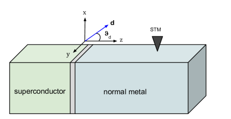
Figure 1: Schematic representation of the superconductor- insulator-normal metal junction. The vector ${\hat{z}}$ is along the c-axis of crystal, and $\vartheta_{\mathbf{d}}$ denotes the angle between spin vector $\mathbf{d}$ and $\hat{z}$. The dependence of the voltage inside the normal metal on the distance from the boundary may be measured by a scanning tunneling microscope (STM).

In this article we consider a p-wave superconductor-insulator-normal metal junction in the geometry in which the insulating boundary ($xy$-plane) is perpendicular to the c-axis of the layered chiral p-wave superconductor, as shown in Fig. (1). Although for simplicity we take the order parameter in the superconductor in the formAndersonMorel ; mineev

$$\hat{\Delta}({\bf n})=\Delta({\bf n})(\mathbf{d}\cdot\bm{\sigma})i\sigma_{2},\quad\Delta({\bf n})=\Delta_{0}e^{i\varphi_{\mathbf{n}}},$$ (1)

our results also apply to more complicated forms of the order parameter, such as for example that in Ref. kivelson, . Here $\mathbf{n}$ is a unit vector in the xy-plane, which points along $\mathbf{p}$, and $\varphi_{\mathbf{n}}$ is the azimuthal angle characterizing its direction $\mathbf{n}=(\cos\varphi_{\mathbf{n}},\sin\varphi_{\mathbf{n}})$.

At temperatures well below the gap, tunneling of single electrons from the metal to the superconductor is forbidden. Thus, similar to the s-wave case, the resistance of the junction is determined by the tunneling of the electron pairs. Coherent pair tunneling gives rise to coherence between electrons and holes inside the normal metal. Electron-hole coherence in the metal is characterized by the anomalous Green function. The crucial difference between the s-wave and the p-wave cases is the following. In the p-wave case in the absence of spin-orbit interaction only the p-wave component is induced inside the normal metal. The latter is exponentially suppressed at distances larger than $l$ away from the superconductor-normal metal boundary. As a result, in the diffusive regime the conductance of the junction is significantly suppressed. In the presence of the spin-orbit interaction the p-wave order parameter in the superconductor is partially converted to the s-wave component inside the normal metal. At low temperatures, the s-wave component propagates into the metal to large distances from the boundary. Consequently, it is this component that determines the low temperature resistance of the system.

We show below that Rashba-type spin-orbit coupling at the boundary between the normal metal and the p-wave superconductor leads to strong dependence of the resistance on the direction of the vector ${\bf d}$, which characterizes the spin structure of the order parameter in Eq. (1). Since the spin orientation of the order parameter may be controlled by an external magnetic fieldknight our predictions may be tested in experiment. Qualitatively, this dependence may be understood as follows. In our geometry (with the $z$-axis parallel to the c-axis of the crystal) the $z$-component of the total (orbital plus spin) angular momentum, $J_{z}=L_{z}+s_{z}$, is conserved during tunneling even in the presence of spin-orbit interaction. Therefore the s-wave singlet proximity effect in the normal metal is produced only by the pairs with $J_{z}=0$ in the p-wave superconductor. Since in our geometry the $z$-component of the orbital angular momentum in a $p_{x}+ip_{y}$ superconductor is $L_{z}=+1$ we conclude that only the part of the condensate with $s_{z}=-1$ induces the s-wave proximity effect in the normal metal. This condensate fraction corresponds to the the components of the vector $\mathbf{d}$ lying in the xy-plane.

II Kinetic scheme for description of electron transport in p-wave superconductor-normal metal junctions.

The conventional description of the electronic transport in superconductors based on the Boltzmann kinetic equation is valid when all spatial scales in the problem, including the mean free path $l$, are larger than the characteristic size of electron wave packets. At low temperatures, $L_{T}\gg l$, this condition is violated and this approach cannot be used for the description of the effects mentioned above.

The set of equations describing the electronic transport in s-wave superconductors in this situation has been derived in Ref. LarkinOvchinnikov, . Below we review a modification of this approach for the case where the superconducting part of the junction is a p-wave superconductor. The central object of this approach is the matrix Green function in the Keldysh space

$$\check{G}({\bf x}_{1};{\bf x}_{2})=\left(\begin{array}[]{cc}\hat{G}^{R}&\hat{G}^{K}\\ 0&\hat{G}^{A}\end{array}\right).$$ (2)

The retarded, advanced and Keldysh Green functions in this equation can be written in the following form

$$\hat{G}_{\ell\ell^{\prime}}^{R}(\mathbf{x}_{1};\mathbf{x}_{2}) = -i\theta(t_{1}-t_{2})\langle\{\psi_{\ell}(\mathbf{x}_{1}),\psi^{\dagger}_{\ell^{\prime}}(\mathbf{x}_{2})\}\rangle,$$ (3)

$$\hat{G}_{\ell\ell^{\prime}}^{A}(\mathbf{x}_{1};\mathbf{x}_{2}) =\! i\theta(t_{2}-t_{1})\langle\{\psi_{\ell}(\mathbf{x}_{1}),\psi^{\dagger}_{\ell^{\prime}}(\mathbf{x}_{2})\}\rangle,$$ (4)

$$\hat{G}^{K}_{\ell\ell^{\prime}}(\mathbf{x}_{1};\mathbf{x}_{2}) = -i\langle[\psi_{\ell}(\mathbf{x}_{1}),\psi^{\dagger}_{\ell^{\prime}}(\mathbf{x}_{2})]\rangle.$$ (5)

Here $\mathbf{x}=(\mathbf{r},t)$ denotes the space-time coordinate, and the indices $\ell,\ell^{\prime}=1...4$ label the four components of the fermion operator in the Nambu/spin space; $\psi_{1}=\psi_{\uparrow}$, $\psi_{2}=\psi_{\downarrow}$, $\psi_{3}=\psi_{\uparrow}^{\dagger}$, $\psi_{4}=\psi_{\downarrow}^{\dagger}$. Finally, the anticommutator and the commutator of operators $A$ and $B$ are denoted by $\{A,B\}$ and $[A,B]$ respectively.

Introducing the new variables, $\mathbf{x}=(\mathbf{r},t)=(\mathbf{x}_{1}+\mathbf{x}_{2})/2$, and $\mathbf{x}^{\prime}=(\mathbf{r}^{\prime},t^{\prime})=\mathbf{x}_{1}-\mathbf{x}_{2}$, we can define the quasiclassical Green function by Fourier transforming $\check{G}({\bf x}_{1};{\bf x}_{2})$ with respect to $\mathbf{x}^{\prime}$ and integrating over $\xi_{\mathbf{p}}=\varepsilon_{\mathbf{p}}-E_{F}$ as

$$\check{g}(\mathbf{x},\mathbf{n},\epsilon)=\frac{i}{\pi}\int d\xi_{\mathbf{p}}\int d^{4}x^{\prime}e^{i\epsilon t^{\prime}-i\mathbf{p}\mathbf{r}^{\prime}}\tau_{3}\check{G}(\mathbf{x}_{1};\mathbf{x}_{2}).$$ (6)

Here $E_{F}$ is the Fermi energy, $\varepsilon_{\mathbf{p}}$ is the electron energy spectrum, and $\mathbf{n}$ is a unit vector labeling a location on the Fermi surface (for example, for a spherical Fermi surface it can be chosen as $\mathbf{n}=\mathbf{p}/|\mathbf{p}|$), and $\tau_{3}$ is the third Pauli matrix. In this paper, we will denote the Pauli matrices in the Nambu space by $\tau_{i}$, and the Pauli matrices in spin space by $\sigma_{i}$. The Keldysh space structure of the Green functions will be indicated explicitly when necessary.

The quasiclassical Green’s function (6) satisfies the normalization condition

$$\check{g}\check{g}=1,$$ (7)

which can be spelled out in terms of components in the Keldysh space as,

$$\hat{g}^{(R,A)}\hat{g}^{(R,A)}=1,$$ (8)

$$\hat{g}^{R}\hat{g}^{K}+\hat{g}^{K}\hat{g}^{A}=0.$$ (9)

The normalization condition Eq. (9) is satisfied for any Keldysh function of the form

$$\hat{g}^{K}=\hat{g}^{R}\hat{h}-\hat{h}\hat{g}^{A}.$$ (10)

The matrix $\hat{h}$ may be parameterized asLarkinOvchinnikov

$$\hat{h}=f_{0}\hat{\tau}_{0}+f_{1}\hat{\tau}_{3}.$$ (11)

Here $f_{0}$ and $f_{1}$ are respectively the odd and even in $\epsilon$ parts of the distribution function (see Ref. shelankov, for an alternative treatment).

In this paper we only consider stationary situations. In this case the Green functions depend on the energy $\epsilon$ but not on the time $t$. If $k_{F}l\gg 1$ the Gorkov equation for the Green function in Eq. (2) can be reduced to the quasi-classical Eilenberger equations for the Green functions defined in Eq. (6) LarkinOvchinnikov

$$i\mathbf{v}_{F}\cdot\bm{\nabla}\check{g}+\left[\epsilon\check{\tau}_{3}-\check{\Delta}(\mathbf{n})-\check{\Sigma},\check{g}\right]=0.$$ (12)

Here $\check{\Sigma}$ is the self energy associated with impurity scattering. In the Born approximation $\check{\Sigma}=-i\langle\check{g}\rangle/2\tau_{e}$, where $\langle\ldots\rangle$ denotes average over the solid angle in momentum space and $\tau_{e}$ is the elastic mean free time. The only difference of Eq. (12) from the conventional s-wave superconductor case is in the form Eq. (1) for the order parameter.

We neglect the electron-electron interactions in the normal metal. As a result, in our approximation the order parameter vanishes inside the normal metal. This yields the following equations for the retarded, advanced and Keldysh Green functions:

$$i\mathbf{v}_{F}\cdot\bm{\nabla}\hat{g}^{R,A}+\epsilon[\hat{\tau}_{3},\hat{g}^{R,A}] = [\hat{\Sigma}^{R,A},\hat{g}^{R,A}],$$ (13)

$$i\mathbf{v}_{F}\cdot\bm{\nabla}\hat{g}^{K}+\epsilon[\tau_{3},\hat{g}^{K}] = \hat{\Sigma}^{R}\hat{g}^{K}+\hat{\Sigma}^{K}\hat{g}^{A}$$ (14)

$$-\hat{g}^{R}\hat{\Sigma}^{K}-\hat{g}^{K}\hat{\Sigma}^{A}.$$

Multiplying Eq. (14) with $\tau_{3}$ and $\tau_{0}$ and taking the trace, and using the fact that $\mathrm{Tr}(\hat{g}^{R}-\hat{g}^{A})=0$, one obtains the following equations for $f_{1}$ and $f_{0}$

$$\mathrm{Tr}\left[\hat{\beta}\right]\mathbf{v}_{F}\cdot\bm{\nabla}f_{1} = -\frac{1}{2\tau_{e}}f_{0}\mathrm{Tr}\left(\langle\hat{\alpha}\rangle\hat{\alpha}-[\langle\hat{g}^{R}\rangle,\hat{g}^{R}]+[\langle\hat{g}^{A}\rangle,\hat{g}^{A}]\right)+\frac{1}{2\tau_{e}}\mathrm{Tr}\left[\langle\hat{\alpha}f_{0}\rangle\hat{\alpha}\right]$$ (15)

$$- \frac{1}{2\tau_{e}}f_{1}\mathrm{Tr}\left(\langle\hat{\alpha}\rangle\hat{\beta}-[\langle\hat{g}^{R}\rangle,\hat{g}^{R}]\hat{\tau}_{3}+\hat{\tau}_{3}[\langle\hat{g}^{A}\rangle,\hat{g}^{A}]\right)+\frac{1}{2\tau_{e}}\mathrm{Tr}\left[\langle\hat{\beta}f_{1}\rangle\hat{\alpha}\right],$$

$$\mathrm{Tr}\left[\hat{\beta}\right]\mathbf{v}_{F}\cdot\bm{\nabla}f_{0} = -\frac{1}{2\tau_{e}}f_{0}\mathrm{Tr}\left(\langle\hat{\tau}_{3}\hat{\beta}\hat{\tau}_{3}\rangle\hat{\alpha}-[\langle\hat{g}^{R}\rangle,\hat{g}^{R}]\hat{\tau}_{3}+\hat{\tau}_{3}[\langle\hat{g}^{A}\rangle,\hat{g}^{A}]\right)+\frac{1}{2\tau_{e}}\mathrm{Tr}\left[\langle\hat{\alpha}f_{0}\rangle\hat{\tau}_{3}\hat{\beta}\hat{\tau}_{3}\right]$$ (16)

$$- \frac{1}{2\tau_{e}}f_{1}\mathrm{Tr}\left(\langle\hat{g}^{R}\rangle\hat{\beta}\hat{\tau}_{3}-\hat{\tau}_{3}\hat{\beta}\langle\hat{g}^{A}\rangle-[\langle\hat{g}^{R}\rangle,\hat{g}^{R}]+[\langle\hat{g}^{A}\rangle,\hat{g}^{A}]\right)+\frac{1}{2\tau_{e}}\mathrm{Tr}\left[\langle\hat{\beta}f_{1}\rangle\hat{\tau}_{3}\hat{\beta}\hat{\tau}_{3}\right].$$

Here we defined $\hat{\alpha}=\hat{g}^{R}-\hat{g}^{A}$ and $\hat{\beta}=\hat{g}^{R}\hat{\tau}_{3}-\hat{\tau}_{3}\hat{g}^{A}$.

The gauge-invariant potential and the electric current can be expressed in terms of quasiclassical Keldysh green functions as,

$$\Phi(\mathbf{r}) = \frac{1}{4e}\int d\epsilon\int d^{2}\mathbf{n}\mathrm{Tr}\{\hat{g}^{K}(\mathbf{r},\mathbf{n},\epsilon)\}$$ (17)

$$J(\mathbf{r}) = -\frac{e\nu_{0}}{4}\int d\epsilon\int d^{2}\mathbf{n}\mathbf{v}_{F}\mathrm{Tr}\{\hat{\tau}_{3}\hat{g}^{K}(\mathbf{r},\mathbf{n},\epsilon)\}.$$ (18)

Here the integral over $\mathbf{n}$ denotes averaging over the Fermi surface, $d^{2}\mathbf{n}=d\Omega_{\mathbf{n}}/4\pi$.

We discuss the boundary conditions for the quasiclassical transport equations (12) - (16) in Sec. II.1.

II.1 Boundary conditions for p-wave superconductor-normal metal interface

The p-wave superconductivity is destroyed by elastic scattering processes when $l<\xi_{0}$, where $\xi_{0}$ is the zero temperature coherence length in a clean superconductor. Therefore we consider the case where the p-wave superconductor is relatively clean and $l\gg\xi$. For the same reason the p-wave proximity effect is exponentially suppressed in the metal at distances larger than $l$ from the boundary. On the other hand, in a spatially inhomogeneous system in the presence of spin-orbit interaction the p- and s- wave components of the anomalous Green functions are mixed. At low temperatures, the s-wave component induced by spin-orbit coupling extends into the metal to distances much larger than $l$, and determines the low temperature transport properties of the junction. Therefore spin-orbit coupling plays a crucial role in low temperature electron transport in normal metal–p-wave superconductor junctions.

Though our results have a general character, in this article we assume that a Rashba type spin orbit coupling is present only at the boundary. The corresponding potential energy at the boundary may be modeled by the form $V=(u_{0}\sigma_{0}+u_{1}\hat{z}\times\mathbf{p}_{\parallel}\cdot\bm{\sigma})\delta(z)$, where $\mathbf{p}_{\parallel}$ is the component of the electron momentum parallel to the boundary, and $\hat{z}$ is the unit vector normal to the boundary. We assume that $u_{1}\ll u_{0}$, and consider a disorder free boundary, so that $\mathbf{p}_{\parallel}$ is conserved.

The boundary conditions for quasiclassical Green functions in superconductors were obtained in Refs. zaitsev, ; millis, ; kuprianov, . In the case of a spin active boundary millis they may be expressed in terms of the $\mathbf{p}_{\parallel}$-dependent scattering matrix of the insulating barrier. The latter relates the spinor amplitudes of the outgoing ($\psi_{o}$) and incident ($\psi_{i}$) electron waves,

$$\left(\begin{array}[]{c}\psi_{o}^{S}\\ \psi_{o}^{N}\\ \end{array}\right)=\left(\begin{array}[]{cc}S_{11}&S_{12}\\ S_{21}&S_{22}\\ \end{array}\right)\left(\begin{array}[]{c}\psi_{i}^{S}\\ \psi_{i}^{N}\\ \end{array}\right).$$ (19)

Here the superscripts $N$ and $S$ denote respectively the normal metal and the superconductor side of the barrier. The presence of spin-orbit interaction at the boundary results in a spin-dependent transmission amplitude $S_{12}$, which may be written in the form

$$S_{12} = t_{0}+t_{s}\gamma(\varphi_{\mathbf{n}}),$$ (20)

$$\gamma(\varphi_{\mathbf{n}}) = \cos\varphi_{\mathbf{n}}\sigma_{y}-\sin\varphi_{\mathbf{n}}\sigma_{x}.$$ (21)

Here we introduced the azimuthal angle $\varphi_{\mathbf{n}}$ as $\mathbf{p}_{\parallel}=|\mathbf{p}_{\parallel}|(\hat{x}\cos\varphi_{\mathbf{n}}+\hat{y}\sin\varphi_{\mathbf{n}})$. The spin-dependent and spin-independent transmission amplitudes $t_{s}$ and $t_{0}$, are scalar functions of $|\mathbf{p}_{\parallel}|$. To lowest order in the transmission amplitude, the boundary condition for the quasiclassical Green functions may be written as millis

$$\check{g}(\mathbf{r}^{N},\mathbf{n}^{N}_{{o}}) = -\frac{1}{2}\left[\check{S}_{21}\left(\check{g}(\mathbf{r}^{S},\mathbf{n}^{S}_{{i}})-1\right)\check{S}^{\dagger}_{21},\check{g}(\mathbf{r}^{N},\mathbf{n}^{N}_{{o}})\right]$$ (22)

$$+\check{S}_{22}\check{g}(\mathbf{r}^{N},\mathbf{n}^{N}_{{i}})\check{S}^{-1}_{22},$$

$$\check{g}(\mathbf{r}^{S},\mathbf{n}^{S}_{{i}}) = -\frac{1}{2}\left[\check{g}(\mathbf{r}^{S},\mathbf{n}^{S}_{{i}}),\check{S}_{21}^{\dagger}\left(\check{g}(\mathbf{r}^{N},\mathbf{n}^{N}_{{o}})-1\right)\check{S}_{21}\right]$$ (23)

$$+\check{S}^{-1}_{11}\check{g}(\mathbf{r}^{S},\mathbf{n}^{S}_{{o}})\check{S}_{11}.$$

Here $\mathbf{n}_{i,o}^{S}$ and $\mathbf{n}_{i,o}^{N}$ are the unit vectors indicating positions on the Fermi surface in the superconductor ($S$) and the normal metal ($N$) for the incident ($i$) and outgoing ($o$) waves. By momentum conservation they correspond to the same $\mathbf{p}_{\parallel}$ and thus are characterized by the same azimuthal angle $\varphi_{\mathbf{n}}$. For simplicity we assume that Fermi surface in the superconductor to be a corrugated cylinder with the symmetry axis along $\hat{z}$, and that in the normal metal to be a sphere. The Fermi surface points corresponding to the incident and reflected waves are illustrated in Fig. 2. The coordinates $\mathbf{r}^{N}$ and $\mathbf{r}^{S}$ correspond respectively to the normal metal - and the superconductor- sides of the insulating boundary. For brevity the obvious $\epsilon$ dependence of Green functions has been dropped. Finally the matrices $\check{S}_{\alpha\beta}$ are defined following Ref. millis, as

$$\check{S}_{\alpha\beta}=S_{\alpha\beta}(\mathbf{p}_{\parallel})\frac{1+\tau_{3}}{2}+S_{\beta\alpha}(-\mathbf{p}_{\parallel})^{T}\frac{1-\tau_{3}}{2},$$ (24)

where $S_{\alpha\beta}$ is defined in Eq. (20) and the superscript ${T}$ denotes the matrix transposition in the spin space. At weak tunneling we may approximate $\check{S}_{11}\approx\check{S}_{22}\approx 1$, and

$$\check{S}_{12}=t_{0}\check{1}+t_{s}\check{\gamma}.$$ (25)

Here we introduced

$$\check{\gamma}=\left(\begin{array}[]{cc}\hat{\gamma}&0\\ 0&\hat{\gamma}\\ \end{array}\right),\quad\hat{\gamma}=\left(\begin{array}[]{cc}\gamma(\varphi_{\mathbf{n}})&0\\ 0&-\gamma(\varphi_{\mathbf{n}})^{T}\\ \end{array}\right).$$ (30)

with $\gamma(\varphi_{\mathbf{n}})$ defined in Eq. (21).

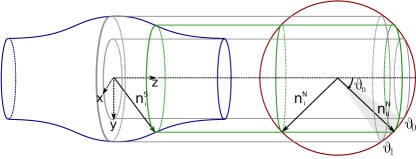
Figure 2: Fermi surface topologies of the superconductor (corrugated cylinder at left) and the normal metal (sphere at right). The vectors $\mathbf{n}_{i}$ and $\mathbf{n}_{o}$ correspond to respectively incident and outgoing waves. The superscripts $N$ and $S$ denote the superconductor and the normal metal sides of the insulating barrier. The vectors $\mathbf{n}^{N}$ and $\mathbf{n}^{S}$ correspond to the same parallel momentum, as shown by the green lines. The momentum domain where tunneling is possible is bounded by the angles $\vartheta_{0}$ and $\vartheta_{1}$. These angles define the integration limits in Eqs. (56) and (61).

For the purpose of studying electron transport at low temperatures, $T\ll\Delta$, we only need the Green functions with energies $\epsilon$ well below the gap $\Delta$. The Green functions inside the superconductor are practically unaffected by tunneling. Therefore, the boundary condition for the normal metal Green function is given by Eq. (22), where the superconductor Green functions are replaced by their value in the bulk. Since latter do not depend on $p_{z}$ we have $\check{g}(\mathbf{r}^{S},\mathbf{n}_{i}^{S})=\check{g}(\mathbf{r}^{S},\mathbf{n}_{o}^{S})\equiv\check{g}(\mathbf{r}^{S},\mathbf{n}^{S})$. It is useful to define symmetric and antisymmetric Green functions as (zaitsev, ; kuprianov, )

$$\check{g}_{s,a}(\mathbf{r},\mathbf{n})=\frac{1}{2}[\check{g}(\mathbf{r},\mathbf{n}_{i})\pm\check{g}(\mathbf{r},\mathbf{n}_{o})]$$ (31)

With this notation Eq. (22) may be written as follows:

$$\check{g}_{a}(\mathbf{r}^{N},\mathbf{n}^{N}) = -\frac{t_{0}^{2}}{4}\left[\check{g}(\mathbf{r}^{S},\mathbf{n}^{S}),\check{g}_{s}(\mathbf{r}^{N},\mathbf{n}^{N})\right]$$ (32)

$$-\frac{t_{0}t_{s}}{4}\left[\left\{\check{\gamma},\check{g}(\mathbf{r}^{S},\mathbf{n}^{S})\right\},\check{g}_{s}(\mathbf{r}^{N},\mathbf{n}^{N})\right]$$

$$+\frac{t_{0}t_{s}}{2}\left[\check{\gamma},\check{g}_{s}(\mathbf{r}^{N},\mathbf{n}^{N})\right].$$

Here we for simplicity assume that due to weakness of spin-orbit coupling the electron tunneling amplitude with spin flip is smaller than that without, $t_{s}\ll t_{0}\ll 1$. The first term in Eq. (32) arises from the spin-conserving tunneling and coincides with that in Ref. zaitsev, at small transparency. This term dominates electron transport properties of the junction in the high temperature regime. The second term comes from the spin orbit coupling. Although it is smaller than the first one, it generates the s-wave component proximity effect in the normal metal and thus determines the electron transport at low temperatures. Finally, the last term is odd in the parallel momentum. Therefore it vanishes upon averaging over the Fermi surface and does not contribute to electron transport in the diffusive regime.

II.2 Kinetic scheme in the diffusive regime

In the low temperature regime, $T\ll v_{F}/l$, the proximity effect extends to distances of order $L_{T}=\sqrt{D/T}\gg l$ into the normal metal (here $D$ is the electron diffusion constant). At such length scales the transport properties of the junction may be described in terms of the Usadel Green functions $\check{G}(\mathbf{r})$. The latter correspond to coincident coordinates of the electron operators in Eq. (2), $\mathbf{r}=\mathbf{r}^{\prime}$, and may be expressed in terms of the Eilenberger Green functions (6) by averaging them over the Fermi surface

$$\check{G}(\mathbf{r})=\int d^{2}\mathbf{n}\,\check{g}(\mathbf{r},\mathbf{n}),\quad d^{2}\mathbf{n}=\frac{1}{4\pi}\,d\cos\vartheta_{\mathbf{n}}d\varphi_{\mathbf{n}}.$$ (33)

where the polar and azimuthal angles $\vartheta_{\mathbf{n}}$ and $\varphi_{\mathbf{n}}$ characterize the unit vector $\mathbf{n}=(n_{x},n_{y},n_{z})=(\sin\vartheta_{\mathbf{n}}\cos\varphi_{\mathbf{n}},\sin\vartheta_{\mathbf{n}}\sin\varphi_{\mathbf{n}},\cos\vartheta_{\mathbf{n}})$.

We neglect the spin-orbit interaction in the normal metal and assume that the electrons in the normal lead are not spin polarized. The triplet component of the anomalous Green function is exponentially suppressed at distances larger than $l$ from the boundary with the superconductor. The singlet component, on the other hand, survives even at distances much larger than $l$. Therefore it dominates the electron transport in the junction at low temperatures. Below we focus on the singlet component of the Usadel Green function, $\hat{G}(\mathbf{r})$, which is a $4\times 4$ matrix in the Keldysh and Nambu space. Its various components $\alpha=R,A,K$ in the Keldysh space have the following form

$$\hat{G}^{\alpha}(\mathbf{r})=\left(\begin{array}[]{ccc}G^{\alpha}&-iF^{\alpha}\\ i\tilde{F}^{\alpha}&-\tilde{G}^{\alpha}\end{array}\right).$$ (34)

The corresponding spin structure of the full $8\times 8$ Green function in Eq. (33) is given by

$$\check{G}^{\alpha}(\mathbf{r})=\left(\begin{array}[]{ccc}G^{\alpha}\sigma_{0}&-iF^{\alpha}i\sigma_{2}\\ i\tilde{F}^{\alpha}i\sigma_{2}&-\tilde{G}^{\alpha}\sigma_{0}\end{array}\right).$$ (35)

At length scales greater than $l$ the singlet component of the Usadel Green function satisfies the differential equation

$$D\bm{\nabla}\cdot\left[\hat{G}(\mathbf{r})\bm{\nabla}\hat{G}(\mathbf{r})\right]+i\epsilon\left[\hat{\tau}_{3},\hat{G}(\mathbf{r})\right]=0.$$ (36)

Expanding in the Keldysh space, this equation gives

$$D\bm{\nabla}\cdot\left(\hat{G}^{(R,A)}\bm{\nabla}\hat{G}^{(R,A)}\right)+i\epsilon[\hat{\tau}_{3},\hat{G}^{(R,A)}]=0,$$ (37)

$$D\bm{\nabla}\cdot\left(\hat{G}^{R}\bm{\nabla}\hat{G}^{K}+\hat{G}^{K}\bm{\nabla}\hat{G}^{A}\right)+i\epsilon[\hat{\tau}_{3},\hat{G}^{K}]=0.$$ (38)

The first equation (37) is the Usadel equation, which describes the equilibrium properties of the system. The second equation (38) for Keldysh component describes the non-equilibrium properties. The Usadel Green function satisfies the normalization conditions (8) and (9). The condition (9) is satisfied by any matrix of the form (10). In the normal metal the matrix $\hat{h}$ may be expressed in terms of the symmetric and antisymmetric distribution functions $f_{0}$ and $f_{1}$ using Eq. (11). LarkinOvchinnikov

In a normal metal in contact with a single superconducting lead, Eq. (38) can be used to obtain following equations for distribution functions by using Eqs. (10) and (11):

$$\bm{\nabla}\cdot\left(\mathrm{Tr}\left[1-\hat{G}^{R}(\mathbf{r})\hat{G}^{A}(\mathbf{r})\right]\bm{\nabla}f_{0}(\mathbf{r},\epsilon)\right) = 0,$$ (39)

$$\bm{\nabla}\cdot\left(\mathrm{Tr}\left[1-\tau_{3}\hat{G}^{R}(\mathbf{r})\tau_{3}\hat{G}^{A}(\mathbf{r})\right]\bm{\nabla}f_{1}(\mathbf{r},\epsilon)\right) = 0.$$ (40)

The expressions for the density of states, electrochemical potential and current density in terms of the Usadel Green functions are

$$\nu(\mathbf{r},\epsilon) = \nu_{0}\mathrm{Re}\left\{G^{R}(\mathbf{r},\epsilon)\right\},$$ (41)

$$\Phi(\mathbf{r}) = \frac{1}{e\nu_{0}}\int d\epsilon\nu(\mathbf{r},\epsilon)f_{1}(\mathbf{r},\epsilon),$$ (42)

$$J(\mathbf{r}) = e\nu_{0}D\int d\epsilon\Pi(\mathbf{r},\epsilon)\bm{\nabla}f_{1}(\mathbf{r},\epsilon).$$ (43)

Here $\Pi(\mathbf{r},\epsilon)=1+|G^{R}(\mathbf{r},\epsilon)|^{2}+|F^{R}(\mathbf{r},\epsilon)|^{2}$, $\nu_{0}=mp_{F}/\pi^{2}$ is the density of states of the normal metal in the absence of the proximity effect.

Using Eq. (8) one can write the retarded Usadel Green function in terms of the complex angles $\theta(\mathbf{r})$ and $\chi(\mathbf{r})$ as

$$\hat{G}^{R}(\mathbf{r})=\left(\begin{array}[]{cc}\cos\theta(\mathbf{r})&-i\sin\theta(\mathbf{r})e^{i\chi(\mathbf{r})}\\ i\sin\theta(\mathbf{r})e^{-i\chi(\mathbf{r})}&-\cos\theta(\mathbf{r})\\ \end{array}\right).$$ (44)

The corresponding parametrization for advanced Green function can be obtained by using $\hat{G}^{A}(\mathbf{r})=-\tau_{3}\left[\hat{G}^{R}(\mathbf{r})\right]^{\dagger}\tau_{3}$.

For the system of interest, where the normal metal is connected to a single superconductor the phase $\chi(\mathbf{r})$ is independent of coordinates and is set by the phase of the order parameter in the superconductor. In this case ($\bm{\nabla}\chi(\mathbf{r})=0$) the Usadel equation in (37) reduces to the following second order differential equation for the complex function $\theta(\mathbf{r})$:

$$\frac{D}{2}\bm{\nabla}^{2}\theta(\mathbf{r})+i\epsilon\sin\theta(\mathbf{r})=0,$$ (45)

which is the well known sine-Gordon equation.

The equations for the distribution functions in (39) and (40) take the following forms in this parametrization:

$$D\bm{\nabla}\cdot\left(\cos^{2}\theta_{R}(\mathbf{r})\bm{\nabla}f_{0}(\mathbf{r})\right) = 0,$$ (46)

$$D\bm{\nabla}\cdot\left(\cosh^{2}\theta_{I}(\mathbf{r})\bm{\nabla}f_{1}(\mathbf{r})\right) = 0.$$ (47)

Here we introduced the real and imaginary parts of $\theta(\mathbf{r})=\theta_{R}(\mathbf{r})+i\theta_{I}(\mathbf{r})$.

Finally, using Eqs. (42), (43), and (44) we get the following expressions for the electric current and potential

$$J_{n}(\mathbf{r}) = eD\nu_{0}\int d\epsilon\cosh^{2}\theta_{I}(\mathbf{r})\bm{\nabla}f_{1}(\mathbf{r})$$ (48)

$$\Phi(\mathbf{r}) = \frac{1}{e}\int d\epsilon\cos\theta_{R}(\mathbf{r})\cosh\theta_{I}(\mathbf{r})f_{1}(\mathbf{r}).$$ (49)

Below we will be interested only in linear in the external electric field effects, in which case $f_{0}=\tanh(\epsilon/2T)$, has its equilibrium form.

The equations (37-38) or (45-47) must be supplemented with the boundary conditions. In Sec. II.2.1 we obtain such conditions for a boundary between the normal metal and the p-wave superconductor in the geometry of our device.

II.2.1 Diffusive Boundary Conditions in the Vertical Geometry

The boundary conditions for the Usadel Green function $\hat{G}(\mathbf{r})$ may be found by solving the Eilenberger equations (12) with boundary conditions (32) at distances of the order of the mean free path $l$ from the boundary. This can be done using the method of Ref. kuprianov, . A key observation is that the Eilenberger equations (in which one may set $\epsilon\to 0$ for distances less than the mean free path from the boundary) conserve the matrix current normal to the boundary,

$$\check{j}(\mathbf{r})=\int d^{2}\mathbf{n}\check{g}({\bf r},\mathbf{n})\mathbf{v}_{F}\cdot\hat{z}=v_{F}\int^{\prime}d^{2}\mathbf{n}\check{g}_{a}({\bf r},\mathbf{n})\mathbf{n}\cdot\hat{z}.$$ (50)

The prime in the second expression indicates the fact that the integral must be taken over half the Fermi surface, $\mathbf{n}\cdot\hat{z}\geq 0$.

At weak tunneling the singlet component $\hat{j}$ of the matrix current at the boundary may be expressed in terms of the Usadel Green function $\hat{G}(\mathbf{r})$ askuprianov

$$\hat{j}(\mathbf{r}^{N})=D\hat{G}(\mathbf{r})\hat{z}\cdot\bm{\nabla}\hat{G}(\mathbf{r})|_{\mathbf{r}=\mathbf{r}^{N}}.$$ (51)

On the other hand, the matrix current may be evaluated by multiplying Eq. (32) with $v_{F}\mathbf{n}^{N}\cdot\hat{z}$ and integrating the result over half the Fermi surface, $\mathbf{n}^{N}\cdot\hat{z}\geq 0$. In doing so it is important to keep in mind that at weak tunneling the symmetric part of Green function in the normal metal is independent of $\mathbf{n}^{N}$, $\check{g}_{s}(\mathbf{r}^{N},\mathbf{n}^{N})=\check{G}(\mathbf{r}^{N})$, and that the superconductor Green function $\check{g}_{s}(\mathbf{r}^{S},\mathbf{n}^{S})$ may be replaced by its bulk value at $\epsilon=0$. The latter is given by

$$\check{g}(\mathbf{n})=-\left[\begin{array}[]{cc}0&e^{i(\varphi_{\mathbf{n}}+\chi_{0})}\mathbf{d}\cdot\bm{\sigma}i\sigma_{2}\\ e^{-i(\varphi_{\mathbf{n}}+\chi_{0})}i\sigma_{2}\mathbf{d}^{*}\cdot\bm{\sigma}&0\end{array}\right].$$ (54)

Here we used Eq. (1). We consider unitary states, $\mathbf{d}\times\mathbf{d}^{*}=0$, and parameterize the vector $\mathbf{d}$ by an overall phase $\chi_{0}$ and the spherical angles $\vartheta_{\mathbf{d}}$, and $\varphi_{\mathbf{d}}$ as,

$$\mathbf{d}^{T}=e^{i\chi_{0}}(\sin\vartheta_{\mathbf{d}}\cos\varphi_{\mathbf{d}},\sin\vartheta_{\mathbf{d}}\sin\varphi_{\mathbf{d}},\cos\vartheta_{\mathbf{d}}).$$ (55)

It is easy to see that only the second term in the right hand side of Eq. (32) contributes to the matrix current. The contributions of the other two terms vanish upon the integration over $\mathbf{n}$ because both $\check{\gamma}$ and the superconductor Green function $\check{g}(\mathbf{r}^{S},\mathbf{n}^{S})$ depend on the azimuthal angle $\varphi_{\mathbf{n}}$ as $e^{\pm i\varphi_{\mathbf{n}}}$, see Eqs. (21), (30) and (54). We thus obtain

$$\check{j}(\mathbf{r})=-\frac{v_{F}}{4}\int_{\vartheta_{0}}^{\vartheta_{1}}\frac{d\cos\vartheta_{\mathbf{n}}}{2}t_{s}t_{0}\hat{z}\cdot\mathbf{n}\left[\check{\bar{G}}(\mathbf{r}^{S}),\check{G}(\mathbf{r}^{N}).\right]$$ (56)

Here $v_{F}$ is Fermi velocity in the normal metal, and the integration limits $\vartheta_{0}$ and $\vartheta_{1}$ define the domain where tunneling is possible. This domain corresponds to the projection of the corrugated cylindrical Fermi surface in the superconductor to the Fermi surface in the metal, see Fig. 2. Finally, $\check{\bar{G}}(\mathbf{r}^{S})$ is given by

$$\check{\bar{G}}(\mathbf{r}^{S}) \equiv \int\frac{d\varphi_{\mathbf{p}}^{S}}{2\pi}\left\{\check{g}(\mathbf{r}^{S},\mathbf{n}^{S}_{i}),\check{\gamma}\right\}$$ (59)

$$= \left[\begin{array}[]{cc}0&e^{i(\varphi_{\mathbf{d}}+\chi_{0})}i\sigma_{2}\\ e^{-i(\varphi_{\mathbf{d}}+\chi_{0})}i\sigma_{2}&0\end{array}\right].$$

Comparing Eqs. (51) and (56) we obtain the following boundary condition for the Usadel Green function,

$$D\check{G}(\mathbf{r})\partial_{z}\check{G}(\mathbf{r})|_{\mathbf{r}=\mathbf{r}^{N}}=t\left[\check{G}(\mathbf{r}^{N}),\check{\bar{G}}(\mathbf{r}^{S})\right],$$ (60)

where

$$t=\frac{1}{4}|\sin\vartheta_{\mathbf{d}}|\int_{\vartheta_{0}}^{\vartheta_{1}}\frac{d\cos\vartheta_{\mathbf{n}}}{2}(t_{s}t_{0}v_{F}\cos\vartheta_{\mathbf{n}}).$$ (61)

Note that the boundary condition in Eq. (60) has the same structure as that for a boundary between an normal metal and an s-wave superconductor. The reason is that only the s-wave component of the anomalous Green function survives in the normal metal at distances larger than $l$ from the boundary. The difference however is that in our case the effective barrier transparency $t$ in Eq. (61) depends on the spin-flip tunneling amplitude $t_{s}$, and on the vector $\mathbf{d}$ characterizing the spin orientation of the triplet order parameter. The phase of the effective s-wave anomalous Green function (59), $\chi_{0}+\varphi_{\mathbf{d}}$, also depends on the orientation of the spin vector $\mathbf{d}$ in the xy-plane.

The aforementioned analogy enables one to treat the proximity effect in normal metal- p-wave superconductor systems in the diffusive regime as proximity effect in an effective s-wave superconductor problem, in which the phase of the s-wave order parameter and the barrier transparency depend on the spin orientation of the p-wave condensate.

It is convenient to recast the boundary condition Eq. (60) in terms of the parametrization in Eq. (44). In our setup, see Fig. 1, the phase $\chi(\mathbf{r})$ of the anomalous Usadel Green function (44) is uniform in space and equal to the phase of the effective s-wave order parameter, $\chi(\mathbf{r})=\varphi_{\mathbf{n}}+\chi_{0}$. The boundary condition for the angle $\theta(\mathbf{r}^{N})$ becomes

$$D\partial_{z}\theta(\mathbf{r})\big{|}_{\mathbf{r}=\mathbf{r}^{N}}=2t\cos\left[\theta(\mathbf{r}^{N})\right].$$ (62)

The Keldysh component of the boundary condition in Eq. (60) gives the following boundary condition for the even part of the distribution function:

$$D\cosh^{2}\theta_{I}(\mathbf{r})\partial_{z}f_{1}(\mathbf{r})|_{\mathbf{r}=\mathbf{r}^{N}} = 2t\Gamma_{\epsilon}f_{1}(\mathbf{r}^{N}).$$ (63)

Here we assumed that $f_{1}(\mathbf{r}^{S})=0$ is zero inside superconductor and introduced the notation

$$\Gamma_{\epsilon}=\cosh\theta_{I}(\mathbf{r}^{N})\sin\theta_{R}(\mathbf{r}^{N}).$$ (64)

The set of equations (45) and (47) along with the boundary conditions (62) and (63) gives a description of electron transport in diffusive metal–p-wave superconductor systems. Below we apply these equations to our device geometry.

III Resistance of p-wave superconductor- normal metal junction

We consider the geometry in which the superconductor fills the $z<0$ half space and the normal metal occupies the $z>0$ half space, see Fig. 1. At weak tunneling the Green function in the superconductor is practically unaffected by the presence of the tunneling barrier. On the other hand, the low energy properties of the normal metal are significantly affected by the proximity effect. The singlet Usadel Green function (34) in the normal metal is described by the set of equations (44), (45), (47) with the boundary conditions (62) and (63).

The solution of Eq. (45) satisfying the condition $\lim_{z\to\infty}\theta(z)=0$, has the form

$$\theta(\epsilon,z)=4\arctan\left[\exp\left(\beta_{\epsilon}+(i-1)\frac{z}{L_{\epsilon}}\right)\right].$$ (65)

Here $\beta_{\epsilon}$ is an energy-dependent integration constant. Its value is determined from the boundary condition in Eq. (62), which gives

$$\cosh\beta_{\epsilon}-\frac{2}{\cosh\beta_{\epsilon}}=(1-i)\frac{L_{t}}{L_{\epsilon}}$$ (66)

where

$$L_{t}=\frac{D}{t},\quad L_{\epsilon}=\sqrt{\frac{D}{\epsilon}}.$$ (67)

The algebraic equation (66) has multiple solutions for the integration constant $\beta_{\epsilon}$. The physical solution must satisfy the condition $\lim_{\epsilon\to 0}\theta(\epsilon,z=0+)=\pi/2$, which gives

$$e^{\beta_{\epsilon}}=\frac{\alpha+\sqrt{\alpha^{2}+8}}{2}-\frac{1}{2}\sqrt{(\alpha+\sqrt{\alpha^{2}+8})^{2}-4},$$ (68)

where we introduced the notation $\alpha=(1-i)L_{t}/L_{\epsilon}$.

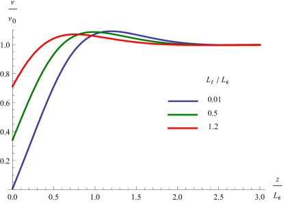
Figure 3: (color online) Density of states in the normal metal as a function of the distance from the superconductor-normal metal boundary for different temperatures: $L_{t}/L_{\epsilon}=0.01$ (blue), $L_{t}/L_{\epsilon}=0.5$ (green), and $L_{t}/L_{\epsilon}=1.2$ (red).

An important aspect of the solution Eq. (65) is that in the normal metal, at small values of $\epsilon$ and at small distances from the boundary, $\theta(z)\approx\pi/2$ which is the same as in the bulk of the superconductor. In particular, it means that at small energies the density of states in metal is strongly suppressed at distances smaller than $L_{\epsilon}$. The full spatial dependence of the density of states $\nu(\epsilon,z)$ may be obtained by substituting the solution (65), (68) of the Usadel equation into Eqs. (41), and (44). In Fig. 3 we have plotted the result as a function of $z/L_{\epsilon}$ for different values of $L_{t}/L_{\epsilon}$.

Note that the effective diffusion constant for the distribution function $f_{1}$ is determined by the imaginary part of $\theta$, see Eq. (47). From the solution (65) it follows that the imaginary part $\theta_{I}$ is close to zero both at $z\gg L_{\epsilon}$ and $z\ll L_{\epsilon}$ and has a maximum at $z\sim L_{\varepsilon}$ whose value depends on $L_{\epsilon}/L_{t}$. Therefore the effective diffusion coefficient in Eq. (47) approaches its normal metal value at $z\gg L_{\epsilon}$ and $z\ll L_{\epsilon}$. In the intermediate region $z\sim L_{\epsilon}$ the diffusion coefficient exceeds the Drude value.

The differential equation (47) for the non-equilibrium part of the distribution function has the first integral, which has the meaning of the conserved partial current density at a given energy $\epsilon$

$$J_{\epsilon}\equiv eD\nu_{0}\cosh^{2}\theta_{I}(z)\partial_{z}f_{1}(\epsilon,z).$$ (69)

The energy dependence of the partial current $J_{\epsilon}$ can be obtained by noticing that far away form the boundary the distribution function should have the form

$$f_{1}(\epsilon,z)=\frac{1}{\cosh^{2}\frac{\epsilon}{2T}}\frac{eJ_{0}}{2T\sigma_{D}}(z-z_{0}),$$ (70)

where $\sigma_{D}=e^{2}\nu_{0}D$ is the Drude conductivity of the normal metal, and we introduced the current density,

$$J_{0}=\int_{-\infty}^{\infty}d\epsilon J_{\epsilon}.$$ (71)

Substituting Eq. (70) into Eq. (69) we obtain the following expression for the partial current

$$J_{\epsilon}=\frac{J_{0}}{4T}\frac{1}{\cosh^{2}\frac{\epsilon}{2T}}.$$ (72)

Using Eqs. (69) and (72) the solution of Eq. (47) which satisfies the boundary condition (63) and the asymptotic form (70) at large distances may be written in the form

$$f_{1}(\epsilon,z)=\frac{eJ_{0}}{2T\sigma_{D}\cosh^{2}\frac{\epsilon}{2T}}\left[\frac{L_{t}}{2\Gamma_{\epsilon}}+\int_{0}^{z}\frac{dz^{\prime}}{\cosh^{2}\theta_{I}(\epsilon,z^{\prime})}\right].$$ (73)

Here $\theta_{I}(z^{\prime})$ is given by Eqs. (65) and (68), and $\Gamma_{\epsilon}$ was defined in Eq. (64).

Substituting this result in Eq. (49) we get the following expression for the gauge invariant potential

$$\Phi(z) = \frac{J_{0}}{\sigma_{D}}\int_{0}^{\infty}\frac{d\epsilon}{2T}\frac{\cos\theta_{R}(\epsilon,z)\cosh\theta_{I}(\epsilon,z)}{\cosh^{2}\frac{\epsilon}{2T}}$$ (74)

$$\times\left(\frac{L_{t}}{2\Gamma_{\epsilon}}+\int_{0}^{z}\frac{dz^{\prime}}{\cosh^{2}\theta_{I}(\epsilon,z^{\prime})}\right).$$

In Fig. (4), we plotted the dependence of the gauge invariant potential on the dimensionless distance from the boundary, $z/L_{T}$, for different values of the dimensionless barrier transparency parameter, $L_{t}/L_{T}$.

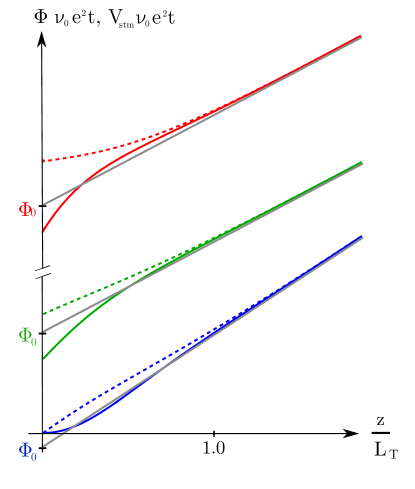
Figure 4: (color online) The spatial variation of the gauge-invariant potential $\Phi$ (solid lines) and the compensating voltage $V_{stm}$ at the STM tip (dashed lines) on the dimensionless distance $z/L_{T}$ from the boundary is plotted at different temperatures; $L_{t}/L_{T}=0.01$ (blue), $L_{t}/L_{T}=1$ (green) and $L_{t}/L_{T}=5$ (red). The solid grey lines represent the large distance asymptotes of the gauge invariant potential. Their intercepts with the vertical axis for the three values of $L_{t}/L_{T}$ are marked by $\Phi_{0}$ in the corresponding color. The value of $\Phi_{0}$ defines the junction resistance $R_{\infty}$ in Eq. (78).

One of the important features of transport through the junction is that at low temperatures the gauge invariant potential $\Phi(z)$ is significantly suppressed near the superconductor-normal metal boundary, and is a non-linear functions of $z$. In particular, the voltage drop across the insulator, $\Phi(z=0)$, goes to zero in the low temperature limit.

Because of the nontrivial spatial distribution of the electric field in the junction its resistive properties may be characterized in different ways. One measure of the resistance can be defined in terms of the voltage drop across the insulating barrier. We define the resistance of the insulating boundary per unit area as

$$R_{0}=\frac{\Phi(z=+0)}{J_{0}}.$$ (75)

Using Eq. (74) one can expression the boundary resistance $R_{0}$ per unit area in the form

$$R_{0}=\frac{1}{e^{2}\nu_{0}t}\frac{L_{t}}{L_{T}}A\left(\frac{L_{t}}{L_{T}}\right),$$ (76)

where the dimensionless function $A\left(L_{t}/L_{T}\right)$ is defined by the following integral

$$A\left(\frac{L_{t}}{L_{T}}\right) = \frac{L_{T}}{L_{t}}\int_{0}^{\infty}\frac{d\epsilon}{4T}\frac{\cot\theta_{R}(\epsilon,0)}{\cosh^{2}\frac{\epsilon}{2T}}.$$ (77)

This function is plotted in Fig. 5. In low and high temperature limits this expression tends to the following constants; $A(0)\approx 0.37$ and $A(\infty)\approx 0.53$. As a result in the high and low temperature regimes the boundary resistance $R_{0}\propto\sqrt{T}$.

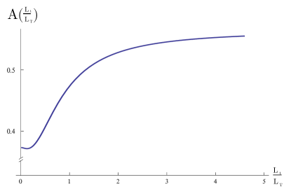
Figure 5: Plot of the function $A(L_{t}/L_{T})$ in Eqs. (76), (77).

Note that at low temperatures, $L_{T}\gg L_{t}$, the magnitude of the jump of $\Phi(z)$ at the insulator boundary approaches zero at $T\to 0$. This is very different from the resistance of the normal metal-insulator-normal metal junctions where in the presence of a current though the junction $R_{NIN}=1/e^{2}\nu_{0}\tilde{t}$, where $\tilde{t}\sim t_{0}^{2}$ is the transmission coefficient of the insulator.

Another measure of the junction resistance may be obtained by extrapolating the linear dependence of $\Phi(z)$ at large distances, $\Phi(z)=J_{0}z/\sigma_{D}+\Phi_{0}$ to the location of the barrier, $z=0$. This is shown by grey solid lines in Fig.  4. The value of the intercept with the vertical axis, $\Phi_{0}$, defines the total resistance per unit area of the junction

$$R_{\infty}=\frac{\Phi_{0}}{J_{0}}.$$ (78)

Using Eq. (74) we obtain

$$R_{\infty}=\frac{1}{e^{2}t\nu_{0}}B\left(\frac{L_{t}}{L_{T}}\right),$$ (79)

where the function $B(L_{t}/L_{T})$ is given by the following integral

$$B=\int_{0}^{\infty}\frac{d\epsilon}{2T}\frac{1}{\cosh^{2}\frac{\epsilon}{2T}}\left[\frac{1}{2\Gamma_{\epsilon}}-\int_{0}^{\infty}\frac{dz^{\prime}}{L_{t}}\tanh^{2}\theta_{I}(\epsilon,z^{\prime})\right].$$ (80)

The first term in the brackets is positive and represents the contribution of the insulating boundary. The second term is negative. It describes the reduction of the resistance of the normal metal due to the proximity effect.

The junction resistance $R_{\infty}$ is plotted in Fig. (6) as a function of $L_{t}/L_{T}$. At relatively high temperatures $L_{t}/L_{T}\gg 1$, junction resistance $R_{\infty}$ is dominated by the contribution from the insulating boundary (first term in Eq. (80)). In this case $B(L_{t}/L_{T})\approx 0.53\,L_{t}/L_{T}$, in agreement with the discussion below Eq. (77). In the low temperature regime, $L_{t}\ll L_{T}$, the junction resistance is dominated by the change in the resistance of the normal metal due to the proximity effect (second term in Eq. (80) and becomes negative. In this case the junction resistance reduces to

$$R_{\infty}=-\frac{b}{e^{2}t\nu_{0}}\frac{L_{T}}{L_{t}},$$ (81)

where the constant $b$ is given by

$$b = \int_{0}^{\infty}\frac{d\lambda}{2}\frac{\lambda^{-1/2}}{\cosh^{2}\frac{\lambda}{2}}$$ (82)

$$\times\int_{0}^{\infty}d\zeta\tanh^{2}\left[4\,\mathrm{Im}\arctan\left((\sqrt{2}-1)e^{(i-1)\zeta}\right)\right]$$

$$\approx 0.39.$$

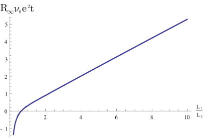
Figure 6: The junction resistance $R_{\infty}$ per unit area (in units of $1/e^{2}\nu_{0}t$) is a plotted as a function of $L_{t}/L_{T}$.

III.1 Probing the spatial distribution of the gauge-invariant potential $\Phi(\mathbf{r})$

Let us now discuss the possibility of experimental observation of the suppression of $\Phi(x)$ near the junction’s boundary by using a scanning tunneling probe. We consider the setup illustrated in Fig. 1.

The electron transport between the STM tip and the metal can be described with the aid of the tunneling Hamiltonian

$$H_{T}=\sum_{\mathbf{k}\mathbf{p}}\left[t_{\mathbf{kp}}c_{\mathbf{k}}^{\dagger}c_{\mathbf{p}}+t_{\mathbf{kp}}^{*}c_{\mathbf{p}}^{\dagger}c_{\mathbf{k}}\right].$$ (83)

Here $c^{\dagger}$ is an electron creation operator, and $\mathbf{k}$ labels the states in the STM tip and $\mathbf{p}$ labels the states in the wire. In the tunneling approximation the STM current can be written in the form

$$I_{stm}(z) = \frac{g_{n}}{2e}\int_{-\infty}^{\infty}d\epsilon\cos\theta_{R}(\epsilon,z)\cosh\theta_{I}(\epsilon,z)$$ (84)

$$\times\left[f_{1}^{stm}(\epsilon)-f_{1}(\epsilon,z)\right],$$

where $g_{n}$ is the conductance of the tunneling contact in the normal state. The nonequilibrium distribution function in the STM is given by $f_{1}^{stm}(\epsilon)=eV_{stm}/2T\cosh^{2}(\epsilon/2T)$, where $V_{stm}$ is the STM voltage measured relative to that in the superconductor.

Using Eq. (49) we can rewrite Eq. (84) in the form

$$I_{stm}(z)=g_{n}\Phi(z)-g_{t}(T,z)V_{stm},$$ (85)

where

$$g_{t}(T,z)=g_{n}\int_{0}^{\infty}\frac{d\epsilon}{2T}\frac{\cos\theta_{R}(\epsilon,z)\cosh\theta_{I}(\epsilon,z)}{\cosh^{2}\frac{\epsilon}{2T}}$$ (86)

is the conductance of the tunneling contact.

In the case where the voltage $V_{stm}$ at the tip vanishes the value of the tunneling current through the STM contact is proportional to $\Phi(z)$,

$$I_{stm}(z)=g_{n}\Phi(z).$$ (87)

In particular, $I_{stm}(z)$ is significantly suppressed near the superconductor-normal metal boundary, reflecting corresponding suppression of $\Phi(x)$.

On the other hand, if $I_{stm}=0$, we get

$$V_{stm}(z)=\frac{g_{n}}{g_{t}(T,z)}\,\Phi(z),$$ (88)

where $\Phi(z)$ is given by Eq. (74). The graph of $V_{stm}(z)$ is plotted in Fig. 4 by dashed lines for several temperatures. It is interesting to note that, in contrast to the gauge invariant potential, Eq. (87), the compensating STM voltage in Eq. (88) does not exhibit the aforementioned suppression near the boundary at low temperatures, $L_{T}\gg L_{t}$. The slope $dV_{stm}(z)/dz$ remains practically the same as in the normal metal in the absence of superconductor, both at $z\ll L_{T}$ and at $z\gg L_{T}$. The reason is that the conductance of the tunneling barrier between the STM and the metal, $g_{t}(T,z)$, reflects the suppression of the single particle density of states in the metal, as described by Eq. (86). This nearly cancels the suppression of $\Phi(z)$ in Eq. (88).

IV Conclusions

We show that the low temperature resistance of the p-wave superconductor-diffusive normal metal junctions is controlled by the spin-orbit interaction. As a result the junction resistance, tunneling density of states in the metal and other transport properties of the device exhibit a strong dependence on the angle between the vector ${\bf d}$ characterizing the spin part of the superconducting wave function, and the normal to the surface of the junction. In particular, the s-wave component of the proximity effect in metal vanishes when ${\bf d}$ is parallel to the c-axis.

The absence of the corresponding dependence of the Knight shift on the angle between ${\bf d}$ and the c-axis in $Sr_{2}RuO_{4}$ crystals is one of the problems in the interpretation of $Sr_{2}RuO_{4}$ as a conventional p-wave superconductor. This fact was attributed to weakness of the spin-orbit interaction in $Sr_{2}RuO_{4}$.knight We would like to point out that the resistance of the junction should be strongly dependent on the angle between ${\bf d}$ and ${\bf z}$ even in the case of weak spin-orbit interaction. Therefore the measurement of this effect could clarify the situation.

Another consequence of the sensitivity of the proximity effect to the orientation of the condensate spin is that a current passing across such a junction leads to spin accumulation inside the p-wave superconductor (although inside the proximity region no spin accumulation occurs).

We also would like to mention that the boundary conditions Eq. (60) can be used to describe the Josephson effect in junctions consisting of two p-wave superconductors separated by a diffusive normal metal. The structure of boundary conditions (60) is similar to those of for s-wave superconductor-normal metal junction. Therefore the supercurrent for the p-wave case may be obtained from the conventional formulas for the s-wave case if we substitute the phase difference in the s-wave case with $\phi_{\mathbf{d}}+\chi_{0}$, see Eqs. (59) and (55), and the transmission coefficient with $t$.

An important consequence of the proximity effect near the superconductor-normal metal boundary is the suppression of the Hall effect in the metal near the superconducting boundary. Qualitatively, this suppression is related to the fact that, due to proximity effect, at low energies the quasiparticle wave functions in metal are a coherent superposition of electron and hole wave functions, and the effective charge of the quasiparticles approaches zero at $\epsilon\rightarrow 0$. The presented above scheme of calculation of the electronic transport was derived in zeroth order in $\omega_{c}\tau$, where $\omega_{c}$ is the cyclotron frequency and $\tau$ is the elastic mean free time. In this approximation the electron wave functions near the Fermi surface are electron-hole symmetric, which yields a vanishing Hall effect. To describe Hall effect one has to add to the expression for the current a term linear in $\omega_{c}\tau$,ZhouSpivak

$$\mathbf{J}_{H}\propto\omega_{c}\tau{\bf b}\times\int d\epsilon\cos\theta_{R}\cosh^{3}\theta_{I}\bm{\nabla}f_{1}$$ (89)

here $\omega_{c}$ is the cyclotron frequency, and ${\bf b}$ is the unit vector in the direction of the magnetic field. Since the magnitude of the proximity effect is controlled by $t$, which is proportional to $\sin\vartheta_{\mathbf{d}}$, the Hall conductance is expected to have a strong dependence on the orientation of the order parameter, $\mathbf{d}$. Since the latter may be oriented by the external magnetic field, both the magnetoresistance of the junction and the Hall resistance are expected to be strongly anisotropic with respect to orientation of the magnetic field.

Finally, we note that our results hold for more general realizations of $p_{x}+ip_{y}$ order parameter in superconductors with complicated topology of the Fermi surface, such as the one proposed in Ref. kivelson, .

This work was supported by the US Department of Energy through the grant DE-FG02-07ER46452. B. S. thanks the International Institute of Physics (Natal, Brazil) for hospitality during the completion of the paper.

References

- (1) G. M. Blonder, M. Tinkham, and T. M. Klapwijk, Phys. Rev. B, 25 4515 (1892).
- (2) F. W. J. Hekking and Yu. V.Nazarov, Phys. Rev. B, 49, 6847 (1994).
- (3) T. H. Stoof and Yu. V. Nazarov, Phys. Rev. B, 53, 14496 (1996).
- (4) C. W. J. Beenakker, Phys. Rev. B, 46, 12841 (1992).
- (5) C. W. J. Beenakker, Rev. Mod. Phys., 69, 731 (1997).
- (6) F. Zhou, B. Spivak, and A. Zyuzin, Phys. Rev. B, 52, 4467 (1995).
- (7) Nelson, K. D. and Mao, Z. Q. and Maeno, Y. and Liu, Y., Science, 306, 1151 (2004).
- (8) Francoise Kidwingira, J. D. Strand, D. J. Van Harlingen, and Yoshiteru Maeno, Science, 314, 1267 (2006).
- (9) Xia, Jing and Maeno, Yoshiteru and Beyersdorf, Peter T. and Fejer, M. M. and Kapitulnik, Aharon, Phys. Rev. Lett. 97, 167002 (2006).
- (10) G. M. Luke at al., Nature 394, 558 (1998).
- (11) A. P. Mackenzie and Y. Maeno, Rev. Mod. Phys., 75, 657 (2003).
- (12) Y. Maeno, S. Kittaka, T. Nomura, S. Yonezawa, and K. Ishida, J. Phys. Soc. of Japan, 81, 011009 (2012).
- (13) J. Xia, Y. Maeno, Yoshiteru, P. T. Beyersdorf, M. M. Fejer, and A. Kapitulnik, Phys. Rev. Lett., 97, 167002 (2006).
- (14) T. M. Rice and M. Sigrist, J.Phys.: Condens. Matter 7, L613 (1996).
- (15) P. W. Anderson, and P. Morel, Phys.Rev. 123, 1911, (1961).
- (16) S. Raghu, A. Kapitulnik, and S. A. Kivelson, Phys. Rev. Lett., 105, 136401 (2010).
- (17) S. Kashiwaya et al., Phys. Rev.Lett. 107, 077003 (2011).
- (18) Laube, F. and Goll, G. and Löhneysen, H. v. and Fogelström, M. and Lichtenberg, F., Phys. Rev. Lett. 84, 1595, (2000).
- (19) Liu, Y. and Nelson, K.D. and Mao, Z.Q. and Jin, R. and Maeno, Y., J. Low. Temp. Phys. 131, 1059 (2003).
- (20) Kirtley, J. R. and Kallin, C. and Hicks, C. W. and Kim, E.-A. and Liu, Y. and Moler, K. A. and Maeno, Y. and Nelson, K. D., Phys.Rev. B 76, 014526 (2007).
- (21) C. Kallin, Rep. Prog. Phys., 765, 042501 (2012).
- (22) V. P. Mineev, and K. V. Samokhin, Introduction to unconventional superconductivity, Amsterdam, Gordon and Breach Science Publishers, (1999).
- (23) H. Murakawa, K. Ishida, K. Kitagawa, Z. Q. Mao, and Y. Maeno, Phys. Rev. Lett., 93, 167004 (2004).
- (24) A. I. Larkin, and Yu. N. Ovchinnikov,, Sov. Phys. JETP 41 960 (1975) ; Sov. Phys. JETP 46, 155 (1977).
- (25) A. L. Shelankov, J. Low Temp. Phys. 60, pg. 29-44, (1985).
- (26) A. V. Zaitsev, Sov. Phys. JETP, 59, 1015 (1984).
- (27) A. Millis, D. Rainer, and J. A. Sauls, Phys. Rev. B, 38, 4504 (1988).
- (28) M. Y. U. Kuprianov and V. F. Lukichev, Sov. Phys. JETP, 67, 1163 (1990).
- (29) F. Zhou, and B. Spivak, Phys. Rev. Lett., 80, 3847 (1998).