Comparison of classical and quantal calculations of helium three-body recombination

Abstract

A general method to study classical scattering in $n$-dimension is developed. Through classical trajectory calculations, the three-body recombination is computed as a function of the collision energy for helium atoms, as an example. Quantum calculations are also performed for the $J^{\Pi}$ = $0^{+}$ symmetry of the three-body recombination rate in order to compare with the classical results, yielding good agreement for $E\gtrsim$ 1 K. The classical threshold law is derived and numerically confirmed for the Newtonian three-body recombination rate. Finally, a relationship is found between the quantum and classical three-body hard hypersphere elastic cross sections which is analogous to the well-known shadow scattering in two-body collisions.

I Introduction

True three-body collision processes (A+B+C) are vitally important in a number of physical and chemical contexts,Brown et al. (1994); Huang et al. (2012), yet theoretical studies have been far less extensive than the vast literature that exists for two-body entrance channels (AB+C). Classical trajectory methods are based on the assumption that the motion of each of the nuclei in a chemical systems is governed to a good approximation by the laws of classical mechanics on the quantal potential energy surface given by the adiabatic electronic energy of the system. These methods have been successfully applied to calculations of scattering observables (e.g. the differential cross section, the reaction probability and the integral or total cross section) in many different chemical systems, often showing good agreement with experimental results and with quantum calculations.Schneider et al. (1995); Aoiz et al. (1998, 2005) Perhaps surprisingly, the classical trajectory methods can in some cases describe demanding properties of the chemical systems, such as the kinetic isotope effect observed in muonic isotopologues of the H + H₂ reaction.Jambrina et al. (2011); Homayoon et al. (2012)

In general, the agreement between classical trajectory methods and quantum mechanical calculations deteriorates at lower collision energies, where a low number of partial waves contribute. One might imagine that this issue would prevent us from studying cold and ultracold collisions by means of classical trajectory methods. However, in these situations it is informative to capitalize on the intuitive framework provided by the classical trajectory methods to analyze the role of the quantum effects and compare with Newtonian predictions.

Recently, Li and HellerLi and Heller (2012) have applied classical trajectory calculations to simulate buffer-gas cooling experiments with helium atoms and large rigid asymmetric-top molecules at a temperature as cold as 6.5 K. That treatment enabled the authors to calculate the lifetimes of long-lived orbiting resonances associated with the motion of an atom around a large molecule.Li and Heller (2012) They also predict that the production of cold molecules could be made more efficient by increasing the density of the buffer-gas.Li and Heller (2012) This exemplifies the potential utility of classical trajectory calculations for understanding the collision dynamics, even for cold systems.

At the same time, different mechanisms have been postulated at different times for three-body recombination. One of these is direct three-body recombination, which is closest to the class of processes considered in the present work. A second class of mechanisms involves indirect or “two-step” pathways, in which two of the particles initially collide and form a transient resonant state of vibration and/or rotation, followed by a subsequent de-excitation of the resonant state into a bound dimer in a second collision between the dimer and a third atom. This second class has been considered extensively in the literature and there are a number of different versions of it depending on which degree of freedom is initially excited in the first resonant collision. It is variously termed the “Lindemann-Hinshelwood mechanism”, or when formulated more specifically for three-atom collisions, one frequently sees reference to this as the “RBC mechanism” after the authors Roberts, Bernstein, and Curtiss.Roberts et al. (1969); Orel (1987)

While a “direct” three-body recombination collision would seem to be fundamentally different from these two-step mechanisms, one study has claimed that all of the alternative three-body mechanisms are equivalent and should produce identical three-body recombination rate coefficients.Wei et al. (1997) The present study of helium three-body recombination can indirectly test this assertion, because the ⁴He dimer has only one bound state and no discernible resonances on the electronic ground state potential. Thus the Lindemann-Hinshelwood or RBC mechanism predicts a vanishing three-body recombination rate, whereas both the quantal and classical calculations presented below produce direct recombination rates at low energy that exceed $10^{-30}$cm⁶/s. It remains unclear how this might be reconciled with the conclusions of Wei et al. (1997). The long, scholarly study by Pack, Walker, and KendrickPack et al. (1998a) also raised doubt as to the practical applicability of this claimed equivalence of indirect versus direct mechanisms.

The continuing development of both classicalEsposito and Capitelli (2009) and nonperturbative quantum mechanical descriptionsColavecchia et al. (2003) of this fundamental process is also interesting in view of recent approximate theory that computes quantum mechanical ternary rates in various approximations. One such applicationForrey (2013, ) has recently been applied to the crucial astrophysical problem of hydrogen atom three-body recombination. The hydrogen results presented appear to represent the current state of the art for three-body recombination in this system, but the main approximation utilized in that study (an energy sudden approximation) should be assessed critically. To explore other theoretical studies of recombination or its time-reverse process (collision-induced dissociation, CID) and the validity of various approximation methods, see also Refs.Ivanov and Babikov (2012); Azriel et al. (2011); Charlo and Clary (2004); Xie et al. (2003); Bernshtein and Oref (2003); Karachevtsev and Vinogradov (1999); Pack et al. (1998a); Colavecchia et al. (2003); Parker et al. (2002); Pack et al. (1998b)

The present paper implements a general method to study classical collisions in $n$-dimensions. This method utilizes classical trajectory calculations to calculate the three-body recombination rate (TBRR) for helium atoms in a framework related to the pioneering formulation of F. T. Smith.Smith (1962) The collision treated range from ultracold energies 10^-4 K to the thermal range 10³ K. The classical calculations are compared with quantum results that we have computed for the TBRR in the $J^{\Pi}$=$0^{+}$ symmetry only. The quantum calculations are based on the combination of the adiabatic hyperspherical representationLin (1995); Esry et al. (1996) and the R-matrix method to obtain the scattering properties.Aymar et al. (1996) The Hamiltonian is represented in a discrete variable representation (DVR),Tolstikhin et al. (1996) with some modifications for a better description of the nonadiabatic couplings at short-range distances.Wang et al. (2011) Among the key results obtained are the classical threshold law for TBRR as a function of the collision energy and a relationship between the classical and quantum predictions for high collision energies. In particular, we find a result that can be interpreted as an $n$-dimensional generalization of the shadow scattering in two-body collisions.Child (1974); Levine (2005)

II Generalized classical scattering

This section presents our method for studying classical collisions in an arbitrary number of dimensions $n\geq 3$. This method emerges from a simple generalization to $n$-dimensions of the concepts necessary to formulate the scattering problem in classical mechanics, i.e. the impact parameter and the cross section. As an illustration of the method, the cross section for the hard-sphere model in $n$-dimensions is derived. This calculation generalizes the two-body hard-sphere collision formulas, an essential model that is useful for characterizing high energy collisions.

II.1 The method

In classical scattering, the collision between two particles can be seen in two equivalent ways: either a particle impinges upon a scattering center or two particles approach to each other with some interaction. After removing the ignorable center-of-mass (CM) motion and formulating the collision in the relative motion coordinate, the second situation is identical to the first one. This generalizes the notion of single particle scattering to $n$-dimensions. (For $N$ particles colliding in ordinary three-dimensional space in the absence of an external field, note that the total dimensionality of the collision is equal to $n=3N-3$.)

In a three-dimensional (3D) collision, a particle with a defined momentum moves towards a scattering center. The cross section for a collisional process is defined as the area drawn in a plane perpendicular to the initial momentum, which the relative motion of the particles needs to cross if a collision is to take place.Levine (2005) The impact parameter vector, $\vec{b}$, basically determines the scattering, and it is defined as the component of the vector position that lies in the plane perpendicular to the momentum before the collision.Levine (2005) Both the impact parameter vector and the scattering cross section are readly extended to the $n$-dimensional scattering. However, instead of dealing with a plane we must work with an $n-1$-dimensional hyperplane, perpendicular to the direction of the initial momentum.

Thus an integral over the impact parameter will be equivalent to the hyperarea of the hyperplane (in 3D we use the concept of area) perpendicular to the initial momentum. If one attaches the opacity function $\wp_{process}(\vec{b},\vec{P})$ that counts the number of trajectories that contribute to the specific collision process of interest (e.g. chemical reaction, elastic scattering, etc.), then the integral will give the hyperarea over such hyperplane weighted by those trajectories involved in the process, i.e. the cross section. It can be expressed as

$$\sigma_{process}(\vec{P})=\int\wp_{process}(\vec{b},\vec{P})d\Omega_{b}^{n-1}b^{n-2}db,$$ (1)

where $d\Omega_{b}^{n-1}$ is the differential solid angle element of the hyperangles of $\vec{b}$ and $n-1$ indicates the dimensionality of the hyperspace where $\vec{b}$ is defined. The opacity function, $\wp_{\rm{process}}(\vec{b},\vec{P})$ is the probability that a trajectory with particular initial conditions leads to the process under study. Classical trajectory calculations are performed in order to determine the opacity function, which is the key function required in order to obtain the cross section.

Eq. (1) yields the cross section for a particular orientation of the momentum, but the main quantity of interest in our present exploration is the cross section for a particular magnitude of the momentum, $P$. It is done by averaging Eq. (1) over the hyperangles associated with the momentum, i.e.,

$$\sigma_{\rm{process}}(P)=\frac{\int\wp_{\rm{process}}(\vec{b},\vec{P})d\Omega_{P}^{n}d\Omega_{b}^{n-1}b^{n-2}db}{\int d\Omega_{P}^{n}},$$ (2)

where $\Omega_{P}^{n}$ represents the hyperangles of the canonical mass-weighted momentum vector $\vec{P}$ in the $n$-dimensional space.

II.2 Hard-hypersphere collision in n-dimensions

This method is readily applied to a hard-sphere model collision in $n$-dimensions. We introduce the hard-hypersphere opacity function as

$$\wp_{\rm{hs}}(\vec{b},\vec{P})=\left\{\begin{array}[]{l l}1&\quad b\leq R_{0}.\\ 0&\quad b>R_{0}.\end{array}\right.$$ (3)

This expression of the opacity function is independent of the orientation of $\vec{b}$ and $\vec{P}$ (owing to the spherical symmetry of the model) and it only leads to a collision event when the magnitude of the impact parameter $b$ is less than a certain threshold distance $R_{0}$, the interaction radius of the hard-hypersphere.

Inserting Eq.(3) into Eq. (2), the cross section is expressed as

$$\sigma_{\rm{hs}}(P)=\int_{0}^{R_{0}}d\Omega_{b}^{n-1}b^{n-2}db=\Omega^{n-1}\frac{R_{0}^{n-1}}{n-1},$$ (4)

where $\Omega^{n-1}$ is the solid angle subtended by a $n-1$-dimensional sphere (in the geometrical sense). Taking into account the general expression for the solid angle for a $d$-sphere $\Omega_{d}=\frac{2\pi^{d/2}}{\Gamma(d/2)}$,Avery (1989) where $\Gamma$ is the Gamma function and $d$ represents the dimension of the sphere, we finally obtain

$$\sigma_{\rm{hs}}(P)=\frac{2\pi^{(n-1)/2}}{\Gamma(\frac{n-1}{2})}\frac{R_{0}^{n-1}}{n-1}.$$ (5)

Eq. (5) generalizes of the well-known expression of the cross section of the hard-sphere model in 3D, namely $\sigma=\pi R_{0}^{2}$, to $n$-dimension. To understand this relationship more deeply, one can visualize the circle as the intersection between a 3D sphere and a plane, and on the other hand the $n-1$-dimensional sphere is the intersection of an $n$-dimensional sphere and an $n-1$-dimensional hyperplane.

III Classical three-body recombination

The $n$-dimensional classical scattering method assisted by classical trajectory calculations is now implemented to calculate the TBRR for helium atoms as a function of the collision energy from ultracold energies, 10^-4 K, to thermal energies, 1000 K. The classical trajectory calculations consist of a detailed implementation of the ideas pioneered by Felix T. Smith,Smith (1962) with Monte Carlo (MC) sampling of trajectories used to calculate the opacity function and the three-body recombination cross section (TBRCS), which leads to the TBRR as is explained in this Section. The results we obtain by applying this $n$-dimensional classical scattering method to three-body collisions include the classical ultracold threshold law for TBRR as a function of the collision energy. Another result that emerges is the relationship between the classical and quantum elastic three-body cross sections, resulting in an expression similar to the shadow scattering present in two-body collision.Child (1974); Levine (2005)

III.1 The equations of motion

Next consider the classical scattering of three particles. Their motion of three particles in a potential energy landscape, $V(\vec{r}_{1},\vec{r}_{2},\vec{r}_{3})$ is governed by the Hamiltonian

$$H=\frac{\vec{p}_{1}^{2}}{2m_{1}}+\frac{\vec{p}_{2}^{2}}{2m_{2}}+\frac{\vec{p}_{3}^{2}}{2m_{3}}+V(\vec{r}_{1},\vec{r}_{2},\vec{r}_{3}),$$ (6)

where $\vec{p}_{i}$ and $\vec{r}_{i}$ represent the momentum and the vector position of the $i^{th}$ particle, respectively. In order to simplify the Hamiltonian we introduce the Jacobi coordinates (see Fig.1) defined by the relations

$$\vec{\rho}_{1} = \vec{r}_{2}-\vec{r}_{1},$$ (7a)

$$\vec{\rho}_{2} = \vec{r}_{3}-\frac{m_{2}\vec{r}_{2}+m_{1}\vec{r}_{1}}{m_{1}+m_{2}},$$ (7b)

$$\vec{\rho}_{CM} = \frac{m_{1}\vec{r}_{1}+m_{2}\vec{r}_{2}+m_{3}\vec{r}_{3}}{M},$$ (7c)

where $M=m_{1}+m_{2}+m_{3}$ is the total mass of the system. The transformation between Cartesian coordinates and Jacobi ones is a contact transformation.Whittaker (1937) The three-body Hamiltonian can be expressed in the Jacobi coordinates as Karplus et al. (1965)

$$H=\frac{\vec{P}_{1}^{2}}{2m_{12}}+\frac{\vec{P}_{2}^{2}}{2m_{3,12}}+\frac{\vec{P}_{\rm{CM}}^{2}}{2M}+V(\vec{\rho}_{1},\vec{\rho}_{2}),$$ (8)

where $\frac{1}{m_{12}}=\frac{1}{m_{1}}+\frac{1}{m_{2}}$; $\frac{1}{m_{3,12}}=\frac{1}{m_{3}}+\frac{1}{m_{1}+m_{2}}$; $V(\vec{\rho}_{1},\vec{\rho}_{2})$ is the potential energy expressed in terms of the Jacobi coordinates, which explicitly exhibits its lack of dependence on the center of mass (CM) coordinates, as expected, since the CM momentum is a constant of motion. $\vec{P}_{1}$, $\vec{P}_{2}$ and $\vec{P}_{\rm{CM}}$ are the canonical momenta that are conjugate to $\vec{\rho}_{1}$, $\vec{\rho}_{2}$ and $\vec{\rho}_{CM}$, respectively. Finally, omission of the trivial CM motion gives

$$H=\frac{\vec{P}_{1}^{2}}{2m_{12}}+\frac{\vec{P}_{2}^{2}}{2m_{3,12}}+V(\vec{\rho}_{1},\vec{\rho}_{2}).$$ (9)

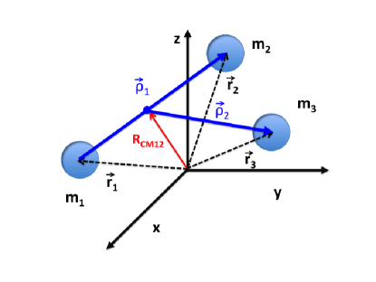
Figure 1: (Color online) Jacobi vectors for the three-body problem

The Hamilton equations of motion for the three particles as a function of the Jacobi coordinates are

$$\frac{d\rho_{i,\alpha}}{dt} = \frac{\partial H}{\partial P_{i,\alpha}},$$ (10a)

$$\frac{dP_{i,\alpha}}{dt} = -\frac{\partial H}{\partial\rho_{i,\alpha}},$$ (10b)

where $i=1,2$ and $\alpha=x,y,z$ in relation with the Cartesian coordinates of each Jacobi vector. The derivatives respect to $\rho_{i,\alpha}$ should be evaluated by taking into account Eqs. (7a), (7b) and (7c), combined with the chain rule. The solution of Hamilton’s equations determines the position of each particle as a function of time in the usual 3D space. In the usual manner Smith (1962) a 6D position vector is constructed form the two Jacobi vectors $\vec{\rho}_{1}$ and $\vec{\rho}_{2}$ as

$$\vec{\rho}=\begin{pmatrix}\vec{\rho}_{1}\\ \vec{\rho}_{2}\end{pmatrix}.$$ (11)

Hereafter, 6D vectors are represented in hyperspherical coordinates. The mass-scaled 6D canonical momentum vector can be written as

$$\vec{P}=\begin{pmatrix}\sqrt{\frac{\mu}{m_{12}}}\vec{P}_{1}\\ \sqrt{\frac{\mu}{m_{3,12}}}\vec{P}_{2}\end{pmatrix},$$ (12)

where $\mu=\sqrt{\frac{m_{1}m_{2}m_{3}}{M}}$. Now that the position vector and the momentum in a 6D space have been defined, the concept of impact parameter as the projection of the position vector in a hyperplane perpendicular to the initial momentum is clear. And, the three-body Hamiltonian is expressed as

$$H=\frac{\vec{P}^{2}}{2\mu}+V(\vec{\rho}).$$ (13)

In the present study, the TBRCS for helium atoms has been calculated with the three-body interaction approximated as the pairwise sum of helium dimer potentials, i.e.,

$$V(\vec{r}_{1},\vec{r}_{2},\vec{r}_{3})=v(r_{12})+v(r_{23})+v(r_{31}),$$ (14)

where $r_{ij}$ are the interparticle distances. This is not an essential aspect of the method, however, and it is possible for future studies to complete these calculations using a full three-body potential energy surface. In particular these calculations adopt the helium atom-atom interaction of Aziz et al., designated HFD-B3-FCI1Aziz et al. (1995), which has been tested on measurements of the transport coefficients and the second order virial coefficient, with demonstrated accuracy in the predictions of this interaction potential.

The equations of motion, Eqs. (10a) and (10b) are solved by means of an adaptative stepsize Runge-Kutta method, the Cash-Karp Runge-Kutta method.Press et al. (1986) The time stepsize varies from 10^-7 ns in regions where the atomic interaction varies steeply, up to 10^-4 ns in regions where the interaction varies smoothly. The total energy is conserved during collisions to at least four significant digits and the total angular momentum, $J=|\vec{\rho}_{1}\times\vec{P}_{1}+\vec{\rho}_{2}\times\vec{P}_{2}|$ is conserved to at least six digits.

III.2 Initial conditions

The equations of motion derived from the Hamilton’s equations determine the time evolution of all the dynamical variables of the system under study, those depend on their initial conditions. Indeed, the selection of the initial conditions is a crucial step in order to characterize the scattering properties through the concept of impact parameter as we have seen in Sec. II.

The scattering of three particles can of course alternatively be viewed as the scattering of one particle in 6 -dimensions. The 6-dimensional vectors are represented in a hyperspherical coordinate system based on the Avery’s definition of the hyperangles,Avery (1989) in this representation all the vectors can be represented by means of their magnitude $r$ and five different hyperangles ($\alpha_{i}$, $i=1,2,3,4,5$) by

$$\vec{r}=\begin{pmatrix}\vec{r}_{x_{1}}\\ \vec{r}_{x_{2}}\\ \vec{r}_{x_{3}}\\ \vec{r}_{x_{4}}\\ \vec{r}_{x_{5}}\\ \vec{r}_{x_{6}}\end{pmatrix}=\begin{pmatrix}r\sin{\alpha_{1}}\sin{\alpha_{2}}\sin{\alpha_{3}}\sin{\alpha_{4}}\sin{\alpha_{5}}\\ r\cos{\alpha_{1}}\sin{\alpha_{2}}\sin{\alpha_{3}}\sin{\alpha_{4}}\sin{\alpha_{5}}\\ r\cos{\alpha_{2}}\sin{\alpha_{3}}\sin{\alpha_{4}}\sin{\alpha_{5}}\\ r\cos{\alpha_{3}}\sin{\alpha_{4}}\sin{\alpha_{5}}\\ r\cos{\alpha_{4}}\sin{\alpha_{5}}\\ r\cos{\alpha_{5}}\end{pmatrix}.$$ (15)

Here the angle ranges are $0\leq\alpha_{1}\leq 2\pi$, $0\leq\alpha_{i}\leq\pi$, $i=2,3,4,5$. In particular, we choose to align the 3D $z$ axis parallel to $\vec{p}_{2}$, whereby the initial momentum $\vec{P}_{0}$ is expressed as [see Eq. (12)]

$$\vec{P}_{0}=\begin{pmatrix}P_{0}\sin{\alpha^{P}_{1}}\sin{\alpha^{P}_{2}}\sin{\alpha^{P}_{5}}\\ P_{0}\cos{\alpha^{P}_{1}}\sin{\alpha^{P}_{2}}\sin{\alpha^{P}_{5}}\\ P_{0}\cos{\alpha^{P}_{2}}\sin{\alpha^{P}_{5}}\\ 0\\ 0\\ P_{0}\cos{\alpha^{P}_{5}}\end{pmatrix},$$ (16)

where $0\leq\alpha^{P}_{1}\leq 2\pi$, $0\leq\alpha^{P}_{2}\leq\pi$ and $0\leq\alpha^{P}_{5}\leq\pi$. The impact parameter $\vec{b}$ is defined in a 5-dimensional hyperplane orthogonal to $\vec{P}_{0}$. It is a 5-dimensional vector embedded in a 6-dimensional space by means of the Avery’s hyperangle definition as

$$\vec{b}=\begin{pmatrix}b\sin{\alpha^{b}_{1}}\sin{\alpha^{b}_{2}}\sin{\alpha^{b}_{3}}\sin{\alpha^{b}_{4}}\\ b\cos{\alpha^{b}_{1}}\sin{\alpha^{b}_{2}}\sin{\alpha^{b}_{3}}\sin{\alpha^{b}_{4}}\\ b\cos{\alpha^{b}_{2}}\sin{\alpha^{b}_{3}}\sin{\alpha^{b}_{4}}\\ b\cos{\alpha^{b}_{3}}\sin{\alpha^{b}_{4}}\\ b\cos{\alpha^{b}_{4}}\\ 0\end{pmatrix},$$ (17)

where $0\leq\alpha^{b}_{1}\leq 2\pi$, $0\leq\alpha^{b}_{i}\leq\pi$, $i=2,3,4$.

The magnitude of the initial vector position $|\vec{\rho}_{0}|=R$ is chosen to ensure that the interaction potential is negligible at that point and beyond. Then Eq. (13) yields the magnitude of the initial momentum $E=P_{0}^{2}/2\mu$, with $E$ the collision energy, that is equal to the kinetic energy initially. Our procedure randomly generates different angles $\alpha^{P}_{i}$ with $i=1,2,5$, and $\alpha^{b}_{j}$ with $j=1,2,3,4$, for a particular magnitude of the impact parameter $|\vec{b}|$. Those angles are generated by means of the probability density function (PDF) associated with each of them, as is show in Sec. III.3. As the initial momentum $\vec{P}_{0}$ and the impact parameter $\vec{b}$ are orthogonal, the initial vector position can be written as

$$\vec{\rho}_{0}=\vec{b}-\frac{\sqrt{R^{2}-b^{2}}}{P_{0}}\vec{P}_{0}.$$ (18)

Eq. (18) now generates $\vec{\rho}_{0}$ from $R$, $\vec{b}$ and $\vec{P}_{0}$.

Note that the definition of the hyperradius used in this Newtonian part of the study differs from the choice of the hyperradius in the quantum calculations. For the classical treatment, no mass-scaling of the Jacobi coordinate vectors is carried out, whereas that scaling is uniformly implemented in all quantum calculations, e.g. those of this paper and in Refs. Esry et al. (1999); Suno et al. (2002); Wang et al. (2011, 2012)

III.3 The opacity function, probability of recombination, and three-body recombination rate

The average generalized cross section for the three-body collision is given by (Eq. 2 with $n$ = 6)

$$\sigma_{\rm{rec}}(P_{0})=\frac{\int\wp_{\rm{rec}}(\vec{b},\vec{P_{0}})b^{4}dbd\Omega_{b}d\Omega_{P_{0}}}{\int d\Omega_{P_{0}}},$$ (19)

This expression explicitly averages over all initial momentum directions and implies an average over the relative kinetic energies associated with the two initial Jacobi vectors. It takes into account the relationship between the initial momentum magnitude, $P_{0}$, and the collision energy, $E$, given in Sec. III.2. $\wp_{\rm{rec}}(\vec{b},\vec{P_{0}})$ is the three-body recombination opacity function, which is a function of all the collisional parameters: $b$, $\Omega_{b}$, $P_{0}$ and $\Omega_{P_{0}}$. $\Omega_{b}$ and $\Omega_{P_{0}}$ represent the hyperangles associated to the vectors $\vec{b}$ and $\vec{P_{0}}$, respectively. $d\Omega_{b}$ and $d\Omega_{P_{0}}$ are the differential element of the hyperangles of each vector. In particular, the Avery hyperangle definition Avery (1989) gives the following:

$$d\Omega_{b}=\sin^{3}{(\alpha^{b}_{4})}\sin^{2}{(\alpha^{b}_{3})}\sin{(\alpha^{b}_{2})}d\alpha^{b}_{4}d\alpha^{b}_{3}d\alpha^{b}_{2}d\alpha^{b}_{1},$$ (20)

and

$$d\Omega_{P_{0}}=\sin^{4}{(\alpha^{P_{0}}_{5})}\sin{(\alpha^{P_{0}}_{2})}d\alpha^{P_{0}}_{5}d\alpha^{P_{0}}_{2}d\alpha^{P_{0}}_{1},$$ (21)

These expressions take into account the fact that we have chosen the $z$ axis parallel to the $\vec{P}_{2}$ direction (see Sec. III.2).

The recombination trajectories are of course those trajectories that lead to the formation of bound dimers. In classical trajectory methods, the states of the dimer at positive energies, which would be called shape resonances in a quantum calculation, appear to be truly bound dimers. Some decisions must be made as to how to take into account the influence of such states that we know are actually quantum mechanical shape resonances having finite lifetimes.Roberts et al. (1969); Orel (1987); Esposito and Capitelli (2009) However, in the case of the helium dimer, we have checked by using the Wentzel-Kramers-Brillouin (WKB) approximation that the dimer interaction does not support any bound or quasi-bound state for $l\geq 2$ (l is the orbital angular momentum), which confirms that there is no shape resonances that must be considered in the case of the helium three-body problem. Accordingly, the only events counted as recombination are those trajectories which lead to bound dimers whose energy is negative.

The opacity function, $\wp_{\rm{rec}}(\vec{b},\vec{P_{0}})$, also called the reaction probability, represents the probability that the reactants transform into the products at each value of the initial collisional parameters. Usually it is given just in terms of the impact parameter $b$, but in some systems one is interested in the studying the effect of the reactant alignment and orientation on the product formation, i.e. the stereodynamics of the reaction.Levine (2005) Since the present study is not investigating the explicit orientation dependence of the opacity function, the quantity we focus on as the probability of recombination (PR) $\wp_{\rm{rec}}(b,P_{0})$ as the average opacity function

$$\wp_{\rm{rec}}(b,P_{0})=\frac{\int\wp_{\rm{rec}}(\vec{b},\vec{P_{0}})d\Omega_{b}d\Omega_{P_{0}}}{\int d\Omega_{b}d\Omega_{P_{0}}}.$$ (22)

The integral in Eq. (22) is evaluated by means of the MC integration method,Yu. Schreiber (1966); Landau and Binder (2009) i.e. the initial hyperangles ($\alpha^{b}_{4},\alpha^{b}_{3},\alpha^{b}_{2},\alpha^{b}_{1},\alpha^{P_{0}}_{5},\alpha^{P_{0}}_{1},\alpha^{P_{0}}_{2}$) are sampled by means of their PDF given by the Eqs. (20) and (21), and then the function $\wp_{\rm{rec}}(b,P_{0})$ is averaged over the randomly sampled hyperangles. Concretely, we run $n_{\rm{tra}}(b,P_{0})$ for a given $b$ and $P_{0}$, then count the number of those trajectories that lead to recombination events, $n_{\rm{rec}}(b,P_{0})$, and finally the PR is calculated as

$$\wp_{\rm{rec}}(b,P_{0})\approx\frac{n_{\rm{rec}}(b,P_{0})}{n_{\rm{tra}}(b,P_{0})}\pm\delta(b,P_{0}).$$ (23)

Here $\delta(b,P_{0})$ is the statistical error. Since $\wp_{\rm{rec}}(b,P_{0})$ is a Boolean function, i.e. $<\wp^{2}_{\rm{rec}}(b,P_{0})>$ = $<\wp_{\rm{rec}}(b,P_{0})>$, the statistical error is given byTruhlar and Muckerman (1975)

$$\delta(b,P)=\frac{\sqrt{n_{\rm{rec}}(b,P_{0})}}{n_{\rm{tra}}(b,P_{0})}\sqrt{\frac{n_{\rm{tra}}(b,P_{0})-n_{\rm{rec}}(b,P_{0})}{n_{\rm{tra}}(b,P_{0})}},$$ (24)

which assumes a one standard deviation rule (68$\%$ confidence level) for the evaluation of the statistical error. This error criterion is assumed for all the classical results reported in the present work.

The three-body recombination cross section is expressed in terms of the PR as

$$\sigma_{\rm{rec}}(P_{0})=\Omega_{b}\int_{0}^{b_{\rm{max}}(P_{0})}\wp_{\rm{rec}}(b,P_{0})b^{4}db,$$ (25)

where $b_{\rm{max}}(P_{0})$ represents the maximum impact parameter that leads to a recombination process for a fixed $P_{0}$, in other words, for $b>b_{max}(P_{0})$ it is found that $\wp_{\rm{rec}}(b,P_{0})=0$. $\Omega_{\rm{b}}=\frac{8\pi^{2}}{3}$ is the solid hyperangle associated with $\vec{b}$. The three-body recombination cross section is calculated by integrating Eq. (25) using MC sampling of the magnitude of the impact parameter, $b$. Our sampling in $b$ uses the importance sampling method based on the weight function $e^{-b/r_{0}}$,Shui (1972, 1973) where $r_{0}$ denotes the range of the interaction (15 a₀ for helium dimer interaction). Then, Eq. (25) is written as

$$\sigma_{\rm{rec}}(P_{0}) = \frac{8\pi^{2}}{3}\int_{0}^{b_{\rm{max}}(P_{0})}e^{b/r_{0}}\wp_{\rm{rec}}(b,P_{0})e^{-b/r_{0}}b^{4}db=$$ (26)

$$= \beta\frac{{8\pi^{2}}}{3}\int_{0}^{b_{\rm{max}}(P_{0})}e^{b/r_{0}}\wp_{\rm{rec}}(b,P_{0})\rho(b)db$$

where $\rho(b)=\frac{e^{-b/r_{0}}b^{4}}{\beta}$ and $\beta=\int_{0}^{b_{\rm{max}}(P_{0})}\rho(b)db$. The importance sampling function establishes a particular weight to any recombination trajectory as a function of $b$. In practice, Eq. (26) is solved by sampling $b$, taking into account $\rho(b)$, and the initial impact parameter and momentum hyperangles ($\alpha^{b}_{4},\alpha^{b}_{3},\alpha^{b}_{2},\alpha^{b}_{1},\alpha^{P_{0}}_{5},\alpha^{P_{0}}_{2},\alpha^{P_{0}}_{1}$) by means of their PDF given by the Eqs. (20) and (21). After $N_{\rm{tra}}(P_{0})$ are computed and the number of recombination events, $N_{\rm{rec}}(P_{0})$ are counted, they are weighted by the (inverse of the) importance sampling function, and finally the TBRCS is calculated as

$$\sigma_{\rm{rec}}(P_{0})\approx\beta\frac{8\pi^{2}}{3}\frac{\sum_{i=1}^{N_{\rm{rec}}(P_{0})}e^{b_{i}/r_{0}}}{N_{\rm{tra}}(P_{0})}\pm\Delta(P_{0}),$$ (27)

Here $\Delta(P_{0})$ is the statistical error, given by

$$\Delta(P_{0})=\beta\frac{8\pi^{2}}{3}\sqrt{\frac{\frac{\sum_{i=1}^{N_{rec}(P_{0})}e^{2b_{i}/r_{0}}}{N_{\rm{tra}}(P_{0})}-\left(\frac{\sum_{i=1}^{N_{\rm{rec}}(P_{0})}e^{b_{i}/r_{0}}}{N_{\rm{tra}}(P_{0})}\right)^{2}}{N_{\rm{tra}}(P_{0})}}.$$ (28)

The TBRR as function of the collision energy is obtained by means of the TBRCS as

$$k_{3}(P_{0})=v\sigma_{\rm{rec}}(P_{0})=\frac{P_{0}}{\mu}\sigma_{\rm{rec}}(P_{0}),$$ (29)

where $P_{0}$ is the magnitude of the momentum in hyperspherical coordinates, which is related to the collision energy $E$ as shown in Sec.III.2. Observe that we do compute the TBRR as a thermal average taking into account the Maxwell-Boltzmann weights, indeed we calculate the TBRR as a function of the collision energy. The thermal averaging can be readily carried out whenever it is desired to compare with the experiments performed in thermal equilibrium.

III.4 The classical low energy threshold law for the three-body recombination rate

In quantum mechanics the existence of threshold laws for elastic and inelastic collisions in different types of collision, are very familiar, the so-called Wigner threshold laws. These threshold laws represent the general trend of the cross section for different processes as functions of the collision energy. In the classical two-body collisions between an ion and a neutral species, the Langevin cross section Levine (2005) can be viewed as a similar low energy threshold behavior that gives the energy dependence analytically. Next we show that it is possible to derive the threshold behavior of the three-neutral-body recombination rate as a function of the collision energy. In the low energy range where long range interactions are dominated by the van der Waals potential $V(R)\rightarrow C_{6}/r^{6}$. We define the maximum impact parameter $\tilde{b}_{\rm{max}}$ as the distance where the interaction potential is equal to the collision energy, i.e.

$$E=\frac{C_{6}}{\tilde{b}_{\rm{max}}^{6}}.$$ (30)

The derivation for the classical threshold law for low energy collisions assumes a rigid-sphere model for the low-energy classical collisions, i.e. such that for $b<\tilde{b}_{\rm{max}}$ the opacity function can be taken to be 1. The three-body recombination cross section can then be expressed as (in virtue of Eq. (25) )

$$\sigma_{\rm{rec}}(E)=\frac{8\pi^{2}}{3}\int_{0}^{\tilde{b}_{\rm{max}}(E)}b^{4}db\propto\tilde{b}^{5}_{\rm{max}}(E),$$ (31)

which has taken into account the relationship between the initial momentum and the collision energy (see Sec.III.2). By means of Eqs. (30), (31) and (29), and by incorporating the relationship between momentum and energy ($P\propto E^{1/2}$), finally we obtain

$$k_{3}(E)\propto E^{1/2}\frac{1}{E^{5/6}}=E^{-1/3}.$$ (32)

III.5 Three-body elastic collisions at high collision energies

The quantum mechanical three-body elastic cross section for distinguishable particles whose potential energy is short-ranged and depends on the hyperradius is given by

$$\sigma^{3B}=\frac{32\pi^{2}}{k^{5}}\sum_{\lambda}N_{\lambda}|e^{2\imath\delta_{\lambda}}-1|^{2}=\frac{32\pi^{2}}{k^{5}}4\sum_{\lambda}N_{\lambda}\sin^{2}{\delta_{\lambda}}.$$ (33)

In this expression $\delta_{\lambda}$ is the three-body scattering phase shift for a given value of $\lambda$, the eigenvalue of the squared grand angular momentum operator (see Sec. IV), $k$ is the wave vector defined as $E=\hbar^{2}k^{2}/2\mu$, and $N_{\lambda}$ is a numerical factor that takes into account the degeneracy associated with the grand angular momentum

$$N_{\lambda}=\frac{4+2\lambda}{4}\frac{(\lambda+3)!}{\lambda!3!}.$$ (34)

The summation in Eq. (33) is extended over all the values of $\lambda$ (partial waves). But owing to the finite range of the potential energy, $\delta_{\lambda}\rightarrow 0$ for high values of $\lambda$, and therefore the summation in practice has a finite number of terms. Interestingly, Eq. (33) exhibits a close similarity with the usual two-body classical cross section, where the summation is over the angular momentum $l$.Landau and Lifshitz (1958)

For a high energy collision a large number of partial waves must be included for the computation of the cross section. In general, at high energies the phase shift, $\delta_{\lambda}$, is a rapidly varying and effectively random function of $\lambda$, whereby the three-body elastic cross section of Eq. (33) is given by

$$\sigma^{3B}\approx\frac{32\pi^{2}}{k^{5}}2\sum_{\lambda=0}^{\lambda_{max}}N_{\lambda},$$ (35)

where $\lambda_{\rm{max}}$, it is the highest value of $\lambda$ satisfying the random phase criterion. Eq. (35) neglects contributions to the summation for $\lambda>\lambda_{\rm{max}}$. If $\lambda_{\rm{max}}>>1$ then

$$\sum_{\lambda=0}^{\lambda_{\rm{max}}}N_{\lambda}\approx\sum_{\lambda=0}^{\lambda_{\rm{max}}}\frac{\lambda^{4}}{12}\approx\frac{\lambda_{\rm{max}}^{5}}{5\times 12}.$$ (36)

Finally, the three-body elastic cross section is expressed as

$$\sigma^{3B}\approx\frac{16\pi^{2}}{3k^{5}}\frac{\lambda_{\rm{max}}^{5}}{5}.$$ (37)

The classical three-body elastic cross section is given by Eq. (19), where we have to include the right opacity function associated with the elastic collisions. For high energy collisions we assume a hard-sphere collision model [Eq. (3)]. Therefore, the cross section becomes

$$\sigma(P_{0})=\frac{8\pi^{2}}{3}\int_{0}^{R}b^{4}db=\frac{8\pi^{2}R^{5}}{3\times 5}.$$ (38)

The initial grand angular momentum is defined as

$$\vec{\Lambda}=\vec{\rho}_{0}\times\vec{P}_{0},$$ (39)

where the cross product is defined in a 6D space (i.e., the generalized cross product is defined in terms of the Levi-Civita tensor). Using the fact that $\vec{P}_{0}$ and $\vec{b}$ are orthogonal implies that

$$|\vec{\Lambda}|^{2}=b^{2}P_{0}^{2}.$$ (40)

The eigenvalues of the grand angular momentum are $\hbar^{2}\lambda(\lambda+4)$,Avery (1989) for high values of $\lambda$ which can be approximated by $\hbar^{2}\lambda^{2}$, thus Eq. (40) determines the relation between the partial wave scattering formulation and the impact parameter treatment. The result is

$$\lambda_{max}=kR.$$ (41)

Eq. (41) establishes a relationship between the quantum three-body elastic cross section, Eq. (37), and the classical Eq. (38) as

$$\sigma^{3B}=2\times\sigma(P_{0}).$$ (42)

In Eq. (42) we notice that the high energy collision limit of the quantum three-body elastic cross section is two times the classical one. This same factor of two also holds for two-body collisions and it is interpreted in terms of shadow scattering.Child (1974); Levine (2005) Thus, Eq. (42) implies the existence of shadow scattering in three-body collisions, and it counts for half of the cross section just as it does for two-body collisions.

IV Quantum three-body recombination

The present study extends the previous calculations of the TBRR for helium atoms by Suno et al.Suno et al. (2002) to higher collision energies. In particular, the present quantum calculations treat only the $J^{\Pi}$ = $0^{+}$ symmetry and these can be compared with Newtonian recombination rate contributions for collisions with less than one unit of angular momentum. A different method is employed for calculating the TBRR than was by of Suno et al. The Schrödinger equation is solved for three interacting helium atoms using a two steps method: first, the adiabatic potentials are computed by means a combination of slow variable discretization (SVD) method Tolstikhin et al. (1996) at short distances, and a traditional adiabatic hyperspherical representation for long distances, in particular, a DVR hyperradial basis is utilized whereas the b-splines method is employed for the hyperangles. Second, we apply R-matrix theoryAymar et al. (1996) for the calculation of the scattering properties.Wang et al. (2011)

The three-body scattering Hamiltonian is formulated in the modified Smith-Whitten hyperspherical coordinates:Suno et al. (2002) $\{R,\Omega\}\equiv\{R,\theta,\phi,\alpha,\beta,\gamma\}$. $R$ is the hyperradius and $\theta$ and $\phi$ are the hyperangles that describe the internal motion of the three-body system. In these hyperspherical coordinates the interparticle distances are expressed asSuno et al. (2002)

$$r_{12} = 3^{-1/4}R[1+\sin{\theta}\sin{(\phi-\pi/6)}]^{1/2},$$ (43a)

$$r_{23} = 3^{-1/4}R[1+\sin{\theta}\sin{(\phi-5\pi/6)}]^{1/2},$$ (43b)

$$r_{13} = 3^{-1/4}R[1+\sin{\theta}\sin{(\phi+\pi/2)}]^{1/2},$$ (43c)

and the three-body Schrödinger equation is given (in a.u.) by

$$\left[-\frac{1}{2\mu}\frac{\partial^{2}}{\partial R^{2}}+\frac{\Lambda^{2}+15/4}{2\mu R^{2}}+V(R,\theta,\phi)\right]\psi_{\nu^{\prime}}(R,\Omega)=$$ (44)

$$E\psi_{\nu^{\prime}}(R,\Omega).$$

where $\Lambda^{2}$ is the squared ”grand angular momentum operator”.Suno et al. (2002); Kendrick et al. (1999); Lepetit et al. (1990) $\psi_{\nu^{\prime}}=R^{5/2}\Psi_{\nu^{\prime}}$ is a rescaled version of the usual Schrödinger solution $\Psi_{\nu}$. The index $\nu^{\prime}$ labels the different independent solutions that are degenerate in energy and includes the quantum numbers that distinguish the degenerate states.Wang et al. (2011) The three-body interaction is taken here to be a sum of the three pairwise two-body helium interactions, based on the helium dimer potential of Aziz et al.Aziz et al. (1995), designated as HFD-B3-FCI1 (the same as we use for the classical calculations). Recently, Suno and Esry have performed quantum calculations on three-body recombination rate for helium atoms by using a potential energy surface including three-body electronic interactions.Suno and Esry (2008)

Eq. (44) is solved in the adiabatic hyperspherical representation for a given symmetry $J^{\Pi}$. The wave function is represented in terms of the complete, orthonormal set of angular wave functions $\Phi_{\nu}(R,\Omega)$ and radial wave functions $F_{\nu\nu^{\prime}}$ as

$$\psi_{\nu^{\prime}}(R,\Omega)=\sum_{\nu=1}^{Nc}F_{\nu\nu^{\prime}}(R,\Omega)\Phi_{\nu}(R,\Omega),$$ (45)

where $N_{c}$ indicates the number of channels in the adiabatic basis that we chose to represent the wave function. The channel functions $\Phi_{\nu}(R,\Omega)$ are eigenfunctions of the five-dimensional partial differential equation

$$\left[\frac{\Lambda^{2}+15/4}{2\mu R^{2}}+V(R,\theta,\phi)\right]\Phi_{\nu}(R,\Omega)=$$

$$U_{\nu}(R)\psi_{\nu}(R,\Omega),$$ (46)

whose solutions depend parametrically on R. Insertion of the wave function expression in terms of the adiabatic basis, Eq. (45), into the Schrödinger equation, Eq. (44), yields a set of coupled ordinary differential equations in $R$

$$\left[-\frac{1}{2\mu}\frac{d^{2}}{dR^{2}}+U_{\nu}(R)-E\right]F_{\nu\nu^{\prime}}(R)$$

$$-\frac{1}{2\mu}\sum_{\gamma=1}^{N_{c}}\left[2P_{\nu\gamma}(R)\frac{d}{dR}+Q_{\nu\gamma}(R)\right]F_{\gamma\nu^{\prime}}(R)=0.$$ (47)

The matrices $P_{\nu\gamma}(R)$ and $Q_{\nu\gamma}(R)$ denote the nonadiabatic couplings between the different adiabatic channels associated with the same symmetry. These matrices are defined as

$$P_{\nu\gamma}(R)=\int d\Omega\Phi_{\nu}(R,\Omega)^{*}\frac{\partial}{\partial R}\Phi_{\gamma}(R,\Omega),$$ (48)

and

$$Q_{\nu\gamma}(R)=\int d\Omega\Phi_{\nu}(R,\Omega)^{*}\frac{\partial^{2}}{\partial R^{2}}\Phi_{\gamma}(R,\Omega).$$ (49)

These nonadiabatic couplings are crucial in determining the inelastic transitions and the width of the resonances supported by the adiabatic potentials $U_{\nu}(R)$. Thus, we need to describe accurately such nonadiabatic couplings. In general, at short-range distances is where one would expect sharp nonadiabatic avoided crossings.

The solution of Eq. (IV) including effects of the nonadiabatic couplings is accomplished by means of the SVD method, which gives an efficient description of coupling effects.Wang et al. (2011) Instead in the long-range region, the adiabatic hyperspherical coupled equations are solved directly in the ordinary adiabatic representation using the $P,Q$ matrices, with a DVR basis set.Wang et al. (2011) This method is more practical at large $R$ where the nonadiabatic couplings are smooth functions of $R$. The computation of the nonadiabatic couplings outside of the SVD region applies the method proposed by Wang et al..Wang et al. (2012) In practice Eq. (IV) is solved from 1 $a_{0}$ to 35 $a_{0}$, for a set of 117 SVD sectors, in each of which 10 SVD points are utilized. Beyond that region, a DVR basis set is used in a variational R-matrix calculation with about 10⁵ sectors from 35 $a_{0}$ to 2x10⁴ $a_{0}$ for the calculation of the adiabatic potentials $U_{\nu}(R)$ and nonadiabatic couplings.

The scattering S matrix is extracted from the R-matrix method in the long-range region. Aymar et al. (1996) 30 adiabatic channels have been employed on the calculations. The solution of the adiabatic equations takes about 36 CPU hours using 16 processors in parallel and the solution of the coupled equations is about 3 CPU hours per energy.

As in previous references,Esry et al. (1999) the three-body cross section for three identical bosonic particles is defined using the convention of Mott and Massey,Mott and Massey (1965) in which the scattering cross section $\sigma_{3}$ is the ratio of the scattered radial flux multiplied by $R^{5}$ divided by the incident flux in only one of the six symmetrizing permutations of the incident plane wave.Esry et al. (1999); Mehta et al. (2009) The differential cross section is then integrated over all final hyperangles and averaged over the initial momentum hyperangles to get an average generalized recombination cross section. The total three-body recombination rate is then

$$K_{3}=\frac{k}{\mu}\sigma_{3}^{K}=\sum_{J,\Pi}K_{3}^{J\Pi},$$ (50)

where $K_{3}^{J\Pi}$ is the partial recombination rate corresponding to the $J^{\Pi}$ symmetry

$$K_{3}^{J\Pi}=\sum_{i,f}\frac{192\left(2J+1\right)\pi^{2}}{\mu k^{4}}|S_{i\rightarrow f}^{J\Pi}|^{2}.$$ (51)

Here $i$ and $f$ label the incident (three-body continuum) and outgoing (two-body recombination) channels, respectively, and $k=(2\mu E)^{1/2}$ are the hyperradial wave numbers in the incident channels. The helium dimer interaction has only one two-body recombination channel. Because the present study considers only the $J^{\Pi}=0^{+}$ symmetry, thus the in Eq. (50) this summation reduces to a single term.

V Results and discussion

The TBRR is computed as a function of the collision energy of helium atoms from ultracold energies up to thermal energies using both classical and quantum methods, and compared in the following.

The visualization of the classical trajectories helps to understand the physical mechanism controlling the recombination process being investigated. Fig. 2 shows two recombination trajectories at 10^-4 K for different impact parameters: null impact parameter (upper panel), and $b$ = 100 a₀ (lower panel). Observe that the collisions for different impact parameters lead to recombination trajectories with different final states of rotation and vibration of the bound dimers. Thus, the energy of the dimers associated with those trajectories will be different. We note that the trajectories with null impact parameter start to be deflected at distances where one of the interatomic distance has a small value. On the contrary, the trajectories at high impact parameter show a deflection before any interatomic distance start to be small. Fig. 2 shows that the three-body recombination events need at least two atom-atom collisions in order to form a bound dimer. It is instructive to introduce the three-body collision time, $\tau_{3}$, as the time from when the atoms first start to experience their interaction (i.e. as reflected by a change in the initial slope of the trajectory ) until the time when two atoms form a bound dimer. Analysis of Fig. 2 shows that the collision time is $\tau_{3}\sim 10$ ns at 10^-4 K. At 1000 K the three-body collision time for a characteristic trajectory is $\tau_{3}\sim 10^{-3}$ ns.

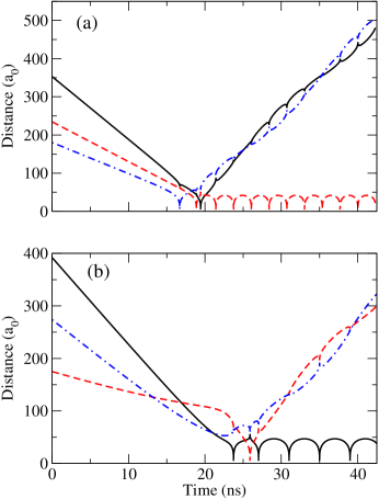
Figure 2: (Color online) Examples of recombination trajectories for E = 10^-4 K. Panel (a): classical trajectories for $b$=0 a₀. Panel (b), classical trajectories for $b$=100 a₀. The solid line represents $r_{12}$, the dashed line represents $r_{23}$ and the dot-dashed line represents $r_{31}$

The probability of recombination (PR) [$\wp_{\rm{rec}}(b,P)$] for helium atoms as a function of the impact parameter, at collisional energies: 10^-4 K, 10^-2 K, 1 K and 25 K, is presented in Fig. 3. The PR has been calculated following the method described in Sec. III.3. These results use an equally spaced grid in $b$, and for each of those $b$-values we run 10³ trajectories for the calculation of the PR [Eq. (23)] and its statistical error [Eq. (24)], i.e. $n_{\rm{tra}}(b,P_{0})=10^{3}$. From this figure the maximum impact parameter producing a recombination for a given energy, $b_{\rm{max}}$, is extracted, and this equals: 235 a₀, 120 a₀, 58 a₀ and 40 a₀, for 10^-4 K, 10^-2 K, 1 K and 25 K, respectively. We note a general trend for $E<1$ K: a reduction of $b_{\rm{max}}$ by a factor of two while the change in energy is two orders of magnitude. However, this trend for $b_{\rm{max}}$ changes for energies between 1 K and 25 K, where it exhibits a steep trend as a function of the collision energy. This suggests that a different dynamical regime starts to play a role for $E\gtrsim 1$ K.

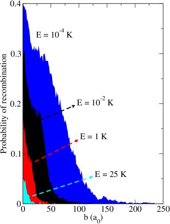
Figure 3: (Color online) Probability of recombination for helium atoms as a function of the impact parameter, at different collision energies: blue line, E = 10^-4 K; black line, E = 10^-2 K; red line, E = 1 K; cyan line, E = 25 K.

The TBRR for helium atoms as a function of the collision energy is presented in Fig. 4. The classical calculations have been performed following the methodology developed in Sec. III.3. Batches of 10⁵ trajectories have been computed for each collision energy, except for $E\geq 100$ K, for those energies 10⁶ trajectories are computed in order to have a reliable statistics in the three-body recombination events. The partial three-body rate for total angular momentum $J=0$ is also displayed. It is calculated by counting only those recombination trajectories having total angular momentum between $J=0$ and $J=\hbar$ and then applying Eqs. (27) and (28). The quantum mechanical calculation for $J^{\Pi}$ = $0^{+}$ has been carried out by means of the adiabatic hyperspherical representation outlined in Sec. IV. The quantum calculation has been divided by the symmetrization factor $3!$ in order to compare with the classical partial three-body rate; the $3!$ is a factor associated with the quantal indistinguishability of the colliding particles, and it is divided out to compare with the classical theory which of course treats the three particles as inherently distinguishable. This figure also shows the results of the three-body recombination rate coefficient for helium atoms deduced in a theoretical model based on the a simulation of the experimental conditions.Bruch et al. (2002) This model has some inputs that correspond with experimental values, whereas it has free parameters that are model dependent. The present calculations fix the scattering length of the helium dimer interaction, $a=172$ a₀Suno et al. (2002) and $\phi_{b}$=47 (see Ref. Bruch et al. (2002) for details of their model).

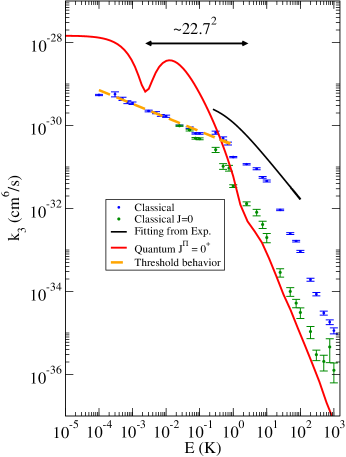
Figure 4: (Color online) The three-body recombination rate of helium atoms (in cm${}^{6}/$s) computed using different methods is shown as a function of the collision energy $E$ (in K). Solid red line: quantum calculation for a fixed total angular momentum and parity $J^{\Pi}$=0⁺. This calculations show convergence to within better than about 15$\%$ for $E$=1000 K. Blue points: classical trajectory calculations. Dark green points: classical trajectory calculations for a fixed total angular momentum $J$=0. Solid black line: theoretical model of Ref. Bruch et al. (2002).

Compare first the classical partial three-body rate for $J$ = 0 with the quantum calculation for the same total angular momentum. These calculations show good agreement for collision energies $E\gtrsim 1K$. The van der Waals energy $E_{\rm{vdW}}=\left(2\hbar^{6}/\mu^{3}C_{6}\right)^{1/2}$ is defined as a threshold energy between the ultracold physics $E$ ¡ $E_{vdW}$ and the thermal physics $E>E_{\rm{vdW}}$.Jones et al. (2006) For the helium dimer potential used in our calculations the van der Waals energy is $E_{\rm{vdW}}$ = 1.68 K, which marks the lowest energy where quantum and classical calculations begin to show the same trend, even though they are not yet in quantitative agreement at that energy.

Naturally the classical calculation exhibits no sign of the quantal interference minimum that is prominent around 2-4 mK. This quantal minimum is a universal feature associated with Efimov physics, as has been discussed previously.Suno et al. (2002); Shepard (2007); Rittenhouse et al. (2011) Esry and coworkers have stressed that the log-periodic behavior of Efimov physics, which originates in the attractive $1/r^{2}$ effective potential, should be observable in energy-dependences in addition to the more usual abscissa in ultracold experiments which is the scattering length. The small inflection in the quantal calculation around 20 K in Fig.4 is presumably the expected second interference feature, since it is seen close to where it is expected to appear, namely at an energy $22.7^{2}=515$ times the energy of the first interference minimum.Wang et al. (2013)

The classical calculations for three-body recombination rate (blue circles) show fair qualitative agreement with the three-body recombination rate coefficient (solid black line) obtained in the model of Bruch et al..Bruch et al. (2002) It is particulary interesting that the predictions of the model as well as the classical calculations show a change in the trend of the curves at around the same energy collision energy. We emphasize that the classical calculations are energy dependent, i.e. no Maxwell-Boltzmann thermal averaging has been performed, whereas the model of Bruch et al. is based on a thermally averaged recombination rate coefficient.

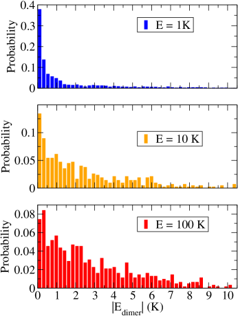
Figure 5: (Color online) Energy distribution of the helium dimers formed through three-body recombination trajectories at different collision energies: $E$ = 1 K, blue bars; $E$ = 10 K, orange bars; $E$ = 100 K, red bars.

Next, consider the behavior of the classical TBRR as a function of the collision energy for low energies $E\lesssim 1$ K. The trend of the classical calculations is well described by the orange dashed line. This line is a fit of the classical calculations to the classical ultracold threshold law for TBRR [Eq. (32)] derived above in the $n$-dimensional scattering method of Sec. III.4. As an independent test not related to our present calculation for helium, we have performed calculations for the TBRR as a function of the collision energy using a Lennard-Jones interaction between the atoms, and this test again agrees with the classical low energy threshold law. This numerical demonstration of the classical low energy threshold law confirms that the long-range interaction controls the low energy limit of classical three-body recombination.

The classical three-body rate behaves differently at $E\gtrsim 10$ K than it does at low collision energies. For collision energies higher than the the well depth, the classical trajectories are mainly deflected by the short-range part of the interaction, i.e. the hard inner wall of the two-body interaction starts to play a role. The helium dimer potential employed in our calculations has a well depth $\approx$11 K, which could explain the change in the trend of the classical calculation observed at that energy in Fig. 4.

In this vein, consider the energy distribution of the dimers formed in three-body recombination of helium atoms. This is presented in Fig. 5 as histogram of the dimer energies resulting from the three-body collisions. The distribution of dimer energies is observed to vary as one increases the collision energy. The energy distribution goes from a sharp distribution ($E$ = 1 K) to a flatter one ($E$ = 100 K). It is related to the role of the two-body interaction: for long-range dominated collisions the recombination processes start to occur at long distances between the atoms, leading mainly to the formation of shallow dimers. However, as one increases the collision energy, the recombination process will occur in inner regions of the atom-atom interaction, leading to an increasing of the probability to form dimers with higher binding energy.

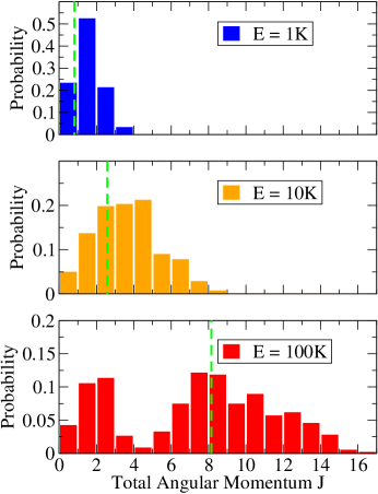
Figure 6: (Color online) Total angular momentum $J$ distribution associated with the recombination trajectories at three collision energies: $E$ = 1 K, blue bars; $E$ = 10 K, orange bars; $E$ = 100 K, red bars.

The distribution of total angular momentum $J$ of the classical recombination trajectories for different collision energies is plotted as a histogram in Fig. 6. This figure also plots the total angular momentum associated with the van der Waals length $R_{\rm{vdw}}=1/2\left(2\mu C_{6}/\hbar^{2}\right)^{1/4}$, which suggests a maximum value of the total angular momentum of the system contributing to recombination collisions if they are entirely dominated by the long-range interaction. It may be estimated as $J_{\rm{vdW}}\sim kR_{\rm{vdW}}$, where $R_{\rm{vdW}}$ is the van der Waals length and $k$ is the hyperspherical wave number. For the helium dimer interaction employed in this work it is $R_{\rm{vdW}}\approx$ 5 a₀. The results show good agreement between the most probable total angular momentum of the recombination trajectories and $J_{\rm{vdW}}$, except for the distribution at $E$ = 100 K, which shows a bimodal distribution. This bimodal distribution is presumably correlated with the change in the dimer energy distribution. For higher collision energies the probability to form dimers with high binding energy (small size) increases (see Fig. 5), so the contribution of small dimers will show up as a peak in the low total angular momentum. Indeed, this was noted in our discussion of Fig. 6. Finally, the change of trend in the classical three-body rate at $E\gtrsim 10$ K is evidently due to the increasing importance of the short-range interaction beyond that energy range. Moreover, the hard inner wall is responsible for the energy distribution of the dimers at high collision energies, and presumably for the bimodal distribution that deviates from the van der Waals estimation $J_{\rm{vdW}}$.

VI Summary

The present investigation has developed a general method to study classical scattering in $n$-dimensions. Application of this method to three-body collisions has shown a number of useful and interesting results: the classical ultracold threshold law for TBRR as a function of the collision energy and a high energy relationship between the classical three-body elastic cross section an the quantum one. The former has been shown numerically, the latter show a similar relationship that the two-body collision, leading to generalize the shadow scattering phenomena to three-body collisions.

The TBRR as a function of the collision energy for helium atoms has been calculated by the $n$-dimensional scattering method using classical trajectories. The general trends of the classical TBRR have been established the different influences of the long- versus short-range portions of the two-body interaction, as the collision energy changes. The classical results have been tested against our quantum mechanical TBRR, and the classical calculations accurately reproduce the trend of the quantum mechanical calculations for $E\gtrsim 1$ K. Nevertheless, quantitative agreement of the rates is not achieved, as a residual discrepancy between the high energy limits of classical and quantum TBRR is seen to be approximately.

Although the classical results have not quantitatively replicated the quantum mechanical results, especially at very low energies, the Newtonian treatment is a useful tool that can help in understanding three-body collisions. For instance, classical trajectory calculations provide a first estimate of the number of partial waves needed for a quantum mechanical calculation in the thermal regime. Also, use of classical trajectory methods to determine the energy distribution of the dimers formed allows an estimation of which dimer levels are the most important for quantum calculations. Finally, the interpretation of the TBRR through classical trajectory calculations gives important clues that can give insight into mechanisms relevant for the quantum mechanical calculations.

VII Acknowledgements

We are indebted to Jose D’Incao for his assistance and advice regarding the calculations. This work is supported in part by the U.S. Department of Energy, Office of Science.

References

- Brown et al. (1994) S. S. Brown, R. K. Taulkdar, and A. R. Ravishankara, Chem. Phys. Lett. 299, 277 (1994).
- Huang et al. (2012) H. Huang, A. J. Eskola, and C. A. Taatjes, J. Phys. Chem. Lett. 3, 3399 (2012).
- Schneider et al. (1995) L. Schneider, D. Seekamp-Rahn, J. Borkowski, E. Wrede, K. H. Welge, F. J. Aoiz, L. Bañares, M. J. D´Mello, V. J. Herrero, V. Sáez Rábanos, et al., Science 269, 207 (1995).
- Aoiz et al. (1998) F. J. Aoiz, L. Bañares, and V. J. Herrero, J. Chem. Soc. Faraday Trans. 94, 2483 (1998).
- Aoiz et al. (2005) F. J. Aoiz, V. Sáez-Rábanos, B. Martínez-Haya, and T. González-Lezana, J. Chem. Phys. 123, 094101 (2005).
- Jambrina et al. (2011) P. G. Jambrina, E. García, V. J. Herrero, V. Sáez-Rábanos, and F. J. Aoiz, J. Chem. Phys. 135, 034310 (2011).
- Homayoon et al. (2012) Z. Homayoon, P. G. Jambrina, F. J. Aoiz, and J. M. Bowman, J. Chem. Phys. 137, 021102 (2012).
- Li and Heller (2012) Z. Li and E. J. Heller, J. Chem. Phys. 136, 054306 (2012).
- Roberts et al. (1969) R. E. Roberts, R. B. Bernstein, and C. F. Curtiss, J. Chem. Phys. 50, 5163 (1969).
- Orel (1987) A. E. Orel, J. Chem. Phys. 87, 314 (1987).
- Wei et al. (1997) G. W. Wei, S. Alavi, and R. F. Snider, J. Chem. Phys. 106, 1463 (1997).
- Pack et al. (1998a) R. T. Pack, R. B. Walker, and B. K. Kendrick, J. Chem. Phys. 109, 6701 (1998a).
- Esposito and Capitelli (2009) F. Esposito and M. Capitelli, J. Phys. Chem. A 113, 15307 (2009).
- Colavecchia et al. (2003) F. D. Colavecchia, F. Mrugala, G. A. Parker, and R. T. Pack, J. Chem. Phys. 118, 10387 (2003).
- Forrey (2013) R. C. Forrey, Astrophys. J. Lett. 773, L25 (2013).
- (16) R. C. Forrey, arXiv:1307.0549.
- Ivanov and Babikov (2012) M. V. Ivanov and D. Babikov, J. Chem. Phys. 136, 184304 (2012).
- Azriel et al. (2011) V. M. Azriel, E. V. Kolesnikova, L. Yu Rusin, and M. B. Sevryuk, J. Phys. Chem. A 115, 7055 (2011).
- Charlo and Clary (2004) D. Charlo and D. Clary, J. Chem. Phys. 120, 2700 (2004).
- Xie et al. (2003) J. Xie, B. Poirier, and G. I. Gellene, J. Chem. Phys. 119, 10678 (2003).
- Bernshtein and Oref (2003) V. Bernshtein and I. Oref, J. Chem. Phys. 118, 10611 (2003).
- Karachevtsev and Vinogradov (1999) G. V. Karachevtsev and P. S. Vinogradov, Russian Rev. Chem. 68, 549 (1999).
- Parker et al. (2002) G. A. Parker, R. B. Walker, B. K. Kendrick, and R. T. Pack, J. Chem. Phys. 117, 6083 (2002).
- Pack et al. (1998b) R. T. Pack, R. B. Walker, and B. K. Kendrick, J. Chem. Phys. 109, 6714 (1998b).
- Smith (1962) F. T. Smith, Discuss. Faraday Soc. 33, 183 (1962).
- Lin (1995) C. D. Lin, Phys. Pep. 257, 1 (1995).
- Esry et al. (1996) B. D. Esry, C. D. Lin, and C. H. Greene, Phys. Rev. A 54, 394 (1996).
- Aymar et al. (1996) M. Aymar, C. H. Greene, and E. Luc-Koenig, Rev. Mod. Phys. 68, 1015 (1996).
- Tolstikhin et al. (1996) O. I. Tolstikhin, S. Watanabe, and M. Matsuzawa, J. Phys. B 29, L389 (1996).
- Wang et al. (2011) J. Wang, J. P. D´Incao, and C. H. Greene, Phys. Rev. A 84, 052721 (2011).
- Child (1974) M. S. Child, Molecular Collision Theory (Academic Press, London, England, 1974).
- Levine (2005) R. D. Levine, Molecular Reaction Dynamics (Cambridge University Press, Cambridge, England, 2005).
- Avery (1989) J. Avery, Hyperspherical Harmonics: Applications in Quantum Theory (Kluwer, Norwell, MA, 1989).
- Whittaker (1937) E. T. Whittaker, A Trataise on the Analytical Dynamics of Particles and Rigid Bodies (Cambridge University Press, Cambridge, England, 1937).
- Karplus et al. (1965) M. Karplus, R. N. Porter, and R. D. Sharma, J. Chem. Phys. 43, 3259 (1965).
- Aziz et al. (1995) R. A. Aziz, A. R. Janzen, and M. R. Moldover, Phys. Rev. Lett 74, 1586 (1995).
- Press et al. (1986) W. H. Press, S. A. Teukolsky, W. T. Vetterling, and B. P. Falnnery, Numerical Recipes in Fotran 77 (Cambridge University Press, Cambridge, England, 1986).
- Esry et al. (1999) B. D. Esry, C. H. Greene, and J. P. Burke Jr., Phys. Rev. Lett 83, 1751 (1999).
- Suno et al. (2002) H. Suno, B. D. Esry, C. H. Grene, and J. P. Burke Jr., Phys. Rev. A 65, 042725 (2002).
- Wang et al. (2012) J. Wang, J. P. D´Incao, Y. Wang, and C. H. Greene, Phys. Rev. A 86, 062511 (2012).
- Yu. Schreiber (1966) A. Yu. Schreiber, ed., The Monte Carlo Method: The Method for Statistical Trials (Pergamon Press, Oxford, 1966).
- Landau and Binder (2009) D. P. Landau and K. Binder, A guide to Monte-Carlo Simulations in Statistical Physics (Cambridge University Press, Cambridge, England, 2009).
- Truhlar and Muckerman (1975) D. G. Truhlar and J. T. Muckerman, in Atom-Molecule Collision Theory: A Guide for the Experimentalist, edited by R. B. Bernstein (Plenum Press, New York, 1975), chap. 16, pp. 505–566.
- Shui (1972) V. H. Shui, Ph.D. thesis, Deparment of mechanical ingeneering MIT (1972).
- Shui (1973) V. H. Shui, J. Chem. Phys. 58, 4868 (1973).
- Landau and Lifshitz (1958) L. D. Landau and E. M. Lifshitz, Quantum Mechanics (Butterworht Heinemann, Oxfort, England, 1958).
- Kendrick et al. (1999) B. K. Kendrick, R. T. Pack, R. B. Walker, and E. F. Hayes, J. Chem. Phys. 110, 6673 (1999).
- Lepetit et al. (1990) B. Lepetit, Z. Peng, and A. Kuppermann, Chem. Phys. Lett. 166, 572 (1990).
- Suno and Esry (2008) H. Suno and B. D. Esry, Phys. Rev. A 78, 062701 (2008).
- Mott and Massey (1965) N. F. Mott and H. S. W. Massey, The Theory of Atomic Collisions (Claredon Press, Oxford, 1965), 3rd ed.
- Mehta et al. (2009) N. P. Mehta, S. T. Rittenhouse, J. P. D´Incao, J. von Stecher, and C. H. Greene, Phys. Rev. Lett 103, 153201 (2009).
- Bruch et al. (2002) L. W. Bruch, W. Schöllkopf, and J. P. Toennies, J. Chem. Phys. 117, 1544 (2002).
- Jones et al. (2006) K. M. Jones, E. Tiesinga, P. D. Lett, and P. S. Julienne, Rev. Mod. Phys. 78, 483 (2006).
- Shepard (2007) J. R. Shepard, Phys. Rev. A 75, 062713 (2007).
- Rittenhouse et al. (2011) S. T. Rittenhouse, J. von Stecher, J. P. D´Incao, N. P. Mehta, and C. H. Greene, J. Phys. B 44, 172001 (2011).
- Wang et al. (2013) Y. Wang, J. P. D´Incao, and B. D. Esry, Adv. At. Mol. Phys. 62, 1 (2013).