Including realistic tidal deformations in binary black-hole initial data

Abstract

A shortcoming of current binary black-hole initial data is the generation of spurious gravitational radiation, so-called junk radiation, when they are evolved. This problem is a consequence of an oversimplified modeling of the binary’s physics in the initial data. Since junk radiation is not astrophysically realistic, it contaminates the actual waveforms of interest and poses a numerical nuisance. The work here presents a further step towards mitigating and understanding the origin of this issue, by incorporating post-Newtonian results in the construction of constraint-satisfying binary black-hole initial data. Here we focus on including realistic tidal deformations of the black holes in the initial data, by building on the method of superposing suitably chosen black hole metrics to compute the conformal data. We describe the details of our initial data for an equal-mass and nonspinning binary, compute the subsequent relaxation of horizon quantities in evolutions, and quantify the amount of junk radiation that is generated. These results are contrasted with those obtained with the most common choice of conformally flat (CF) initial data, as well as superposed Kerr-Schild (SKS) initial data. We find that when realistic tidal deformations are included, the early transients in the horizon geometries are significantly reduced, along with smaller deviations in the relaxed black hole masses and spins from their starting values. Likewise, the junk radiation content in the $l=2$ modes is reduced by a factor of $\sim$1.7 relative to CF initial data, but only by a factor of $\sim$1.2 relative to SKS initial data. More prominently, the junk radiation content in the $3\leq l\leq 8$ modes is reduced by a factor of $\sim$5 relative to CF initial data, and by a factor of $\sim$2.4 relative to SKS initial data.

I Introduction

A key objective of numerical relativity is to accurately model the inspiral and coalescence of black-hole binaries, which are important sources of gravitational waves that are expected to be observed by detectors such as LIGO et al. (2006) and VIRGO di Fiore (2002) in the near future. Any simulation of a black-hole binary must begin with the construction of suitable initial data, which are a solution to the Einstein constraint equations, that ideally capture as many relevant features of the physical system as possible. Presently though, the majority of initial data assumes that the spatial metric is conformally flat, a choice dictated by convenience. It is known that conformal flatness is generally incompatible with desired black hole solutions. For instance, a Kerr black hole with nonzero spin does not admit a conformally flat slicing Garat and Price (2000); Valiente Kroon (2004), and neither does a black-hole binary starting at ${\mathcal{O}\left(v^{4}\right)}$ in the post-Newtonian (PN) approximation Nissanke (2006), where $v$ is the binary’s orbital velocity, in units of the speed of light $c$.

One side effect of conformally flat initial data for black-hole binaries is the generation of spurious gravitational radiation, so-called junk radiation, when they are evolved. Junk radiation contaminates the waveforms of interest, and interferes with their comparison to PN predictions Boyle et al. (2007); Hannam et al. (2008). Computational resources are also wasted in waiting for the junk radiation to propagate off the computational domain, before reliable waveforms can be extracted. Resolving the high-frequency components of the junk radiation requires a large increase in numerical resolution as well Zlochower et al. (2012), which slows down the evolution appreciably. The initial properties of the black holes themselves are also altered by the junk radiation, relaxing to slightly different values later on in the evolution. Additionally, junk radiation disturbs the orbital trajectories and complicates the construction of initial data with low eccentricity, which applies to binaries formed from stellar evolution Postnov and Yungelson (2005). Recently though, an iterative scheme was demonstrated to be effective at jointly reducing eccentricity and junk radiation Zhang and Szilágyi (2013).

Over the last several years, various efforts have been made to go beyond the assumption of conformal flatness, by using conformally curved initial data. A direct superposition of black hole metrics was introduced in Matzner et al. (1998); Marronetti and Matzner (2000); Marronetti et al. (2000) to specify the conformal metric, and a similar procedure was shown in Hannam et al. (2007) to reduce the junk radiation in the head-on collision of two black holes. Later on, a weighted superposition of black hole metrics was used in Lovelace et al. (2008); Lovelace (2009), and decreased the amount of junk radiation in the inspiral of two equal-mass, nonspinning black holes Lovelace (2009). These superposed black-hole initial data already provide a notable improvement over conformally flat initial data, but they do not take advantage of all the available information to better represent the binary’s physics, such as results from PN theory Blanchet (2006). Including such information could prove to be very useful.

Initial data incorporating the PN approximation include that of Nissanke (2006), which has interaction terms between the black holes in the conformal metric, and that of Kelly et al. (2007), which contains the outgoing gravitational radiation of the binary in the conformal metric. The initial data in Kelly et al. (2007) was evolved in Kelly et al. (2010); Mundim et al. (2011), and was found to reduce the low-frequency components of the junk radiation. However, currently such initial data are largely restricted to nonspinning black holes. Furthermore, the regions near the black holes are not adequately treated in the approaches above, because no attempt was made to account for the tidal deformations.

The aforementioned issue was addressed in Johnson-McDaniel et al. (2009), by describing the vicinity of the black holes by tidally perturbed Schwarzschild metrics in horizon penetrating coordinates, which were asymptotically matched to a PN metric to determine the tidal fields. This procedure has now been extended to spinning black holes Gallouin et al. (2012). These studies follow the earlier work of Yunes et al. (2006); Yunes and Tichy (2006), which used black hole metrics in coordinates that were not horizon penetrating from the outset, and were thus inconvenient for numerical implementation. Including tidal deformations is expected to reduce the high-frequency components of the junk radiation, which are typically attributed to physically unrealistic deformations of the black holes in the initial data that radiate away as the black hole geometries relax in an evolution. The initial data of Johnson-McDaniel et al. (2009) was adapted to moving punctures and evolved in Reifenberger and Tichy (2012). However, only the lower-frequency $\left(2,2\right)$ mode of the junk radiation was studied. We also point out that all the previous initial data sets using PN corrections only approximately satisfied the Einstein constraint equations, and were not used to provide free data for a constraint solver. This had adverse manifestations in an evolution, such as the black holes losing mass.

The present work examines the effects of including realistic tidal deformations in the context of superposed black-hole initial data, both elucidating the origin and quantifying the amount of junk radiation that is associated with modeling the horizon geometries. It also represents a first step in using PN results to construct constraint-satisfying initial data that future efforts can build on. In particular, we construct excision initial data for an equal-mass, nonspinning black-hole binary in the extended conformal-thin-sandwich formalism using a similar method as in Lovelace et al. (2008); Lovelace (2009), by superposing two tidally perturbed Schwarzschild metrics given in Johnson-McDaniel et al. (2009). The Einstein constraint equations are solved with the pseudospectral elliptic solver of Pfeiffer et al. (2003), and the initial data are evolved for the early inspiral phase following the techniques found in Szilagyi et al. (2009). These results are then contrasted with those for conformally flat initial data and superposed Kerr-Schild initial data, which both do not have realistic tidal deformations.

This paper is organized as follows. Section II summarizes the extended-conformal-thin-sandwich formalism for constructing initial data, and details our choices for the freely specifiable data and boundary conditions. Section III presents the evolutions of our initial data, and inspects various properties of the black hole horizons at early times. The junk radiation content that is generated in the evolutions is also quantified. Section IV gives final remarks on our results and discusses potential directions for future work.

II Initial Data

II.1 Extended-conformal-thin-sandwich equations

Initial data is constructed within the extended-conformal-thin-sandwich formalism York (1999); Pfeiffer and York (2003). First, the spacetime metric is decomposed into $3+1$ form Arnowitt et al. (1962); York, Jr. (1979)

$$^{(4)}ds^{2} =g_{\mu\nu}dx^{\mu}dx^{\nu},$$ (1)

$$=-N^{2}dt^{2}+g_{ij}\left(dx^{i}+\beta^{i}dt\right)\left(dx^{j}+\beta^{j}dt\right),$$ (2)

where $g_{ij}$ is the spatial metric of a $t=\text{constant}$ hypersurface $\Sigma_{t}$, $N$ is the lapse function, and $\beta^{i}$ is the shift vector. (Here and throughout this paper, Greek indices are spacetime indices running from 0 to 3, while Latin indices are spatial indices running from 1 to 3.) The Einstein equations then become a set of evolution equations,

$$(\partial_{t}-\mathcal{L}_{\beta})g_{ij} =-2NK_{ij},$$ (3)

$$(\partial_{t}-\mathcal{L}_{\beta})K_{ij} =N\left(R_{ij}-2K_{ik}{K^{k}}_{j}+KK_{ij}\right)-\nabla_{i}\nabla_{j}N,$$ (4)

and a set of constraint equations,

$$R+K^{2}-K_{ij}K^{ij} =0,$$ (5)

$$\nabla_{j}\left(K^{ij}-g^{ij}K\right) =0.$$ (6)

Equation (5) is known as the Hamiltonian constraint, and Eq. (6) is the momentum constraint. In the above, all matter source terms have been neglected, since we will only be interested in vacuum spacetimes. Also, $\mathcal{L}$ is the Lie derivative, $\nabla_{i}$ is the covariant derivative compatible with $g_{ij}$, $R=g^{ij}R_{ij}$ is the trace of the Ricci tensor $R_{ij}$ of $g_{ij}$, and $K=g^{ij}K_{ij}$ is the trace of the extrinsic curvature $K_{ij}$ of $\Sigma_{t}$.

Initial data	$\bm{M_{\rm ADM}/M}$	$\bm{J_{\rm ADM}/M^{2}}$	$\bm{d_{0}/M}$	$\bm{s_{0}/M}$	$\bm{M\Omega_{0}}$	$\bm{\dot{r}_{0}/r_{0}}$	$\bm{e}$	$\bm{\chi_{0}}$
CFMS	0.992402	1.0898	14.44	17.37	0.0167081	$-2.84\times 10^{-5}$	$5\times 10^{-5}$	$2.05574\times 10^{-7}$
SKS	0.992629	1.1046	15.0	16.90	0.0158313	$-4.79\times 10^{-5}$	$2\times 10^{-4}$	$1.05715\times 10^{-7}$
STPv1	0.992699	1.1223	15.0	17.68	0.0156354	0.0	$1\times 10^{-2}$	$4.33909\times 10^{-6}$
STPv2	0.992539	1.1093	15.0	17.68	0.0156354	0.0	$1\times 10^{-2}$	$3.51594\times 10^{-5}$

Table 1: Summary of our initial data properties, where $M_{\text{ADM}}$ is the Arnowitt-Deser-Misner (ADM) energy, $J_{\text{ADM}}$ is the ADM angular momentum, $d_{0}$ is the initial coordinate separation, $s_{0}$ is the initial proper separation, $\Omega_{0}$ is the initial orbital frequency, $\dot{r_{0}}/r_{0}$ is the initial radial velocity of one black hole, $e$ is the eccentricity, and $\chi_{0}$ is the initial dimensionless spin magnitude of one black hole.

The spatial metric is decomposed in terms of a conformal metric ${\tilde{g}}_{ij}$ and a conformal factor $\psi$,

$$g_{ij}=\psi^{4}{\tilde{g}}_{ij}.$$ (7)

The tracefree time derivative of the conformal metric is denoted by

$$\tilde{u}_{ij}=\partial_{t}{\tilde{g}}_{ij},$$ (8)

and satisfies $\tilde{u}_{ij}\tilde{g}^{ij}=0$. A conformal lapse is also defined by $\tilde{N}=\psi^{-6}N$. Treating $N\psi=\tilde{N}\psi^{7}$ as an independent variable, Eqs. (5), (6), and the trace of (4) can then be written as

$$\tilde{\nabla^{2}}\psi-\frac{1}{8}\psi\tilde{R}-\frac{1}{12}\psi^{5}K^{2}+\frac{1}{8}\psi^{-7}\tilde{A}_{ij}\tilde{A}^{ij}=0,$$ (9)

$$\tilde{\nabla}_{j}\left(\frac{\psi^{7}}{2\left(N\psi\right)}\left(\mathbb{L}\beta\right)^{ij}\right)-\tilde{\nabla}_{j}\left(\frac{\psi^{7}}{2\left(N\psi\right)}\tilde{u}^{ij}\right)-\frac{2}{3}\psi^{6}\tilde{\nabla}^{i}K=0,$$ (10)

$$\tilde{\nabla}^{2}\left(N\psi\right)-\left(N\psi\right)\left(\frac{1}{8}\tilde{R}+\frac{5}{12}\psi^{4}K^{2}+\frac{7}{8}\psi^{-8}\tilde{A}_{ij}\tilde{A}^{ij}\right)$$

$$=-\psi^{5}\left(\partial_{t}K-\beta^{k}\partial_{k}K\right).$$ (11)

In the above, $\tilde{\nabla}_{i}$ is the covariant derivative compatible with $\tilde{g}_{ij}$, $\tilde{R}=\tilde{g}^{ij}\tilde{R}_{ij}$ is the trace of the Ricci tensor $\tilde{R}_{ij}$ of $\tilde{g}_{ij}$, $\tilde{\mathbb{L}}$ is the longitudinal operator,

$$\left(\tilde{\mathbb{L}}\beta\right)^{ij}=\tilde{\nabla}^{i}\beta^{j}+\tilde{\nabla}^{j}\beta^{i}-\frac{2}{3}\tilde{g}^{ij}\tilde{\nabla}_{k}\beta^{k},$$ (12)

and $\tilde{A}^{ij}$ is

$$\tilde{A}^{ij}=\frac{1}{2\tilde{N}}\left(\left(\tilde{\mathbb{L}}\beta\right)^{ij}-\tilde{u}^{ij}\right),$$ (13)

which is related to $K_{ij}$ by

$$K_{ij}=\psi^{-10}\tilde{A}_{ij}+\frac{1}{3}g_{ij}K.$$ (14)

Given a particular choice for the freely specifiable data

$$\left(\tilde{g}_{ij},\tilde{u}_{ij},K,\partial_{t}K\right),$$ (15)

Eqs. (9), (10), and (II.1) constitute a coupled set of elliptic equations that one solves for $\psi$, $N\psi$, and $\beta^{i}$. These equations are known as the extended-conformal-thin-sandwich equations. From their solutions, the physical initial data $g_{ij}$ and $K_{ij}$ are obtained from Eqs. (7) and (14), respectively.

Figure 1: Convergence of the $L^{2}$ norms of the Hamiltonian and momentum constraints for different types of initial data, with increasing number of grid points $N$ in the computational domain.

II.2 Types of initial data

Our initial data represent two equal-mass, nonspinning black holes, each with an initial Christodoulou mass $m=M/2$, which are situated $\sim$16 orbits before merger. Equations  (9), (10), and (II.1) are solved with the pseudospectral elliptic solver detailed in Pfeiffer et al. (2003). The singularities of the black holes are excised from the computational domain. The initial data sets described below differ in their choices for the freely specifiable $\tilde{g}_{ij}$ and $K$, and the boundary conditions imposed at the excision surfaces $\mathcal{S}$. In all cases, we set the freely specifiable time derivatives to zero in the corotating frame of the binary,

$$\tilde{u}_{ij}=0,\hskip 5.69054pt\partial_{t}K=0.$$ (16)

In terms of a radial coordinate $r$ measured from the center of mass, the outer boundary is placed at a large distance $R_{\text{large}}/M=1.0\times 10^{9}$, where asymptotic flatness is imposed in the inertial frame of the binary,

$$\left.\psi\right|_{R_{\text{large}}} =N\psi|_{R_{\text{large}}}=1,$$ (17)

$$\left.\beta^{i}\right|_{R_{\text{large}}} =0.$$ (18)

II.2.1 Conformally flat, maximally sliced initial data

Conformal flatness is currently the most common choice in constructing black hole initial data, especially in the Bowen-York formulation Bowen and York, Jr. (1980) for codes that use puncture methods, because the constraint equations, Eqs. (5)–(6), simplify greatly. For our purposes, we consider conformally flat and maximally sliced (CFMS) initial data, identical to that used in Boyle et al. (2007); M. Scheel, M. Boyle, T. Chu, L. Kidder, K. Matthews and H. Pfeiffer (2009). That is, the remaining free data are fixed by a flat conformal metric,

$$\tilde{g}_{ij}=\delta_{ij},$$ (19)

along with the maximal slicing condition Lichnerowicz (1944); Smarr and York (1978),

$$K=0.$$ (20)

Quasi-equilibrium boundary conditions Cook and Pfeiffer (2004) for $\psi$ and $\beta^{i}$ are imposed on spherical excision surfaces, with $\left.\beta^{i}\right|_{\mathcal{S}}$ adjusted so that the spins $\chi$ Lovelace et al. (2008) of the black holes are very small. The lapse boundary condition is given by Caudill et al. (2006)

$$\frac{d\left(N\psi\right)}{dr}\bigg{|}_{\mathcal{S}}=0.$$ (21)

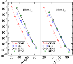
The initial orbital eccentricity was reduced to $e\sim 5\times 10^{-5}$ using the iterative procedure in Pfeiffer et al. (2007), giving an initial orbital frequency $M\Omega_{0}=0.0167081$ and radial velocities $\dot{r}_{0}/r_{0}=-2.84\times 10^{-5}$. Properties of CFMS initial data are summarized in Table 1. The convergence of the Hamiltonian and momentum constraints are shown in Fig. 1, as the red triangles connected by the dotted lines. Plotted is the $L^{2}$ normof the Hamiltonian constraint and the root-sum-square of the $L^{2}$ norms of the momentum constraint components, versus the total number of grid points $N$ in the initial data domain. Due to the simple structure of the conformal data, less grid points are needed to resolve the solution in contrast to the other types of conformally curved initial data we present below.

II.2.2 Superposed Kerr-Schild initial data

Another type of initial data in use is based on the superposition of black hole metrics, as first presented in Matzner et al. (1998); Marronetti and Matzner (2000); Marronetti et al. (2000). Here we follow the variant of Lovelace et al. Lovelace et al. (2008) in constructing superposed Kerr-Schild (SKS) initial data.  In this approach, the remaining free data are taken to be a weighted superposition of the corresponding quantities for a boosted, nonspinning Kerr-Schild black hole,

$$\tilde{g}_{ij} =\delta_{ij}+\displaystyle\sum\limits_{a=1}^{2}e^{-r^{2}_{a}/w^{2}_{a}}\left(g^{a}_{ij}-\delta_{ij}\right),$$ (24)

$$K =\displaystyle\sum\limits_{a=1}^{2}e^{-r^{2}_{a}/w^{2}_{a}}K_{a},$$ (25)

where $g^{a}_{ij}$ and $K_{a}$ are the spatial metric and trace of the extrinsic curvature, respectively, of a Kerr-Schild black hole (labeled by $a$) with mass $\tilde{m}^{\text{KS}}_{a}$ and speed $\tilde{v}^{\text{KS}}_{a}$. The Gaussian factor $e^{-r^{2}_{a}/w^{2}_{a}}$, for a fixed weight parameter $w_{a}$, is a function of Euclidean distance $r_{a}$ from black hole $a$. Its presence ensures that in the vicinity of each black hole, the conformal data approach the appropriate Kerr-Schild values, while far away from the black holes the conformal data approach that of a flat spacetime.

Unlike CFMS initial data, the excision surfaces are not coordinate spheres, but are Lorentz-contracted along the direction of the boost. Quasi-equilibrium boundary conditions Cook and Pfeiffer (2004) for $\psi$ and $\beta^{i}$ are still imposed on $\mathcal{S}$, with the black hole spins $\chi$ made very small. However, the following Dirichlet boundary condition for the lapse is used,

$$\left.N\psi\right|_{\mathcal{S}}=1+\displaystyle\sum\limits_{a=1}^{2}e^{-r^{2}_{a}/w^{2}_{a}}\left(N_{a}-1\right),$$ (26)

where $N_{a}$ is the lapse of the corresponding Kerr-Schild black hole.

For the parameters entering our SKS initial data, we use $\tilde{m}^{\text{KS}}_{a}=0.37298$, $w_{a}/\tilde{m}^{\text{KS}}_{a}=6$, and $\tilde{v}^{\text{KS}}_{a}=0.11873$. The value of $\tilde{m}^{\text{KS}}_{a}$ was set so that $m=0.5$ and $M=1$. Also, the value of $w_{a}$ was chosen to approximately minimize the junk radiation content. The convergence of the Hamiltonian and momentum constraints are shown in Fig. 1, as the blue squares connected by the dashed lines.

The initial eccentricity was reduced to $e\sim 2\times 10^{-4}$ using the iterative procedure in Pfeiffer et al. (2007), giving an initial orbital frequency $M\Omega_{0}=0.0158313$ and radial velocities $\dot{r}_{0}/r_{0}=-4.79\times 10^{-5}$. Although the eccentricity could have been reduced further without difficulty, doing so was not important for our present purposes. Properties of SKS initial data are summarized in Table 1. The convergence of the Hamiltonian and momentum constraints are shown in Fig. 1, as the blue squares connected by the dashed lines.

II.2.3 Superposed tidally perturbed initial data

To include realistic tidal deformations of the black holes in our initial data, we build on the method presented above and construct superposed tidally perturbed (STP) initial data. Instead of Kerr-Schild metrics, which only characterize isolated black holes, we make use of suitable tidally perturbed black hole metrics that have been determined by Johnson-McDaniel et al. Johnson-McDaniel et al. (2009). Their metrics are obtained by asymptotically matching perturbed Schwarzschild metrics in horizon-penetrating Cook-Scheel harmonic coordinates Cook and Scheel (1997), to an order $\mathcal{O}\left(v^{4}\right)$ PN near zone metric Blanchet et al. (1998) in harmonic coordinates for two point particles in a circular orbit. To perform the matching, the black hole metrics are perturbatively transformed to the same coordinate system as the PN metric. The matching then determines this coordinate transformation up to $\mathcal{O}\left(v^{5}\right)$, as well as the Newtonian quadrupole and octupole tidal fields and the 1PN corrections to the quadrupole fields in the black hole metrics. In the appendix, we collect the explicit expressions for these quantities.

The fact that horizon-penetrating coordinates are used for the black hole metrics from the start is important for us, even though the PN harmonic coordinates themselves are not horizon-penetrating. This is because after perturbatively transforming to PN harmonic coordinates, the black hole metrics remain in horizon-penetrating coordinates, so that we can use excision in constructing initial data. Nevertheless, we only apply the transformation up to $\mathcal{O}\left(v^{3}\right)$, as the lowest-order piece between Cook-Scheel and PN harmonic coordinates for an unperturbed Schwarzschild black hole enters at $\mathcal{O}\left(v^{4}\right)$, and we find that the constraint violations (before solving the constraint equations) are larger when the higher-order pieces are included. This should not cause too much concern for our present purposes, since we are not yet including the PN near zone metric in our conformal data, so that placing the black hole metrics as closely as possible into PN harmonic coordinates is not crucial. Moreover, the lowest-order pieces of the Lorentz boost for the black holes’ orbital motion are already present at $\mathcal{O}\left(v^{3}\right)$, which is the highest order for which all pieces of the coordinate transformation are fixed by the matching.

The remaining free data for our STP initial data are then chosen as in Eqs. (24)–(25), but now $g^{a}_{ij}$ and $K_{a}$ are the spatial metric and trace of the extrinsic curvature, respectively, of a tidally perturbed black hole mentioned above. Thus, while the conformal data include realistic tidal deformations in the vicinity of each black hole, they still approach that of a flat spacetime between and far away from the black holes. That is, there are no PN interaction terms in the near zone surrounding the black holes, nor any outgoing radiation content in the wave zone.

We use spherical excision surfaces, and impose the following Dirichlet boundary conditions there,

$$\left.N\psi\right|_{\mathcal{S}} =1+\sum_{a=1}^{2}e^{-r_{a}^{2}/w_{a}^{2}}(N_{a}-1),$$ (27)

$$\left.\beta^{i}\right|_{\mathcal{S}} =\sum_{a=1}^{2}e^{-r_{a}^{2}/w_{a}^{2}}\beta_{a}^{i},$$ (28)

where $N_{a}$ and $\beta_{a}^{i}$ are the lapse and shift, respectively, of the corresponding tidally perturbed black hole. The boundary condition on $\beta^{i}$ also fixes the black hole spins $\chi_{0}$, which still have values close to zero (cf. Table 1). We do not use quasi-equilibrium boundary conditions Cook and Pfeiffer (2004) here, since they were derived by requiring an excision surface to be an apparent horizon on which the outgoing null normals have vanishing shear. For a tidally perturbed black hole however, the apparent horizon foliates a dynamical horizon Booth (2005) and has non-vanishing shear, so imposing quasi-equilibrium boundary conditions would not be appropriate.

There are several additional parameters that we need to choose in constructing our initial data. These are the mass parameter $\tilde{M}$ in Cook-Scheel coordinates of Eqs. (A)–(A), plus the mass parameters $\tilde{m}_{1}=\tilde{m}_{2}$ and separation parameter $b$ in PN harmonic coordinates that appear in Eqs. (44)–(54). Since $\tilde{M}$ and $\tilde{m}_{1}=\tilde{m}_{2}$ are found to be identical up to the highest order fixed by the asymptotic matching Johnson-McDaniel et al. (2009), we set them to equal to each other, $\tilde{M}=\tilde{m}_{1}=\tilde{m}_{2}=0.5036$. This value was chosen so that $m=0.5$ and $M=1$. The separation parameter is simply taken to be the coordinate distance between the two apparent horizons in our initial data, that is $b/M=d_{0}/M=15$. In addition, we set $w_{a}/\tilde{M}=13$ for the superposition to approximately minimize the junk radiation content.

We consider two versions of STP initial data. The first verion incorporates all the terms in the tidal fields (44)–(47), which we call STPv1. The second, STPv2, includes only the lowest-order piece of the tidal field, the Newtonian electric quadrupole, with a “corotating” time dependence obtained via the substitutions

$$\hat{x}_{i} \rightarrow\hat{x}_{i}\text{cos}\omega t+\hat{y}_{i}\text{sin}\omega t,$$ (29)

$$\hat{y}_{i} \rightarrow-\hat{x}_{i}\text{sin}\omega t+\hat{y}_{i}\text{cos}\omega t.$$ (30)

Having these versions allows us to investigate the importance of including the higher-order contributions of the tidal fields. This is especially relevant given that recently a lowest-order tidally perturbed metric with spin, with a corotating time dependence of the tidal fields, has become available Gallouin et al. (2012).

It should be noted that the parameters $\tilde{m}_{1}$, $\tilde{m}_{2}$, and $b$ used in transforming from Cook-Scheel to PN harmonic coordinates also affect the initial boost velocities of the black holes. The black holes would be on very nearly circular orbits, if the initial data were exactly in PN harmonic coordinates (and assuming the black holes are sufficiently far apart so that the PN approximation is valid). Due to the superposition procedure, our initial data are not in PN harmonic coordinates, and this gives rise to a rather large initial eccentricity of $e$$\sim$0.01. The eccentricity could possibly be reduced by adjusting the values of these parameters, and the weight parameters $w_{a}$ in the superposition, as the latter also influence the properties of the black holes. Another way is to include higher-order boost pieces in the coordinate transformation, with an adjustable free parameter Johnson-McDaniel (2012). For this paper though, we do not explore the results of these procedures.

Properties of our STP initial data are summarized in Table 1. The convergence of the Hamiltonian and momentum constraints are shown in Fig. 1. The values of the constraints are displayed as the black circles connected by solid lines for STPv1 initial data, and the unconnected green stars for STPv2 initial data.

III Evolutions

The initial data sets are evolved with similar methods as in Szilagyi et al. (2009). We use the Spectral Einstein Code (SpEC) Scheel et al. (2006); SpE to solve a first-order representation Lindblom et al. (2006) of the generalized harmonic system Friedrich (1985); Garfinkle (2002); Pretorius (2005), on a computational domain from which the singularities are excised. To accommodate the use of excision, two distinct coordinate frames are used: the “grid frame” that follows the motion of the black holes, and the “inertial frame” that is non-rotating and asymptotically Minkowski. The dynamical fields in the evolution equations are solved for in inertial-frame coordinates $x^{i}$, as functions of the grid-frame coordinates $\bar{x}^{i}$.

Figure 2: Constraint violations during the evolutions of different initial data. Plotted is the $L^{2}$ norm of all constraints, normalized by the $L^{2}$ norm of the spatial gradients of all dynamical fields.

In the computational domain, the excision boundaries are located just inside the apparent horizons, which differ marginally for the various types of initial data. The rest of the grid structures (consisting of touching spherical shells, cubes, and cylinders) remain the same. The outer boundaries are placed at $R_{\text{outer}}/M=480$. No boundary conditions are imposed at the excision surfaces, because all characteristic fields of the system are outgoing (into the black hole) there. The outer boundary conditions Lindblom et al. (2006); Rinne (2006); Rinne et al. (2007) imposed prevent the influx of unphysical constraint violations Stewart (1998); Friedrich and Nagy (1999); Bardeen and Buchman (2002); Szilágyi et al. (2002); Calabrese et al. (2003); Szilágyi and Winicour (2003); Kidder et al. (2005) and undesired incoming gravitational radiation Buchman and Sarbach (2006, 2007), while allowing the outgoing gravitational radiation to pass freely through. Interdomain boundary conditions are enforced with a penalty method Gottlieb and Hesthaven (2001); Hesthaven (2000).

The gauge freedom in the generalized harmonic system is fixed through a freely specifiable gauge source function $H_{\mu}$ given by

$$H_{\mu}(t,x)=g_{\mu\nu}\nabla_{\lambda}\nabla^{\lambda}x^{\nu}=-\Gamma_{\mu},$$ (31)

where $\Gamma_{\mu}=g^{\nu\lambda}\Gamma_{\mu\nu\lambda}$ is the trace of the Christoffel symbol. In $3+1$ form, this becomes a set of evolution equations for $N$ and $\beta^{i}$ Lindblom et al. (2008). During the early inspiral, which is the only phase of the evolution considered here, the gauge is fixed by the quasi-equilibrium condition

$$\partial_{\bar{t}}\tilde{H}_{\mu}=0,$$ (32)

where $\tilde{H}_{\mu}$ is a tensor defined such that $\tilde{H}_{\mu}=H_{\mu}$ in the inertial frame.

Figure 3: Extrema of the intrinsic scalar curvature $m^{2}\bar{R}$ over a black hole’s apparent horizon, in the evolution of different initial data sets.

      

Figure 4: Intrinsic scalar curvature $m^{2}\bar{R}$ of a black hole horizon in the evolution of CFMS initial data, minus the Schwarzschild value of 0.5. On the left are values at $t/M=0$. On the right are values at $t_{\text{relaxed}}/M=250$.

      

Figure 5: Intrinsic scalar curvature $m^{2}\bar{R}$ of a black hole horizon in the evolution of SKS initial data, minus the Schwarzschild value of 0.5. On the left are values at $t/M=0$. On the right are values at $t_{\text{relaxed}}/M=250$.

      

Figure 6: Intrinsic scalar curvature $m^{2}\bar{R}$ of a black hole horizon in the evolution of STPv1 initial data, minus the Schwarzschild value of 0.5. On the left are values at $t/M=0$. On the right are values at $t_{\text{relaxed}}/M=250$.

      

Figure 7: Intrinsic scalar curvature $m^{2}\bar{R}$ of a black hole horizon in the evolution of STPv2 initial data, minus the Schwarzschild value of 0.5. On the left are values at $t/M=0$. On the right are values at $t_{\text{relaxed}}/M=250$.

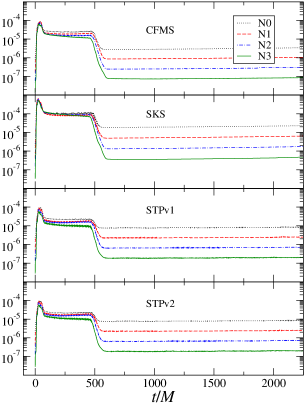
Each initial data set is evolved on four different resolutions, N0, N1, N2, and N3. These correspond to approximately $65^{3}$, $71^{3}$, $78^{3}$, and $85^{3}$ grid points, respectively. During the evolutions, neither the Hamiltonian and momentum constraints, nor the secondary constraints of the first-order generalized harmonic evolution system are explicitly enforced. By monitoring the constraint violations, we can obtain an indication of the accuracy of the evolutions. Their values are shown in Fig. 2. Plotted is the $L^{2}$ norm of all the constraint fields of the first-order generalized harmonic system, normalized by the $L^{2}$ norm of the spatial gradients of the dynamical fields (cf. Eq. (71) in Lindblom et al. (2006)). The $L^{2}$ norms are taken over the portion of the computational volume that lies outside the apparent horizons. Below, we present the results from our evolutions with the highest resolution N3.

III.1 Horizon properties

One would like to capture the correct horizon geometries as much as possible in the initial data, in order to avoid transients at early times as the black holes relax. We can visualize the deformations that a black hole undergoes by plotting the intrinsic scalar curvature $\bar{R}$ of its apparent horizon at various times. This quantity is computed as

$$\bar{R}=R-2R_{ij}s^{i}s^{j}-\bar{K}^{2}+\bar{K}^{ij}\bar{K}_{ij},$$ (33)

where

$$\bar{K}_{ij}=\nabla_{i}s_{j}-s_{i}s^{k}\nabla_{k}s_{j}$$ (34)

is the extrinsic curvature of the apparent horizon embedded in $\Sigma_{t}$, and $s^{i}$ is the spatial unit normal to the apparent horizon.

Figure 8: Changes in the irreducible mass $m_{\text{irr}}(t)$ of a black hole relative to its starting value, during the evolution of different initial data sets. The vertical dashed line indicates a time $t_{\text{relaxed}}/M=250$ after relaxation.

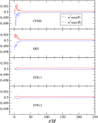
Even though our STP initial data do include realistic tidal deformations, they do so only approximately. On the other hand, CFMS and SKS initial data do not take into account the tidal deformations at all, so it is expected that their black hole geometries will be farther from equilibrium. This is confirmed in Fig. 3, which shows the extrema of $m^{2}\bar{R}$ over the surface of one black hole in the evolution of each initial data set. The horizon curvatures in the evolutions of CFMS and SKS initial data undergo similarly large variations at early times, but those for STP initial data are markedly smaller by about an order of magnitude. All the extrema are centered around the value of 0.5, that for a single Schwarzschild black hole.

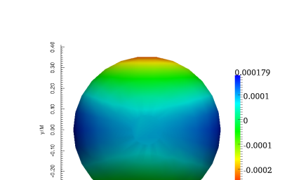
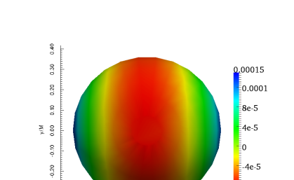
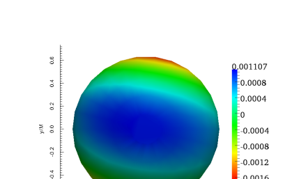
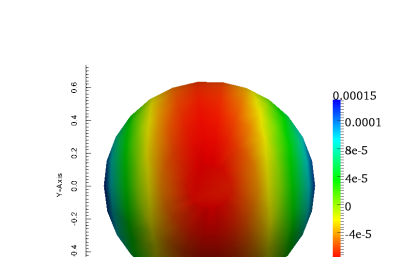
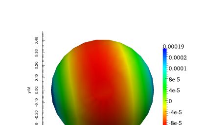
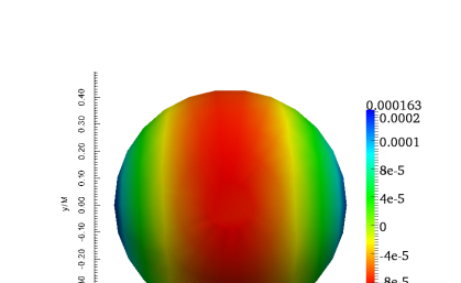
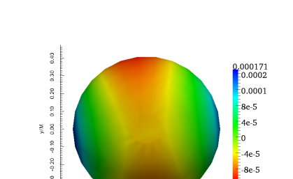
The values of $m^{2}\bar{R}$, minus the Schwarzschild value of 0.5, are plotted over the surfaces of the apparent horizons in Figs. 7 to 7 for a black hole in each initial data set, and for the same black hole at a time after relaxation, which we take to be $t_{\text{relaxed}}/M=250$. (The other black hole, which is not shown, is on the negative $x$-axis.) It is obvious that the black hole geometries in CFMS and SKS initial data do not represent their relaxed values. In contrast, the correct tidal deformations are much better captured in STP initial data.

Figure 9: Changes in the dimensionless spin $\chi(t)$ of a black hole relative to its starting value, during the evolution of different initial data sets. The vertical dashed line indicates a time $t_{\text{relaxed}}/M=250$ after relaxation.

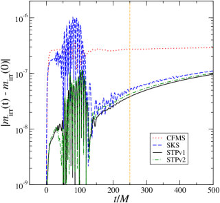
Changes in the black holes’ masses and spins are also induced by the initial relaxation. In Fig. 8, we show the difference in the irreducible mass from its initial value for a black hole in each evolution. The irreducible mass is defined as Hawking (1968)

$$m_{\text{irr}}(t)=\sqrt{A/16\pi},$$ (35)

where $A$ is the area of the apparent horizon. Near the time of relaxation $t_{\text{relaxed}}/M=250$, we see that going beyond conformal flatness with SKS initial data yields a noticeably smaller change in $m_{\text{irr}}(t)$ from its starting value. By including more realistic tidal deformations in our initial data, we can reduce this change slightly relative to SKS initial data. This is already evident with the inclusion of the Newtonian electric quadrupole in STPv2 initial data. By adding the higher-order pieces in STPv1 initial data, we achieve another slight improvement.

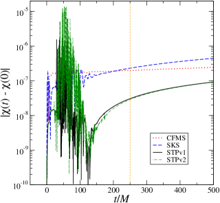
In Fig. 9, we show the difference in the dimensionless spin $\chi(t)$ of a black hole in each evolution, computed over the apparent horizon using approximate Killing vectors Lovelace et al. (2008), from its starting value. Unlike the mass, the change in $\chi(t)$ for SKS initial data is comparable to that for CFMS initial data at $t_{\text{relaxed}}/M=250$. In contrast, STP initial data show a clear improvement over the others. By adding pieces of the tidal fields beyond the Newtonian electric quadrupole though, the change in $\chi(t)$ for STPv1 initial data is a bit larger than for STPv2 initial data. This could be due to the corotating time dependence of the tidal fields that was used in STPv2 initial data, whereas STPv1 initial data only included the linearized time dependence.

Figure 10: Junk radiation generated in the evolutions of different initial data sets, shown for the $\left(l=2,m\geq 0\right)$ modes of $r_{\text{extr}}M\left|\Psi_{4}^{lm}\right|$ extracted at $r_{\text{extr}}/M=450$.

It is interesting that while the rates of change in $m_{\text{irr}}(t)$ and $\chi(t)$ are similar after relaxation for SKS and STP initial data, the rate for CFMS initial data is more gradual. This may be caused by the particular nature of junk radiation arising from these types of initial data, such as where it predominantly originates and how much is ingoing or outgoing. A comparison of these rates with post-Newtonian predictions of tidal heating would also give further insight Taylor and Poisson (2008). We quantify the amount of junk radiation generated in each initial data set in the next subsection, although determining their more detailed features requires further study.

Figure 11: Junk radiation generated in the evolutions of different initial data sets, shown for the $\left(l=3,m\geq 0\right)$ modes of $r_{\text{extr}}M\left|\Psi_{4}^{lm}\right|$ extracted at $r_{\text{extr}}/M=450$.

III.2 Junk radiation

At the beginning of an evolution, the entire spacetime geometry relaxes, and not just in the vicinity of the black holes. In the process, physically unrealistic gravitational radiation, or junk radiation, is generated. This junk radiation also contributes to the changes in the black holes discussed above. Here we compute and quantify the amount of junk radiation that develops for each initial data set.

Gravitational waves are extracted from the simulation on spheres of coordinate radius $r_{\text{extr}}$, following the same procedure in Boyle et al. (2007). We compute the Newman-Penrose scalar $\Psi_{4}$ given by

$$\Psi_{4}=-C_{\alpha\mu\beta\nu}l^{\mu}l^{\nu}\bar{m}^{\alpha}\bar{m}^{\beta},$$ (36)

where $C_{\alpha\beta\gamma\delta}$ is the Weyl curvature tensor, and

$$l^{\mu} =\frac{1}{\sqrt{2}}\left(n^{\mu}-r^{\mu}\right),$$ (37)

$$\bar{m}^{\mu} =\frac{1}{\sqrt{2}r}\left(\frac{\partial}{\partial\theta}-i\frac{1}{\sin\theta}\frac{\partial}{\partial\phi}\right)^{\mu},$$ (38)

in terms of spherical coordinates $\left(r,\theta,\phi\right)$ in the inertial frame, the timelike unit normal $n^{\mu}$ to the spatial hypersurface $\Sigma_{t}$, and the outward-pointing unit normal $r^{\mu}$ to the extraction sphere. Then $\Psi_{4}$ is expanded in terms of spin-weighted spherical harmonics of weight $-2$,

$$\Psi_{4}\left(t,r,\theta,\phi\right)=\displaystyle\sum_{lm}\Psi_{4}^{lm}\left(t,r\right)_{-2}Y_{lm}\left(\theta,\phi\right),$$ (39)

with expansion coefficients $\Psi_{4}^{lm}$.

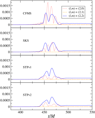
The burst of junk radiation is visible at early times in $\Psi_{4}^{lm}$. We consider the junk radiation extracted at $r_{\text{extr}}/M=450$. This is shown in Fig. 10 for the $\left(l=2,m\geq 0\right)$ modes of $r_{\text{extr}}M\left|\Psi_{4}^{lm}\right|$. For CFMS initial data, the largest component of the junk radiation is the $\left(2,0\right)$ mode. However, this mode is reduced by a factor of $\sim$2 each time, as we go to SKS and then to STP initial data. For SKS initial data, the magnitudes of the $\left(2,2\right)$ and $\left(2,0\right)$ modes are comparable. For both STPv1 and STPv2 initial data, the magnitude of the $\left(2,0\right)$ mode is $\sim$2 times smaller than for the $\left(2,2\right)$ mode. There is no substantial reduction in the $\left(2,2\right)$ mode of the junk radiation for either SKS or STP initial data though. This is not surprising, since the $\left(2,2\right)$ mode has a lower frequency and is thought to be associated with the lack of outgoing gravitational radiation in the initial data, which is an issue present in all of our initial data sets.

Figure 12: Junk radiation generated in the evolutions of different initial data sets, shown for the $\left(l=4,m\geq 0\right)$ modes of $r_{\text{extr}}M\left|\Psi_{4}^{lm}\right|$ extracted at $r_{\text{extr}}/M=450$.

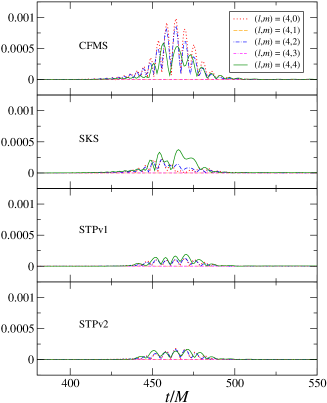
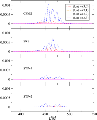
Evidently, including realistic tidal deformations is more effective at reducing the higher frequency modes of the junk radiation caused by the initial ringing of the black holes. This is further illustrated for the $\left(l=3,m\geq 0\right)$ modes in Fig. 11. There is a moderate reduction in the $\left(3,2\right)$ mode for SKS initial data over CFMS initial data, although there is no appreciable improvement for the $\left(3,0\right)$ mode. However, the $\left(3,2\right)$ mode for STP initial data is reduced by a factor of $\sim$4, and the $\left(3,0\right)$ mode by a factor of $\sim$2. A similar trend is seen for the $l=4$ modes in Fig. 12, but in this case the decrease in junk radiation for SKS initial data over CFMS initial data is much more obvious. Again, there are no major differences between STPv1 and STPv2 initial data.

Figure 13: Total junk radiation generated in the evolutions of different initial data sets, shown for the $\left(l=2,m\geq 0\right)$ and $\left(8\geq l\geq 3,m\geq 0\right)$ modes of $r_{\text{extr}}M\left|\Psi_{4}^{lm}\right|$ extracted at $r_{\text{extr}}/M=450$.

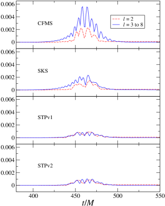
To examine the other higher-order modes in the junk radiation, we show the total contribution in the $\left(8\geq l\geq 3,m\geq 0\right)$ modes in Fig. 13. We also plot the total contribution in only the $\left(l=2,m\geq 0\right)$ modes for comparison. For both CFMS and SKS initial data, the combined junk radiation content in the higher-order modes is actually greater than in the $l=2$ modes alone, indicating the relevance of taking them into consideration. With our STP initial data, the situation is ameliorated, with the higher-order modes of the junk radiation being about the same magnitude as the $l=2$ modes. Simultaneously, both portions of the junk radiation are less than for CFMS and SKS initial data.

As a measure of the cumulative junk radiation content, we integrate the quantities in Fig. 13 over the time interval shown, $380M\leq t\leq 550M$, to obtain

$$I_{2} :=\int_{380M}^{550M}\sum\limits_{m=0}^{2}r_{\text{extr}}M\left|\Psi_{4}^{2m}\right|dt,$$ (40)

$$I_{3+} :=\int_{380M}^{550M}\sum\limits_{l=3}^{8}\sum\limits_{m=0}^{l}r_{\text{extr}}M\left|\Psi_{4}^{lm}\right|dt.$$ (41)

(An alternative would be to calculate the energy in the junk radiation, but we use this simpler measure here.) Their values are displayed in Table 2. The error estimates in $I_{2}$ and $I_{3+}$ are computed from the differences between the highest two resolutions, N2 and N3. For SKS initial data, $I_{2}$ is less by a factor of $\sim$1.4 and $I_{3+}$ is less by a factor of $\sim$2, relative to CFMS initial data. For both versions of STP initial data, $I_{2}$ is less by a factor of $\sim$1.7 and $I_{3+}$ is less by a factor of $\sim$5. They do differ somewhat from each other though, with $I_{2}$ a bit larger, and $I_{3+}$ a bit smaller, for STPv1 initial data. This again may be related to the different time dependences used in the tidal fields for the two cases.

Initial data	$\bm{I_{2}}$	$\bm{I_{3+}}$
CFMS	$0.050\pm 0.002$	$0.129\pm 0.004$
SKS	$0.0359\pm 0.0001$	$0.064\pm 0.002$
STPv1	$0.0294\pm 0.0002$	$0.0251\pm 0.0002$
STPv2	$0.0286\pm 0.0001$	$0.0270\pm 0.0001$

Table 2: Cumulative junk radiation content in the $\left(l=2,m\geq 0\right)$ modes $I_{2}$, and in the $\left(8\geq l\geq 3,m\geq 0\right)$ modes $I_{3+}$, computed via Eqs. (40)–(41).

IV Discussion

We have made a first attempt to include realistic tidal deformations in constraint-satisfying binary black-hole initial data, with the goal of understanding their effects on the relaxation of horizon properties, and the development of junk radiation in subsequent evolutions. This was done by superposing tidally perturbed black hole metrics as the conformal metric, in which the tidal fields were determined by asymptotically matching to a PN near zone metric Johnson-McDaniel et al. (2009). The results from evolutions were contrasted with those obtained with the widespread choice of conformally flat initial data, and those with initial data constructed by superposing Kerr-Schild metrics.

By more accurately representing the horizon geometries in our initial data, we found that the black holes’ intrinsic scalar curvatures deviated much less from their starting values at early times, with a corresponding decrease in the changes in the masses and spins. Past studies Kelly et al. (2010); Reifenberger and Tichy (2012), also considering equal-mass and nonspinning black holes, have focused on the impact of including PN corrections on the dominant $\left(2,2\right)$ mode of the relaxed binary. Here we have demonstrated that the total amount of junk radiation in the higher-order modes actually exceeds that in the $l=2$ modes alone, if one neglects realistic tidal deformations. With our STP initial data though, the junk radiation content in the higher-order modes becomes less than that in the $l=2$ modes, which is itself lowered. Thus, a more careful treatment of the horizons is not an inconsequential part of reducing junk radiation.

We constructed two versions of initial data with realistic tidal deformations, STPv1 that included all the tidal fields of Eqs. (44)–(47), and STPv2 that included only the Newtonian electric quadrupole but with a corotating time dependence given by Eqs. (29)–(30). Both of these versions gave very similar results for the early relaxation of the black holes, and the amount of junk radiation generated. This suggests that incorporating only the lowest-order tidal fields may be an adequate treatment of the horizons, in the absence of further refinements to other parts of the spacetime geometry. Moreover, this lends support to the effectiveness of using the tidally perturbed spinning metrics of Gallouin et al. (2012), which only have the lowest-order tidal fields. In Table 2, we also see that the cumulative junk radiation content in the $l=2$ modes is slightly larger for STPv1 initial data, but slightly smaller in the higher-order modes. Perhaps this indicates that our STPv1 initial data will benefit by using a corotating time dependence of the tidal fields instead.

There are still many potential avenues to improve upon our initial data. For instance, the superposition method itself limits how closely we are able to model the tidal deformations, because the Gaussian functions artificially alter the black hole metrics, and lead to unwanted perturbations of the horizon geometries. To overcome this, more sophisticated functions could be experimented with in the superposition, such as transition functions that satisfy the so-called Frankenstein theorems Yunes (2007).

Two of the most obvious shortcomings of our current initial data are the lack of outgoing gravitational radiation from the past history of the binary, and the absence of any interaction terms in the conformal metric for the region between the black holes. In fact, these were already accounted for in the approximate initial data of Johnson-McDaniel et al. (2009), which can be directly supplied as conformal data to solve for the Einstein constraint equations. This work is currently in progress Throwe et al. .

It is straightforward to generalize our tidally perturbed initial data to unequal-mass binaries. Since the PN approximation is known to be less accurate in this regime MacDonald et al. (2013), assuming the same binary separation, it would be interesting to see how well the results compare to the ones presented here. The effects of spin can also be investigated with the black hole metrics of Gallouin et al. (2012). As mentioned earlier, we may also be able to reduce the eccentricity by adjusting the free parameters in the superposition functions, the metrics in Cook-Scheel coordinates, and the accompanying coordinate transformation to PN harmonic coordinates. Our initial data can then be combined with the iterative prescription of Zhang and Szilágyi (2013) to jointly diminish junk radiation and eccentricity. Finally, since our waveforms were extracted at a finite radius, they inevitably contain gauge effects. We have compared the junk radiation content for waveforms extracted at different radii, and find no significant differences. Nevertheless, it might be worthwhile to analyze the junk radiation with these effects removed through Cauchy-characteristic extraction, for instance Winicour (2009); Taylor et al. (2013).

Appendix A Tidally perturbed black hole metrics from asymptotic matching

The exact expressions from Johnson-McDaniel et al. (2009) that we use to construct our superposed tidally-perturbed initial data are collected here for completeness. For all equations in this appendix, indices are raised and lowered with the flat spacetime metric $\eta_{\mu\nu}$. One begins with a perturbed Schwarzschild metric in Cook-Scheel harmonic coordinates $X^{\mu}=\left(T,X^{i}\right)$ Cook and Scheel (1997), comoving with and centered on that black hole,

$$h_{\mu\nu}dX^{\mu}dX^{\nu} =-H_{T^{2}}dT^{2}+H_{RT}dRdT+\frac{16}{3}\frac{\tilde{M}^{2}}{R}\left[1+\frac{\tilde{M}}{R}-\frac{2}{3}\frac{\tilde{M}^{3}}{R^{2}(R+\tilde{M})}\right]\dot{{\mathcal{C}}}_{klp}X^{l}X^{p}dX^{k}dT$$

$$\quad+H_{k}^{[1]}dX^{k}\left[\left(1-\frac{\tilde{M}^{2}}{R^{2}}\right)dT-4\frac{\tilde{M}^{2}}{R^{2}}dR\right]+H_{k}^{[2]}dX^{k}dR+H_{R^{2}}dR^{2}+H_{\text{trc}}dX_{s}dX^{s},$$

$$\quad+{\mathcal{O}}(R^{4}/{\mathcal{R}}^{4}),$$ (42)

where $R:=\sqrt{X_{i}X^{i}}$ and the metric functions are

$$H_{T^{2}} =\frac{R-\tilde{M}}{R+\tilde{M}}+\left[1-\frac{\tilde{M}}{R}\right]^{2}\left[({\mathcal{E}}_{kl}+T\dot{{\mathcal{E}}}_{kl})X^{k}X^{l}+\frac{1}{3}{\mathcal{E}}_{klp}X^{k}X^{l}X^{p}\right]$$

$$\quad+\frac{4\tilde{M}^{2}}{(R+\tilde{M})^{2}}\left[R-\frac{5}{3}\frac{\tilde{M}^{2}}{R}\right]\dot{{\mathcal{E}}}_{kl}X^{k}X^{l},$$

$$H_{RT} =\frac{8\tilde{M}^{2}}{(R+\tilde{M})^{2}}+8\frac{\tilde{M}^{2}}{R^{2}}\frac{R-\tilde{M}}{R+\tilde{M}}\left[({\mathcal{E}}_{kl}+T\dot{{\mathcal{E}}}_{kl})X^{k}X^{l}+\frac{1}{3}{\mathcal{E}}_{klp}X^{k}X^{l}X^{p}\right]$$

$$\quad-\left[\frac{4}{3}R+\frac{14}{3}\tilde{M}+\frac{8}{3}\frac{\tilde{M}^{2}}{R}-2\frac{\tilde{M}^{3}}{R^{2}}-\frac{104}{3}\frac{\tilde{M}^{4}}{R^{2}(R+\tilde{M})}+\frac{80}{3}\frac{\tilde{M}^{5}}{R^{2}(R+\tilde{M})^{2}}\right.$$

$$\left.\quad\quad+\frac{32}{3}\frac{\tilde{M}^{6}}{R^{2}(R+\tilde{M})^{3}}\right]\dot{{\mathcal{E}}}_{kl}X^{k}X^{l},$$

$$H_{k}^{[1]} =\frac{2}{3}\left[1+\frac{\tilde{M}}{R}\right]\left[2({\mathcal{C}}_{klp}+T\dot{{\mathcal{C}}}_{klp})X^{l}X^{p}+\left(1-\frac{1}{3}\frac{\tilde{M}}{R}\right){\mathcal{C}}_{klps}X^{l}X^{p}X^{s}\right],$$ (43)

$$H_{k}^{[2]} =\left[\frac{R}{3}+2\tilde{M}+\frac{16}{3}\frac{\tilde{M}^{2}}{R}+\frac{26}{3}\frac{\tilde{M}^{3}}{R^{2}}-11\frac{\tilde{M}^{4}}{R^{3}}-\frac{32}{3}\frac{\tilde{M}^{5}}{R^{3}(R+\tilde{M})}-\frac{64}{9}\frac{\tilde{M}^{6}}{R^{3}(R+\tilde{M})^{2}}\right]\dot{{\mathcal{C}}}_{klp}X^{l}X^{p},$$

$$H_{R^{2}} =\sum_{n=1}^{3}\left(\frac{2\tilde{M}}{R+\tilde{M}}\right)^{n}-\frac{2\tilde{M}}{R}-\frac{\tilde{M}^{2}}{R^{2}}+\left[2\frac{\tilde{M}}{R}+3\frac{\tilde{M}^{2}}{R^{2}}-\frac{\tilde{M}^{4}}{R^{4}}-\frac{16\tilde{M}^{4}}{R^{2}(R+\tilde{M})^{2}}\right]({\mathcal{E}}_{kl}+T\dot{{\mathcal{E}}}_{kl})X^{k}X^{l},$$

$$\quad+\left[\frac{1}{3}\frac{\tilde{M}}{R}+\frac{1}{3}\frac{\tilde{M}^{2}}{R^{2}}-\frac{2}{5}\frac{\tilde{M}^{3}}{R^{3}}-\frac{7}{15}\frac{\tilde{M}^{4}}{R^{4}}-\frac{1}{15}\frac{\tilde{M}^{5}}{R^{5}}-\frac{16}{3}\frac{\tilde{M}^{4}}{R^{2}(R+\tilde{M})^{2}}\right]{\mathcal{E}}_{klp}X^{k}X^{l}X^{p}$$

$$\quad+\left[\frac{16}{3}\frac{\tilde{M}^{2}}{R}+\frac{80}{3}\frac{\tilde{M}^{3}}{R^{2}}+28\frac{\tilde{M}^{4}}{R^{3}}+\frac{40}{3}\frac{\tilde{M}^{5}}{R^{4}}-\frac{176}{3}\frac{\tilde{M}^{6}}{R^{4}(R+\tilde{M})}+\frac{72\tilde{M}^{7}}{R^{4}(R+\tilde{M})^{2}}\right.$$

$$\left.\quad\quad-\frac{32}{3}\frac{\tilde{M}^{8}}{R^{4}(R+\tilde{M})^{3}}-\frac{32}{3}\frac{\tilde{M}^{9}}{R^{4}(R+\tilde{M})^{4}}\right]\dot{{\mathcal{E}}}_{kl}X^{k}X^{l},$$

$$H_{\text{trc}} =\left[1+\frac{\tilde{M}}{R}\right]^{2}\left[1-\left(1+2\frac{\tilde{M}}{R}-\frac{\tilde{M}^{2}}{R^{2}}\right)({\mathcal{E}}_{kl}+T\dot{{\mathcal{E}}}_{kl})X^{k}X^{l}\right.$$

$$\left.\quad-\frac{1}{3}\left(1+\frac{\tilde{M}}{R}-\frac{\tilde{M}^{2}}{R^{2}}-\frac{1}{5}\frac{\tilde{M}^{3}}{R^{3}}\right){\mathcal{E}}_{klp}X^{k}X^{l}X^{p}-4\frac{\tilde{M}^{2}}{R^{2}}\left(R+2\tilde{M}-\frac{2}{3}\frac{\tilde{M}^{2}}{R+\tilde{M}}\right)\dot{{\mathcal{E}}}_{kl}X^{k}X^{l}\right],$$

and $\mathcal{R}$ is the characteristic length scale of the perturbation (see below). The electric quadrupole and octupole tidal fields are denoted by ${\mathcal{E}}_{kl}$ and ${\mathcal{E}}_{klp}$, respectively. The magnetic quadrupole and octupole tidal fields are similarly denote by ${\mathcal{B}}_{kl}$ and ${\mathcal{B}}_{klp}$, respectively. They enter Eq. (A) through ${\mathcal{C}}_{klp}=\epsilon_{kls}{\mathcal{B}}^{s}_{p}$ and ${\mathcal{C}}_{klps}=\epsilon_{klu}{\mathcal{B}}^{u}_{ps}$, where $\epsilon_{ijk}$ is the spatial Levi-Civita symbol. The overdots on the tidal fields denote time derivatives. Note that $h_{\mu\nu}$ is formally only applicable for small $R$, since the metric functions in Eq. (A) contain terms that diverge as $R\rightarrow\infty$.

Next consider an $\mathcal{O}\left(v^{4}\right)$ PN metric Blanchet et al. (1998) in barycentric harmonic coordinates $x^{\mu}=\left(t,x^{i}\right)$ and specialized to a circular orbit, for which at $t=0$ one black hole (“hole 1”) of mass $\tilde{m}_{1}$ lies along the positive $x$-axis and the other black hole (“hole 2”) of mass $\tilde{m}_{2}$ lies along the negative $x$-axis. By asymptotically matching the perturbed Schwarzschild and PN metrics, the tidal fields about hole 1 are given by

$${\mathcal{E}}_{kl}(t) =\frac{\tilde{m}_{2}}{b^{3}}\left\{\left[1-\frac{1}{2}\frac{\tilde{m}_{2}}{b}\right][\delta_{kl}-3\hat{x}_{k}\hat{x}_{l}]+\frac{1}{2}\frac{\tilde{m}}{b}[4\hat{x}_{k}\hat{x}_{l}-5\hat{y}_{k}\hat{y}_{l}+\hat{z}_{k}\hat{z}_{l}]-6\sqrt{\frac{\tilde{m}}{b}}\frac{t}{b}\hat{x}_{(k}\hat{y}_{l)}\right\},$$ (44)

$${\mathcal{B}}_{kl}(t) =\frac{\tilde{m}_{2}}{b^{3}}\sqrt{\frac{\tilde{m}_{2}}{b}}\left\{\left[-6\sqrt{\frac{\tilde{m}}{\tilde{m}_{2}}}+\frac{\tilde{m}_{2}}{b}\left\{5\left(\frac{\tilde{m}}{\tilde{m}_{2}}\right)^{3/2}+7\sqrt{\frac{\tilde{m}}{\tilde{m}_{2}}}-3\sqrt{\frac{\tilde{m}_{2}}{\tilde{m}}}\right\}\right]\hat{x}_{(k}\hat{z}_{l)}\right.$$

$$\left.\quad-6\frac{\tilde{m}}{\tilde{m}_{2}}\sqrt{\frac{\tilde{m}_{2}}{b}}\frac{t}{b}\hat{y}_{(k}\hat{z}_{l)}\right\},$$ (45)

$${\mathcal{E}}_{klp}(t) =\frac{\tilde{m}_{2}}{b^{4}}\left\{\left[1-3\frac{\tilde{m}_{2}}{b}\right][15\hat{x}_{k}\hat{x}_{l}\hat{x}_{p}-9\delta_{(kl}\hat{x}_{p)}]-3\frac{\tilde{m}}{b}[\hat{x}_{k}\hat{x}_{l}\hat{x}_{p}-4\hat{y}_{(k}\hat{y}_{l}\hat{x}_{p)}+\hat{z}_{(k}\hat{z}_{l}\hat{x}_{p)}]\right\},$$ (46)

$${\mathcal{B}}_{klp}(t) =\frac{9}{2}\frac{\tilde{m}_{2}}{b^{4}}\sqrt{\frac{\tilde{m}}{b}}\left[5\hat{x}_{(k}\hat{x}_{l}\hat{z}_{p)}-\delta_{(kl}\hat{z}_{p)}\right],$$ (47)

where $\tilde{m}=\tilde{m}_{1}+\tilde{m}_{2}$, $b$ is the PN coordinate separation of the holes, and $\hat{x}^{\mu},\hat{y}^{\mu}$, $\hat{z}^{\mu}$ (and $\hat{t}^{\mu}$ below, with $\hat{t}_{0}=-1$) are Cartesian basis vectors. In the region around hole 1, the characteristic length scale of the perturbation in Eq. (A) is ${\mathcal{R}}\sim\sqrt{b^{3}/m_{2}}$ Thorne and Hartle (1985). The tidal fields about hole 2 are obtained by letting $\tilde{m}_{2}\rightarrow\tilde{m}_{1}$, $\hat{x}_{\mu}\rightarrow-\hat{x}_{\mu}$, and $\hat{y}_{\mu}\rightarrow-\hat{y}_{\mu}$. These tidal fields are only valid for times $t\approx 0$.

Finally, the perturbed Schwarzschild metrics are transformed to PN harmonic coordinates (only up to $\mathcal{O}\left(v^{3}\right)$ here), which around hole 1 is given by

$$X^{\alpha}(x^{\beta})=\sum_{j=0}^{3}\left(\frac{\tilde{m}_{2}}{b}\right)^{j/2}\left(X^{\alpha}\right)_{j}(x^{\beta})+{\mathcal{O}}\left(v^{4}\right),$$ (48)

where

$$\left(X_{\alpha}\right)_{0} =x_{\alpha}+\left(\tilde{m}_{2}/\tilde{m}\right)b\hat{x}_{\alpha},$$ (49)

$$\left(X_{\alpha}\right)_{1} =\left(F_{\beta\alpha}\right)_{1}\tilde{x}^{\beta},$$ (50)

$$\left(X_{\alpha}\right)_{2} =\left[1-\frac{\tilde{x}}{b}\right]\Delta_{\alpha\beta}\tilde{x}^{\beta}+\frac{\Delta_{\beta\gamma}\tilde{x}^{\beta}\tilde{x}^{\gamma}}{2b}\hat{x}_{\alpha}$$

$$-\frac{1}{2}\left(F_{\alpha}^{\;\gamma}\right)_{1}\left(F_{\beta\gamma}\right)_{1}\tilde{x}^{\beta},$$ (51)

$$\left(X_{\alpha}\right)_{3} =\sqrt{\frac{\tilde{m}}{\tilde{m}_{2}}}\left\{-\frac{yt}{b^{2}}\Delta_{\alpha\beta}\tilde{x}^{\beta}+\left[\frac{\tilde{x}_{\mu}\tilde{x}^{\mu}-4\tilde{x}^{2}}{2b^{2}}\right.\right.$$

$$\quad\left.+\left(2-\frac{\tilde{m}_{2}}{\tilde{m}}\right)\frac{\tilde{x}}{b}+\left(2+\frac{1}{2}\frac{\tilde{m}_{2}}{\tilde{m}}\right)\frac{\tilde{m}_{2}}{\tilde{m}}\right]y\hat{t}_{\alpha}$$

$$\quad\left.+2\left[1-\frac{\tilde{m}_{2}}{\tilde{m}}\right]\frac{yt}{b}\hat{x}_{\alpha}+\left[\frac{3\tilde{r}^{2}+t^{2}}{6b^{2}}\right.\right.$$

$$\quad\left.\left.+\left(\frac{\tilde{m}_{2}}{\tilde{m}}-2\right)\frac{\tilde{x}}{b}+\frac{1}{2}\left(\frac{\tilde{m}_{2}}{\tilde{m}}\right)^{2}+4\right]t\hat{y}_{\alpha}\right\}$$

$$\quad+\left(F_{\beta\alpha}\right)_{3}\tilde{x}^{\beta}+\frac{1}{2b^{3}}\sqrt{\frac{\tilde{m}}{\tilde{m}_{2}}}\tilde{x}y\left(4\tilde{x}^{2}-y^{2}-z^{2}\right)\hat{t}_{\alpha}.$$ (52)

In the above, $\tilde{x}^{\alpha}:=x^{\alpha}-\left(\tilde{m}_{2}/\tilde{m}\right)b\hat{x}^{\alpha}$, $\tilde{x}:=x-\left(\tilde{m}_{2}/\tilde{m}\right)b$, $\tilde{r}:=\sqrt{\tilde{x}_{k}\tilde{x}^{k}}$, $\Delta_{\alpha\beta}:=\text{diag}\left(1,1,1,1\right)$, and

$$\left(F_{\alpha\beta}\right)_{1} =2\sqrt{\frac{\tilde{m}_{2}}{\tilde{m}}}\hat{t}_{[\alpha}\hat{y}_{\beta]},$$ (53)

$$\left(F_{\alpha\beta}\right)_{3} =\left[\left(\frac{\tilde{m}_{2}}{\tilde{m}}\right)^{3/2}+3\sqrt{\frac{\tilde{m}_{2}}{\tilde{m}}}+5\sqrt{\frac{\tilde{m}}{\tilde{m}_{2}}}\right]\hat{t}_{[\alpha}\hat{y}_{\beta]},$$ (54)

encode the parts of the hole’s Lorentz boost that are determined by the matching. The coordinate transformation around hole 2 is obtained from the preceding expressions by making the substitutions $\tilde{m}_{1}\rightarrow\tilde{m}_{2}$, $\left(t,x,y,z\right)\rightarrow\left(t,-x,-y,z\right)$, and $\left(T,X,Y,Z\right)\rightarrow\left(T,-X,-Y,Z\right)$.

References

- et al. (2006) B. A. et al. (LIGO Scientific Collaboration), Phys. Rev. D 73, 062001 (2006).
- di Fiore (2002) L. di Fiore (VIRGO), Class. Quantum Grav. 19, 1421 (2002).
- Garat and Price (2000) A. Garat and R. H. Price, Phys. Rev. D 61, 124011 (2000).
- Valiente Kroon (2004) J. A. Valiente Kroon, Class. Quantum Grav. 21, 3237 (2004).
- Nissanke (2006) S. Nissanke, Phys. Rev. D 73, 124002 (2006).
- Boyle et al. (2007) M. Boyle, D. A. Brown, L. E. Kidder, A. H. Mroué, H. P. Pfeiffer, M. A. Scheel, G. B. Cook, and S. A. Teukolsky, Phys. Rev. D 76, 124038 (2007).
- Hannam et al. (2008) M. Hannam, S. Husa, J. A. González, U. Sperhake, and B. Brügmann, Phys. Rev. D 77, 044020 (2008).
- Zlochower et al. (2012) Y. Zlochower, M. Ponce, and C. O. Lousto, Phys. Rev. D 86, 104056 (2012).
- Postnov and Yungelson (2005) K. Postnov and L. Yungelson, Living Rev. Rel. 9, 6 (2005), eprint astro-ph/0701059.
- Zhang and Szilágyi (2013) F. Zhang and B. Szilágyi, Phys. Rev. D 88, 084033 (2013).
- Matzner et al. (1998) R. A. Matzner, M. F. Huq, and D. Shoemaker, Phys. Rev. D 59, 024015 (1998).
- Marronetti and Matzner (2000) P. Marronetti and R. A. Matzner, Phys. Rev. Lett. 85, 5500 (2000).
- Marronetti et al. (2000) P. Marronetti, M. Huq, P. Laguna, L. Lehner, R. A. Matzner, and D. Shoemaker, Phys. Rev. D 62, 024017 (2000).
- Hannam et al. (2007) M. Hannam, S. Husa, B. Brügmann, J. A. Gonzalez, and U. Sperhake, Class. Quantum Grav. 24, S15 (2007), eprint gr-qc/0612001.
- Lovelace et al. (2008) G. Lovelace, R. Owen, H. P. Pfeiffer, and T. Chu, Phys. Rev. D 78, 084017 (2008).
- Lovelace (2009) G. Lovelace, Class. Quantum Grav. 26, 114002 (2009).
- Blanchet (2006) L. Blanchet, Living Rev.Rel. 9, 4 (2006).
- Kelly et al. (2007) B. J. Kelly, W. Tichy, M. Campanelli, and B. F. Whiting, Phys. Rev. D 76, 024008 (2007).
- Kelly et al. (2010) B. J. Kelly, W. Tichy, Y. Zlochower, M. Campanelli, and B. Whiting, Class. Quantum Grav. 27, 114005 (2010).
- Mundim et al. (2011) B. C. Mundim, B. J. Kelly, Y. Zlochower, H. Nakano, and M. Campanelli, Class. Quantum Grav. 28, 134003 (2011).
- Johnson-McDaniel et al. (2009) N. K. Johnson-McDaniel, N. Yunes, W. Tichy, and B. J. Owen, Phys.Rev. D80, 124039 (2009), eprint 0907.0891.
- Gallouin et al. (2012) L. Gallouin, H. Nakano, N. Yunes, and M. Campanelli, Class. Quantum Grav. 29, 235013 (2012), eprint arXiv:1208.6489.
- Yunes et al. (2006) N. Yunes, W. Tichy, B. J. Owen, and B. Brügmann, Phys. Rev. D 74, 104011 (2006).
- Yunes and Tichy (2006) N. Yunes and W. Tichy, Phys. Rev. D 74, 064013 (2006).
- Reifenberger and Tichy (2012) G. Reifenberger and W. Tichy, Phys. Rev. D 86, 064003 (2012), URL http://link.aps.org/doi/10.1103/PhysRevD.86.064003.
- Pfeiffer et al. (2003) H. P. Pfeiffer, L. E. Kidder, M. A. Scheel, and S. A. Teukolsky, Comput. Phys. Commun. 152, 253 (2003).
- Szilagyi et al. (2009) B. Szilagyi, L. Lindblom, and M. A. Scheel, Phys. Rev. D 80, 124010 (2009), eprint 0909.3557.
- York (1999) J. W. York, Phys. Rev. Lett. 82, 1350 (1999).
- Pfeiffer and York (2003) H. P. Pfeiffer and J. W. York, Phys. Rev. D 67, 044022 (2003).
- Arnowitt et al. (1962) R. Arnowitt, S. Deser, and C. W. Misner, in Gravitation: An Introduction to Current Research, edited by L. Witten (Wiley, New York, 1962).
- York, Jr. (1979) J. W. York, Jr., in Sources of Gravitational Radiation, edited by L. L. Smarr (Cambridge University Press, Cambridge, England, 1979), pp. 83–126.
- Bowen and York, Jr. (1980) J. M. Bowen and J. W. York, Jr., Phys. Rev. D 21, 2047 (1980).
- M. Scheel, M. Boyle, T. Chu, L. Kidder, K. Matthews and H. Pfeiffer (2009) M. Scheel, M. Boyle, T. Chu, L. Kidder, K. Matthews and H. Pfeiffer, Phys. Rev. D 79, 024003 (2009), eprint arXiv:gr-qc/0810.1767.
- Lichnerowicz (1944) A. Lichnerowicz, J. Math Pures et Appl. 23, 37 (1944).
- Smarr and York (1978) L. Smarr and J. W. York, Phys. Rev. D 17, 2529 (1978).
- Cook and Pfeiffer (2004) G. B. Cook and H. P. Pfeiffer, Phys. Rev. D 70, 104016 (2004).
- Caudill et al. (2006) M. Caudill, G. B. Cook, J. D. Grigsby, and H. P. Pfeiffer, Phys. Rev. D 74, 064011 (2006).
- Pfeiffer et al. (2007) H. P. Pfeiffer, D. A. Brown, L. E. Kidder, L. Lindblom, G. Lovelace, and M. A. Scheel, Class. Quantum Grav. 24, S59 (2007).
- Lovelace et al. (2012) G. Lovelace, M. Boyle, M. A. Scheel, and B. Szilágyi, Class.Quant.Grav. 29, 045003 (2012), eprint arXiv:1110.2229.
- Cook and Scheel (1997) G. B. Cook and M. A. Scheel, Phys. Rev. D 56, 4775 (1997).
- Blanchet et al. (1998) L. Blanchet, G. Faye, and B. Ponsot, Phys. Rev. D 58, 124002 (1998).
- Booth (2005) I. Booth, Can. J. Phys. 83, 1073 (2005), eprint gr-qc/0508107.
- Johnson-McDaniel (2012) N. K. Johnson-McDaniel, private communication (2012).
- Scheel et al. (2006) M. A. Scheel, H. P. Pfeiffer, L. Lindblom, L. E. Kidder, O. Rinne, and S. A. Teukolsky, Phys. Rev. D 74, 104006 (2006).
- (45) http://www.black-holes.org/SpEC.html.
- Lindblom et al. (2006) L. Lindblom, M. A. Scheel, L. E. Kidder, R. Owen, and O. Rinne, Class. Quantum Grav. 23, S447 (2006).
- Friedrich (1985) H. Friedrich, Commun. Math. Phys. 100, 525 (1985).
- Garfinkle (2002) D. Garfinkle, Phys. Rev. D 65, 044029 (2002).
- Pretorius (2005) F. Pretorius, Class. Quantum Grav. 22, 425 (2005).
- Rinne (2006) O. Rinne, Class. Quantum Grav. 23, 6275 (2006).
- Rinne et al. (2007) O. Rinne, L. Lindblom, and M. A. Scheel, Class. Quantum Grav. 24, 4053 (2007).
- Stewart (1998) J. M. Stewart, Class. Quantum Grav. 15, 2865 (1998).
- Friedrich and Nagy (1999) H. Friedrich and G. Nagy, Commun. Math. Phys. 201, 619 (1999).
- Bardeen and Buchman (2002) J. M. Bardeen and L. T. Buchman, Phys. Rev. D 65, 064037 (2002).
- Szilágyi et al. (2002) B. Szilágyi, B. Schmidt, and J. Winicour, Phys. Rev. D 65, 064015 (2002).
- Calabrese et al. (2003) G. Calabrese, J. Pullin, O. Reula, O. Sarbach, and M. Tiglio, Commun. Math. Phys. 240, 377 (2003), eprint gr-qc/0209017.
- Szilágyi and Winicour (2003) B. Szilágyi and J. Winicour, Phys. Rev. D 68, 041501(R) (2003).
- Kidder et al. (2005) L. E. Kidder, L. Lindblom, M. A. Scheel, L. T. Buchman, and H. P. Pfeiffer, Phys. Rev. D 71, 064020 (2005).
- Buchman and Sarbach (2006) L. T. Buchman and O. C. A. Sarbach, Class. Quantum Grav. 23, 6709 (2006).
- Buchman and Sarbach (2007) L. T. Buchman and O. C. A. Sarbach, Class. Quantum Grav. 24, S307 (2007).
- Gottlieb and Hesthaven (2001) D. Gottlieb and J. S. Hesthaven, J. Comput. Appl. Math. 128, 83 (2001), ISSN 0377-0427.
- Hesthaven (2000) J. S. Hesthaven, Appl. Num. Math. 33, 23 (2000).
- Lindblom et al. (2008) L. Lindblom, K. D. Matthews, O. Rinne, and M. A. Scheel, Phys. Rev. D 77, 084001 (2008).
- Hawking (1968) S. W. Hawking, J. Math. Phys. 9, 598 (1968).
- Taylor and Poisson (2008) S. Taylor and E. Poisson, Phys. Rev. D 78, 084016 (2008).
- Yunes (2007) N. Yunes, Class. Quantum Grav. 24, 4313 (2007), eprint 0611128.
- (67) W. Throwe et al., in preparation.
- MacDonald et al. (2013) I. MacDonald, A. H. Mroué, H. P. Pfeiffer, M. Boyle, L. E. Kidder, M. A. Scheel, B. Szilágyi, and N. W. Taylor, Phys. Rev. D 87, 024009 (2013), eprint 1210.3007.
- Winicour (2009) J. Winicour, Living Rev. Rel. 12 (2009), URL http://www.livingreviews.org/lrr-2009-3.
- Taylor et al. (2013) N. W. Taylor, M. Boyle, C. Reisswig, M. A. Scheel, T. Chu, et al. (2013), arXiv:1309.3605, eprint 1309.3605.
- Thorne and Hartle (1985) K. S. Thorne and J. B. Hartle, Phys. Rev. D 31, 1815 (1985).