Effects of External Radiation Fields on Line Emission — Application to Star-forming Regions

Abstract

A variety of astronomical environments contain clouds irradiated by a combination of isotropic and beamed radiation fields. For example, molecular clouds may be irradiated by the isotropic cosmic microwave background (CMB), as well as by a nearby active galactic nucleus (AGN). These radiation fields excite atoms and molecules and produce emission in different ways. We revisit the escape probability theorem and derive a novel expression that accounts for the presence of external radiation fields. We show that when the field is isotropic the escape probability is reduced relative to that in the absence of external radiation. This is in agreement with previous results obtained under ad hoc assumptions or with the two-level system, but can be applied to complex many-level models of atoms or molecules. This treatment is in the development version of the spectral synthesis code Cloudy. We examine the spectrum of a Spitzer cloud embedded in the local interstellar radiation field, and show that about 60 percent of its emission lines are sensitive to background subtraction. We argue that this geometric approach could provide an additional tool toward understanding the complex radiation fields of starburst galaxies.

1. Introduction

Emission-line clouds can be powered by a variety of external radiation fields. Examples include H ii regions powered by nearby stars or the diffuse interstellar medium (ISM) powered by the net emission of the surrounding galaxy. The angular distribution of the radiation that powers the cloud has little effect on the ionization or temperature of a cell of gas, but the radiation transport and net line emission can be quite different, and these affect the observed spectrum.

We have updated the plasma simulation code Cloudy, last reviewed by Ferland et al. (2013), to account for various types of external radiation fields. The fundamental distinction is between a “beamed” field, such as that produced by a single star or nearby AGN, versus a nearly isotropic field such as the CMB or a surrounding starburst.

In sections §§2–6 we derive the formalism needed to treat these two cases. The observed emission can be quite different when continuum pumping is important. In §7 we present an astrophysical application on the emission from the diffuse ISM, such as might be observed from regions of a starburst galaxy, and outline observational tests which can help determine the geometry of the radiation field that powers an astrophysical object. We conclude in §8.

2. An overview of escape probabilities

Figure 1 shows an idealized geometry of the process we consider. The observer is to the left and an isolated atom is at the center of the cavity. If collisional excitation can be neglected, then radiation from the surrounding walls is the only source of excitation. Assume for the moment that we can neglect stimulated emission produced by the external radiation field. Two possible photon paths are indicated. The solid line indicates the path of a photon which is initially directed towards the observer but is scattered away after absorption by the atom. This would produce an absorption line were no other photons present. The dashed line indicates the path of the photon initially directed transverse to the line of sight of the observer, but which is scattered towards the observer after encountering the atom. This would produce an emission line were no other photons present. In a fully symmetric geometry these two processes completely compensate. The atom experiences two excitations but the observer sees no net emission or absorption. The same conclusion holds when stimulated emission is taken into account. This is in contrast to a beamed continuum, in which an emission or absorption line is produced following each photo-excitation.

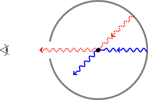
Figure 1.— An idealized geometry showing the cancellation that occurs with an isotropic radiation field. An atom is taken to lie at the center of a surrounding source of radiation. The observer is to the left. The solid (blue) line indicates a photon scattered away from the line of sight to the observer. The dashed (red) line indicates the path of a photon which is scattered into the line of sight, compensating for the loss of the original photon.

Collisions lead to emission or absorption lines against the background continuum according to Kirchhoff’s laws. Assuming that the intervening gas is hotter than the background continuum, as is the case for the CMB, the intensity of the emission line that will form will depend on the gas density. Compared to the case of no external radiation, the net line emissivity will be reduced. The diminution occurs because, although the radiation enhances the upper level population and therefore the emissivity, absorption along the line of sight is in excess of that gain. At the extreme where radiative transitions dominate, the level population density ratio should become equal to the Boltzmann ratio at the radiation temperature and no emission in excess of the continuum should be possible, as discussed above.

The remainder of this section provides an introduction to the escape probability theory and lays the groundwork for developments in later sections. The escape probability theorem is a commonly used approximation in radiative transfer. It is invoked to simplify the problem of photon propagation through a gaseous medium. In principle, photons generated at any point in the medium may be absorbed or scattered at some different point, or they may escape without undergoing further interactions. These potentially non-local couplings render the problem of photon transfer analytically, and in many cases even numerically, intractable.

The theorem states that the net number of photons created at some position in the medium in fact escapes without suffering any absorptions, leading to a great simplification of the problem. Although further assumptions need to be made regarding the non-escaping photons in order to reach a complete solution to a radiative transfer problem, the value of the escape probability theorem lies in that it decouples the radiative transfer and the local statistical state problems.

The first rigorous proof of the theorem is due to Irons (1978), who considered averages over a unit volume of a gas. Later, Rybicki (1984) showed that the theorem applies to individual rays of monochromatic radiation as well, that is, the theorem is much more detailed than was previously realized. Both derivations take into account the radiation field generated by the medium itself, the so-called diffuse field, but do not consider the effects of external radiation.

Previous work has included external fields in two fashions. First, in multi-level atomic models (e.g., Goldreich & Kwan, 1974) a term is introduced in the statistical state equations to account for the presence of external isotropic radiation. Alternatively, calculations that rely on the state of a two-level atom embedded in isotropic external radiation have employed a diminution factor for the emergent intensity. In the case of hyperfine structure lines, D’Cruz et al. (1998) and Sunyaev & Docenko (2007) have derived a factor of the form

$$D(\eta_{\nu},n_{e},n_{c})=\Bigl{\{}1+(1+g_{u}/g_{l})(\eta_{\nu}+n_{e}/n_{c})\Bigr{\}}^{-1}\,,$$ (1)

where $\eta_{\nu}$ is the photon occupation number at the line frequency, $g_{u}$ and $g_{l}$ are the statistical weights of the upper and lower states, $n_{e}$ is the electron density, and $n_{c}=A_{ul}/q_{ul}$ is the critical density, with $A_{ul}$ and $q_{ul}$ being the Einstein coefficient and the downward collisional rate coefficient, respectively. (Collisions are mainly induced by electron impact in these calculations.)

In this paper we extend previous proofs by explicitly accounting for external radiation fields, and arrive at a novel expression for the escape probability. Our expression is similar to that adopted by Goldreich & Kwan (1974), and leads to diminution factors consistent with D’Cruz et al. (1998) and Sunyaev & Docenko (2007). However, unlike the latter, our expression may be applied to systems for which the critical density may not be defined. In fact, in our implementation in the spectral code Cloudy (C13; Ferland et al., 2013), all transitions are handled uniformly, including those whose level populations stem from the solution of a multi-level model.

In §3 we present the basic equations of the two-level atom, while in §4 we introduce some key concepts of the escape probability theorem. Then, in §5 we derive the theorem in the presence of external radiation both along rays, as well as for volume averages. In §6 we discuss our implementation in Cloudy.

3. Two-level Atom

Although the derivation of the theorem is quite general, in the following we will adopt the forms of the two-level atom for convenience. It should be understood, however, that the levels referred to below are the upper and lower levels associated with any line transition, irrespective of its (atomic or molecular) origin.

The level populations, $n_{l}$ and $n_{u}$, of a two-level atom in steady-state or statistical equilibrium are determined by the interplay between collisional and radiative processes. The upward electron collisional excitation rate is $C_{lu}=n_{e}\,q_{lu}$, where $n_{e}$ is the electron density, and $q_{lu}$ is the upward collisional rate coefficient, measured in cm³ s^-1, which varies slowly with temperature.

On the other hand, the induced upward radiative excitation rate is given by the $B_{lu}\,J_{\nu}$, where $B_{lu}$ is the Einstein coefficient for upward transitions, and $J_{\nu}$ is the radiation field mean intensity at frequency $\nu$. The induced rates are related to the spontaneous deexcitation rate, $A_{ul}$, by

$$B_{ul}=\frac{g_{l}}{g_{u}}B_{lu}=\frac{c^{2}}{2h\nu^{3}}A_{ul}\,,$$ (2)

where $g_{l}$ and $g_{u}$ are the level statistical weights.

At this point it is useful to define the photon occupation number at $\nu$ as

$$\eta_{\nu}=\frac{c^{2}J_{\nu}}{2h\nu^{3}}\equiv\Bigl{[}\exp(h\nu/k_{B}T_{\mathrm{ex}})-1\Bigr{]}^{-1}\,,$$ (3)

which also serves as the definition for the excitation temperature, $T_{\mathrm{ex}}$.

In steady state or statistical equilibrium, the level populations at a position in the medium are connected by the relation

$$\Bigl{(}C_{lu}+B_{lu}J_{\nu}\Bigr{)}\,n_{l}(\mbox{\boldmath$r$})=\Bigl{(}C_{ul}+B_{ul}J_{\nu}+A_{ul}\Bigr{)}\,n_{u}(\mbox{\boldmath$r$})\,,$$ (4)

which, in light of the previous equations, may be written as

$$\Bigl{(}C_{lu}+\frac{g_{u}}{g_{l}}\eta_{\nu}A_{ul}\Bigr{)}\,n_{l}(\mbox{\boldmath$r$})=\Bigl{(}C_{ul}+(1+\eta_{\nu})A_{ul}\Bigr{)}\,n_{u}(\mbox{\boldmath$r$})\,.$$ (5)

For a transition between the two levels, the emissivity, $j_{\nu}$, the absorption coefficient, $\kappa_{\nu}$, and the source function, $S$, are given by the relations

$$j_{\nu}(\mbox{\boldmath$r$}) = \frac{h\nu}{4\pi}\,A_{ul}\,n_{u}(\mbox{\boldmath$r$})\,\psi_{ul}(\nu-\nu_{0})\,,$$ (6)

$$\kappa_{\nu}(\mbox{\boldmath$r$}) = \frac{h\nu}{4\pi}\,(B_{lu}\,n_{l}(\mbox{\boldmath$r$})-B_{ul}\,n_{u}(\mbox{\boldmath$r$}))\,\phi_{lu}(\nu-\nu_{0})\,,$$ (7)

$$S(\mbox{\boldmath$r$}) = \frac{j_{\nu}(\mbox{\boldmath$r$})}{\kappa_{\nu}(\mbox{\boldmath$r$})}=\frac{A_{ul}\,n_{u}(\mbox{\boldmath$r$})}{B_{lu}\,n_{l}(\mbox{\boldmath$r$})-B_{ul}\,n_{u}(\mbox{\boldmath$r$})}\,,$$ (8)

respectively. The last equation invokes complete redistribution, so that the emission and absorption line profiles are the same: $\psi_{ul}(\nu-\nu_{0})=\phi_{lu}(\nu-\nu_{0})=\phi(\nu-\nu_{0})$. This assumption is generally valid in the cores of strong resonance lines, as well as in the line wings when redistribution due to collisions dominates over coherent scattering (Jefferies, 1968). In addition, complete redistribution is appropriate for transitions that do not involve the ground level, as is the case for subordinate lines between excited states.

For complete redistribution, the source function is constant across the line profile, and it may be further simplified through equation (2) to

$$S=\frac{2h\nu^{3}}{c^{2}}\Bigl{\{}\frac{n_{l}}{n_{u}}\frac{g_{u}}{g_{l}}-1\Bigr{\}}^{-1}\,.$$ (9)

Coupling with equation (3), the mean intensity may be expressed in terms of the source function as

$$J_{\nu}=S\,\eta_{\nu}\,\Bigl{\{}\frac{n_{l}}{n_{u}}\frac{g_{u}}{g_{l}}-1\Bigr{\}}\,.$$ (10)

For reference, we note that the first moment in frequency of any function, $f(\nu)$, that is symmetric about the line center, is found to be

$$\int_{0}^{\infty}d\nu\,\nu\,\phi(\nu-\nu_{0})\,f(\nu)={} \int_{-\infty}^{\infty}d\nu\,\nu\,\phi(\nu-\nu_{0})\,f(\nu)$$

$$={} \int_{-\infty}^{\infty}d\nu\,(\nu-\nu_{0})\,\phi(\nu-\nu_{0})\,f(\nu)$$

$$+\nu_{0}\,\int_{-\infty}^{\infty}d\nu\,\phi(\nu-\nu_{0})\,f(\nu)$$

$$={} \nu_{0}\,\int_{0}^{\infty}d\nu\,\phi(\nu-\nu_{0})\,f(\nu)\,,$$ (11)

since the first integral in the second step is identically zero. Then, the total line emissivity and absorption may be obtained by integrating equations (6) and (7) over frequency, namely

$$j(\mbox{\boldmath$r$}) = \frac{h\nu_{0}}{4\pi}\,A_{ul}\,n_{u}(\mbox{\boldmath$r$})$$ (12)

$$\kappa(\mbox{\boldmath$r$}) = \frac{h\nu_{0}}{4\pi}\,\Bigl{(}B_{lu}\,n_{l}(\mbox{\boldmath$r$})-B_{ul}\,n_{u}(\mbox{\boldmath$r$})\Bigr{)}\,.$$ (13)

The net line emissivity is the number of photons created by spontaneous and induced emission, corrected for the number of photons absorbed, that is,

$$4\pi j^{\mathrm{net}}(\mbox{\boldmath$r$})={} 4\pi\,\int d\nu\,(j_{\nu}(\mbox{\boldmath$r$})-\kappa_{\nu}(\mbox{\boldmath$r$})\,J_{\nu}(\mbox{\boldmath$r$}))$$

$$={} 4\pi\,j(\mbox{\boldmath$r$})\,$$

$$\times\int d\nu\,\phi(\nu-\nu_{0})\,\Bigl{(}1-J_{\nu}(\mbox{\boldmath$r$})/S(\mbox{\boldmath$r$})\Bigr{)}\,,$$ (14)

where we have assumed that the radiation field is symmetric about the line center, as discussed in §5, and made use of equations (11) and (12).

The final integral of equation (14) defines the local net radiative bracket as

$$\rho(\mbox{\boldmath$r$})\equiv 1-\frac{1}{S(\mbox{\boldmath$r$})}\,\int d\nu\,\phi(\nu-\nu_{0})\,J_{\nu}(\mbox{\boldmath$r$})\,,$$ (15)

which may be interpreted as an effective reduction of the spontaneous deexcitation rate due to the radiation field.

The bounds of the net radiative bracket are $0\leq\rho\leq 1$. The lower limit occurs either in pure scattering or in local thermodynamic equilibrium, when all processes are in detailed balance. The upper limit corresponds to the extreme case of no diffuse radiation (see next section), for which all emitted photons escape. However, the net radiative bracket may assume negative values due to line-interlocking in a multi-level atom (Athay, 1972), and values greater than unity in masers (Elitzur, 1992).

4. Basic Concepts for the Escape Probability Theorem

A fraction of the line photons that emerge from a volume element will be scattered or absorbed as they transverse the medium along the line of sight, and will be removed from the beam; the remainder will reach the medium boundary in a single flight. The fraction of escaping photons typically defines the escape probability, which is a function of the optical depth to the unit volume at some frequency, and of the geometry of the medium. The escape probability along a single ray is denoted by $p_{\nu}$, and is related to the monochromatic optical depth, $\tau_{\nu}(\mbox{\boldmath$r$, $\hat{n}$})=\tau(\mbox{\boldmath$r$, $\hat{n}$})\,\phi(\nu-\nu_{0})$, through the exponential extinction law,

$$p_{\nu}(\mbox{\boldmath$r$, $\hat{n}$})=\exp\Bigl{(}-\tau(\mbox{\boldmath$r$, $\hat{n}$})\,\phi(\nu-\nu_{0})\Bigr{)}\,.$$ (16)

The average escape probability over the line profile is

$$p_{e}(\mbox{\boldmath$r$, $\hat{n}$})=\int_{0}^{\infty}d\nu\,\phi(\nu-\nu_{0})\,p_{\nu}(\mbox{\boldmath$r$, $\hat{n}$})\,.$$ (17)

Further averaging over all angles leads to the local mean escape probability, sometimes referred to as the local escape factor,

$$P_{e}(\mbox{\boldmath$r$})=\frac{1}{4\pi}\int d\Omega\,p_{e}(\mbox{\boldmath$r$, $\hat{n}$})\,.$$ (18)

The problem of accounting for the lost photons is highly complex because it involves interaction between potentially distant regions of the emitting medium (Osterbrock, 1962). The on-the-spot approximation is usually made to bypass that problem, which assumes that the non-escaping photons are re-absorbed in situ, without further transversing the medium. The trapped photons then contribute to the local diffuse field, whose mean intensity may be written as

$$J^{\mathrm{diff}}(\mbox{\boldmath$r$})=\Bigl{(}1-P_{e}(\mbox{\boldmath$r$})\Bigr{)}S(\mbox{\boldmath$r$})\,.$$ (19)

The main benefit of introducing the concept of escape probability is that it decouples the macroscopic state of the medium from the local microscopic state, as well as the statistical state from the problem of radiative transfer, which can now be solved independently of each other.

The connection to macroscopic observables may be facilitated by considering averages of these processes over a macroscopic volume of the medium. Indeed, Irons (1978) showed that emission-weighted averages of the net radiative bracket and the escape probability are equal,

$$\langle\rho\rangle_{V}=\langle P_{e}\rangle_{V}\,.$$ (20)

This result is known as Irons’ theorem. On the other hand, Rybicki (1984) showed that this equality applies even to single rays, and so it has a more detailed meaning than the energy conservation suggested by Iron’s treatment. We refer to this as Rybicki’s theorem, namely,

$$\Bigl{\langle}1-\frac{I_{\nu}}{S}\Bigr{\rangle}_{\mathrm{ray}}\equiv\langle\rho\rangle_{\mathrm{ray}}=\langle p_{\nu}\rangle_{\mathrm{ray}}\,.$$ (21)

Notice the subtle difference in the definition of the radiative bracket between the two treatments. In the following, we employ the same symbol for both, and rely on the context for disambiguation.

Note that, in this paper, by emission-weighted integrals we mean integrals along a ray or over a volume in which the integrand function at each position is multiplied by the emissivity, or by the source function, if the integral is over optical depth.

Below we extend these theorems to include the effects of external radiation fields. This is important for radio emission lines, where correction for the presence of the CMB radiation is important.

5. Escape Probability with External Radiation Fields

In the presence of external radiation, the local total radiation field along a ray may be expressed as the superposition of the diffuse field, and the external field that has penetrated from the remote boundary of the medium along the ray, that is,

$$I_{\nu}^{\mathrm{tot}}(\mbox{\boldmath$r$, $\hat{n}$})=\Bigl{(}1-p_{\nu}(\mbox{\boldmath$r$, $\hat{n}$})\Bigr{)}S(\mbox{\boldmath$r$})+p_{\nu}(\mbox{\boldmath$r$, $-\hat{n}$})\,I^{\mathrm{ext}}(\mbox{\boldmath$\hat{n}$})\,.$$ (22)

Here, $p_{\nu}(\mbox{\boldmath$r$, $-\hat{n}$})$ is the probability that a photon will penetrate to the position of interest from the remote boundary of the medium along the line of sight. Scattering of external radiation into the beam is implicitly incorporated into the source function, $S(\mbox{\boldmath$r$})$.

In addition, we assume that the source function and the external field do not vary across the line profile. Notice, however, that the total intensity is frequency dependent regardless of the behavior of these fields, due to the variation with frequency of the escape probability (equation (16)).

Equation (22) has been derived previously in different contexts. For instance, Castor (1970) derived a similar equation in the study of Wolf-Rayet stars, while Elitzur (1984) obtained an analogous result for one-sided illumination in a plane-parallel geometry. Our treatment is appropriate to any distribution of matter embedded in an isotropic radiation field. In addition, it can be extended to properly handle anisotropic radiation fields, as well as beamed radiation emanating from a source, as it will be discussed later.

Note that equation (22) splits the external radiation along the line of sight from its angular distribution, the latter being encapsulated in the source function. Averaging over all angles and frequencies, and taking the external field to be isotropic ($J^{\mathrm{ext}}=I^{\mathrm{ext}}(\mbox{\boldmath$\hat{n}$})$), one obtains

$$\int d\nu\,\phi(\nu-\nu_{0})J_{\nu}^{\mathrm{tot}}(\mbox{\boldmath$r$})=\Bigl{(}1-P_{e}(\mbox{\boldmath$r$})\Bigr{)}S(\mbox{\boldmath$r$})+P_{e}(\mbox{\boldmath$r$})J^{\mathrm{ext}}\,,$$ (23)

where we have employed equation (17) with the frequency average, and equation (18) for the probabilities along the two opposing directions ($\hat{n}$ and $-\mbox{\boldmath$\hat{n}$}$) with the solid angle average. The latter is enabled by the isotropy of the external field, and the fact that in equation (18) $\hat{n}$ is a dummy variable.

Substituting into equation (15), the local net radiative bracket may be written as

$$\rho(\mbox{\boldmath$r$})=P_{e}(\mbox{\boldmath$r$})\,\Bigl{(}1-J^{\mathrm{ext}}/S(\mbox{\boldmath$r$})\Bigr{)}\,.$$ (24)

In the following, we adopt Rybicki’s treatment and derive the connection between averages of the net radiative bracket and the escape probability in the presence of external radiation fields, first along a single ray, and subsequently over a macroscopic volume. An alternative derivation following Irons’ treatment may be found in Appendix A. Note that unless otherwise stated, angle brackets denote emission-weighted averages.

5.1. Along Single Rays

Following Rybicki (1984), we integrate the equation of radiative transfer along a ray directly, without the use of the integrating factor, $e^{\tau_{\nu}}$, to obtain the emergent (net) intensity,

$$I_{\nu}^{\mathrm{emg}}(\mbox{\boldmath$\hat{n}$}) = \int dl\,\kappa_{\nu}(\mbox{\boldmath$r$})\,(S(\mbox{\boldmath$r$})-I_{\nu}^{\mathrm{tot}}(\mbox{\boldmath$r$, $\hat{n}$}))$$ (25)

$$= \int dl\,j_{\nu}(\mbox{\boldmath$r$})\,\Bigl{(}1-\frac{I_{\nu}^{\mathrm{tot}}(\mbox{\boldmath$r$, $\hat{n}$})}{S(\mbox{\boldmath$r$})}\Bigr{)}$$

$$= \langle\rho\rangle_{\mathrm{ray}}\int dl\,j_{\nu}(\mbox{\boldmath$r$})\,.$$

Alternatively, the emergent intensity may be obtained by subtracting the incident external radiation along the line of sight from the standard solution to the radiative transfer problem, which after a few manipulations becomes

$$I_{\nu}^{\mathrm{emg}}(\mbox{\boldmath$\hat{n}$}){}= \int dl\,\kappa_{\nu}(\mbox{\boldmath$r$})\,p_{\nu}(\mbox{\boldmath$r$, $\hat{n}$})\,\Bigl{(}S(\mbox{\boldmath$r$})-I^{\mathrm{ext}}(\mbox{\boldmath$\hat{n}$})\Bigr{)}$$

$${}= \Bigl{\langle}p_{\nu}(\mbox{\boldmath$r$, $\hat{n}$})\,\Bigl{(}1-\frac{I^{\mathrm{ext}}(\mbox{\boldmath$\hat{n}$})}{S(\mbox{\boldmath$r$})}\Bigr{)}\Bigr{\rangle}_{\mathrm{ray}}$$

$$\times\int dl\,j_{\nu}(\mbox{\boldmath$r$})\,.$$ (26)

Comparison with equation (25) yields

$$\langle\rho\rangle_{\mathrm{ray}}=\Bigl{\langle}p_{\nu}(\mbox{\boldmath$r$, $\hat{n}$})\,\Bigl{(}1-\frac{I^{\mathrm{ext}}(\mbox{\boldmath$\hat{n}$})}{S(\mbox{\boldmath$r$})}\Bigr{)}\Bigr{\rangle}_{\mathrm{ray}}\,,$$ (27)

where the average is taken along a single ray at a single frequency. This expression generalizes Rybicki’s theorem to the presence of external radiation fields, and reduces to the original formulation in their absence.

5.2. Volume Average

We now extend this result over a macroscopic volume. We return to equation (25) and notice that a differential cross-section, $dA$, along the line of sight contributes to the net monochromatic emission along a ray an amount

$$dA\,dl\,\kappa_{\nu}(\mbox{\boldmath$r$})\,(S(\mbox{\boldmath$r$})-I_{\nu}^{\mathrm{tot}}(\mbox{\boldmath$r$, $\hat{n}$})) =$$

$$dV\,j_{\nu}(\mbox{\boldmath$r$})\,(1-I_{\nu}^{\mathrm{tot}}(\mbox{\boldmath$r$, $\hat{n}$})/S(\mbox{\boldmath$r$}))\,.$$ (28)

It is useful to notice that, according to equation (11), the integral of the escape probability over frequency may be obtained by using $f(\nu)\equiv p_{\nu}(\mbox{\boldmath$r$, $\hat{n}$})$, that is,

$$\int_{0}^{\infty}d\nu\,\nu\,\phi(\nu-\nu_{0})\,p_{\nu}(\mbox{\boldmath$r$, $\hat{n}$}) = \nu_{0}\,p_{e}(\mbox{\boldmath$r$, $\hat{n}$})\,.$$ (29)

Then, the emission- and absorption-weighted integrals of the frequency-dependent escape probability reduce, respectively, to

$$\int d\nu\,j_{\nu}(\mbox{\boldmath$r$})\,p_{\nu}(\mbox{\boldmath$r$, $\hat{n}$}) = j(\mbox{\boldmath$r$})\,p_{e}(\mbox{\boldmath$r$, $\hat{n}$})\,,$$ (30)

$$\int d\nu\,\kappa_{\nu}(\mbox{\boldmath$r$})\,p_{\nu}(\mbox{\boldmath$r$, $\hat{n}$}) = \kappa(\mbox{\boldmath$r$})\,p_{e}(\mbox{\boldmath$r$, $\hat{n}$})\,.$$ (31)

To obtain the total line luminosity over the continuum, we integrate over all angles, all frequencies, and over the entire volume of the emitting medium to obtain

$$L^{\mathrm{emg}} = \int dV\int d\nu\,j_{\nu}(\mbox{\boldmath$r$})\,\int d\Omega\,(1-I_{\nu}^{\mathrm{tot}}(\mbox{\boldmath$r$, $\hat{n}$})/S(\mbox{\boldmath$r$}))$$ (32)

$$= 4\pi\,\int dV\int d\nu\,j_{\nu}(\mbox{\boldmath$r$})\,(1-J_{\nu}^{\mathrm{tot}}(\mbox{\boldmath$r$})/S(\mbox{\boldmath$r$}))$$

$$= 4\pi\,\bigl{\langle}\rho\bigr{\rangle}_{V}\,\int dV\,j(\mbox{\boldmath$r$})\,,$$

where we have used equations (14) and (15), and the definition

$$\bigl{\langle}\rho\bigr{\rangle}_{V}=\frac{\int dV\,j(\mbox{\boldmath$r$})\,\rho(\mbox{\boldmath$r$})}{\int dV\,j(\mbox{\boldmath$r$})}\,.$$ (33)

Notice that equation (32) is valid regardless of the isotropy of the external radiation. Also notice that, in the above and in what follows below, the solid angle integration is done in a reference frame whose origin is at position $r$.

On the other hand, if we substitute $I_{\nu}^{\mathrm{tot}}(\mbox{\boldmath$r$, $\hat{n}$})$ from equation (22), and notice that because of the integration over solid angle we can use $p_{\nu}(\mbox{\boldmath$r$, $\hat{n}$})$ instead of $p_{\nu}(\mbox{\boldmath$r$, $-\hat{n}$})$, we obtain

$$L^{\mathrm{emg}} = \int dV\int d\Omega\int d\nu\,j_{\nu}(\mbox{\boldmath$r$})\,p_{\nu}(\mbox{\boldmath$r$, $\hat{n}$})\,(1-I^{\mathrm{ext}}(\mbox{\boldmath$\hat{n}$})/S(\mbox{\boldmath$r$}))$$ (34)

$$= \int dV\int d\Omega\,(1-I^{\mathrm{ext}}(\mbox{\boldmath$\hat{n}$})/S(\mbox{\boldmath$r$}))\,\int d\nu\,j_{\nu}(\mbox{\boldmath$r$})\,p_{\nu}(\mbox{\boldmath$r$, $\hat{n}$})$$

$$= 4\pi\,\Bigl{\langle}P_{e}(\mbox{\boldmath$r$})\,\Bigl{(}1-J^{\mathrm{ext}}/S(\mbox{\boldmath$r$})\Bigr{)}\Bigr{\rangle}_{V}\,\int dV\,j(\mbox{\boldmath$r$})\,,$$

where we have assumed that the external radiation is isotropic, and we have made use of equations (17), (18) and (30).

Comparing equations (32) and (34) we arrive at the volume-averaged equivalent of equation (27), that is,

$$\langle\rho\rangle_{V}=\Bigl{\langle}P_{e}(\mbox{\boldmath$r$})\Bigl{(}1-\frac{J^{\mathrm{ext}}}{S(\mbox{\boldmath$r$})}\Bigr{)}\Bigr{\rangle}_{V}\,.$$ (35)

An alternate derivation that follows closely Irons (1978) is presented in Appendix A.

5.3. Anisotropic Radiation Fields

Let us now treat the more general case of anisotropic radiation fields, in which the intensity varies with direction.

In the case of single rays, equation (27) still holds. For beamed radiation away from the line of sight, this reduces to Rybicki’s theorem, equation (21). However, in this case, the external radiation will affect the line source function.

For volume aggregates, equation (32) still holds, while equation (34) may be written as

$$L^{\mathrm{emg}}={} \int dV\int d\Omega\int d\nu\,\kappa_{\nu}(\mbox{\boldmath$r$})$$

$$\times\Bigl{(}S(\mbox{\boldmath$r$})\,p_{\nu}(\mbox{\boldmath$r$, $\hat{n}$})\,-p_{\nu}(\mbox{\boldmath$r$, $-\hat{n}$})\,I^{\mathrm{ext}}(\mbox{\boldmath$\hat{n}$})\Bigr{)}$$

$$={} \int dV\int d\Omega\int d\nu\,j_{\nu}(\mbox{\boldmath$r$})\,p_{\nu}(\mbox{\boldmath$r$, $\hat{n}$})$$

$$-\int dV\int d\Omega\,I^{\mathrm{ext}}(\mbox{\boldmath$\hat{n}$})\,\int d\nu\,\kappa_{\nu}(\mbox{\boldmath$r$})\,p_{\nu}(\mbox{\boldmath$r$, $-\hat{n}$})$$

$$={} 4\pi\int dV\,j(\mbox{\boldmath$r$})\,P_{e}(\mbox{\boldmath$r$})$$

$$-\int dV\,\kappa(\mbox{\boldmath$r$})\,\int d\Omega\,p_{e}(\mbox{\boldmath$r$, $-\hat{n}$})\,I^{\mathrm{ext}}(\mbox{\boldmath$\hat{n}$})$$

$$={} 4\pi\Bigl{\langle}P_{e}(\mbox{\boldmath$r$})\,\Bigl{(}1-\frac{J^{\mathrm{ext}}_{\Omega}(\mbox{\boldmath$r$})}{S(\mbox{\boldmath$r$})}\Bigr{)}\Bigr{\rangle}_{V}\int dV\,j(\mbox{\boldmath$r$})\,,$$ (36)

where we have used equation (31), and

$$J^{\mathrm{ext}}_{\Omega}(\mbox{\boldmath$r$})=\frac{1}{4\pi\,P_{e}(\mbox{\boldmath$r$})}\int d\Omega\,p_{e}(\mbox{\boldmath$r$, $\hat{n}$})\,I^{\mathrm{ext}}(\mbox{\boldmath$\hat{n}$})$$ (37)

is the average external field intensity at position $r$. If the field is isotropic, it reduces to the field intensity, $J^{\mathrm{ext}}$.

Finally, comparison with equation (32), which applies for any angular distribution of the external radiation field, leads to

$$\langle\rho\rangle_{V}=\Bigl{\langle}P_{e}(\mbox{\boldmath$r$})\,\Bigl{(}1-\frac{J^{\mathrm{ext}}_{\Omega}(\mbox{\boldmath$r$})}{S(\mbox{\boldmath$r$})}\Bigr{)}\Bigr{\rangle}_{V}$$ (38)

For an isotropic field, this equation reduces to equation (35).

6. Implementation in Cloudy

We implement this theorem in Cloudy at revision r8028, and it will be part of the next major release. We evaluate emissivities using equations (14) and (15) and appropriately employing equation (27) for the net radiative bracket, depending on the presence of isotropic external fields. That is, Cloudy computes angle-integrated emissivities reduced by the correct escape probability according to

$$4\pi j^{\mathrm{net}}(\mbox{\boldmath$r$}){}= h\nu_{0}\,A_{ul}\,P_{e}(\mbox{\boldmath$r$})\,n_{u}(\mbox{\boldmath$r$})\,(1-J^{\mathrm{ext}}/S(\mbox{\boldmath$r$}))$$

$${}= h\nu_{0}\,A_{ul}\,P_{e}(\mbox{\boldmath$r$})\,\Bigl{[}n_{u}(\mbox{\boldmath$r$})$$

$$+\eta_{\nu}^{\mathrm{iso}}\,\Bigl{(}n_{u}(\mbox{\boldmath$r$})-\frac{g_{u}}{g_{l}}\,n_{l}(\mbox{\boldmath$r$})\Bigr{)}\Bigr{]}\,.$$ (39)

Here the emissivity, $j^{\mathrm{net}}(\mbox{\boldmath$r$})$, is computed over the line profile, and the first term is the standard escape probability result. Cloudy performs isotropic continuum subtraction by default, although this feature may be deactivated at the discretion of the user. Note that this expression is identical to that employed by Goldreich & Kwan (1974).

Note that in the case of strict thermal equilibrium, this expression is zero identically, as expected. In the case of optically thin media, the emissivity of a line transition experiences a diminution of

$$D(\eta_{\nu},n_{e},n_{c},\Delta E) = {1+\eta_{\nu}^{\mathrm{iso}}\,\Bigl{(}1-\exp(+\Delta E/kT)\Bigr{)}\over 1+\eta_{\nu}^{\mathrm{iso}}\,(1+g_{u}/g_{l})+\,(n_{e}/n_{c})\,\Bigl{[}1+(g_{u}/g_{l})\exp(-\Delta E/kT)\Bigr{]}}\,,$$ (40)

where $\Delta E$ is the energy separation of the two levels, and T is the gas temperature. In the limit where $\Delta E$ goes to zero, this equation reduces to that of Sunyaev & Docenko (2007), appropriate for hyperfine structure lines (equation (1)).

7. Astrophysical Application

It is useful to investigate whether these theoretical considerations have a meaningful bearing on observations. Although application of the above theorem may require detailed modeling of an astrophysical object, it is important to note that the essential distinction is between isotropic and directional (“beamed”) irradiation. In the case of isotropic radiation, emergent line intensities need to be corrected for the isotropic continuum, for example by multiplying with the factor of equation (40). However, beamed radiation fields do not contribute to the continuum, in general, and no corrections are necessary. Many geometries will include both types of radiation field.

As an illustrative example, we quantify the impact of the illumination geometry in the emission lines that arise from the cold neutral medium of a diffuse Spitzer (1978) cloud. The gas density is taken constant throughout the cloud, with the total hydrogen density set to $1\,{\rm\thinspace cm^{-3}}$, and the elemental abundances set to the average of the abundances of the warm and cold phases in the interstellar medium (Mathis et al., 1977; Cowie & Songaila, 1986; Savage & Sembach, 1996; Meyer et al., 1998; Mullman et al., 1998; Snow et al., 2007). The cloud is illuminated by the nearly-isotropic local interstellar radiation field, which we model with the Cloudy implementation of the spectral energy distribution of Black (1987), extinguished by a column density of $10^{22}\,\mbox{${\rm\thinspace cm}^{-2}\,$}$. The cloud is also exposed to galactic background cosmic rays that strongly affect its ion-molecular chemistry. We use the emission lines of the CHIANTI v7.1 (Dere et al., 1997; Landi et al., 2012) database for elements more massive than boron, and the LAMDA database (Schöier et al., 2005) for atomic and molecular submillimeter lines. A minimal script to reproduce our results with Cloudy is given in Appendix B.

Note that a number of spectral energy distributions (SEDs) are part of Cloudy. As outlined in Appendix C, these are, by default, divided into beamed or isotropic irradiation. The implementation allows the geometry of the illumination to be specified by the user and overwrite this default.

We ran this model twice, with the isotropic continuum correction applied and disabled, to illustrate the difference between an isotropic incident field, such as the local interstellar radiation, and illumination by a point source that falls away from the sightline. Note that this model implicitly assumes that the cloud is optically thin at all relevant frequencies.

The cloud has a gas kinetic temperature of about 500 K, which is produced by both the radiation field striking it, and background cosmic rays. The incident radiation field is heavily extinguished at hydrogen-ionizing energies, due to photoelectric extinction in the ISM, but has strong components in the soft-X-ray and UV - visible - IR regions. The high-energy SED and cosmic rays contribute to both ionization and, to a lesser extent, the heating of the gas. This maintains a modest level of ionization, with H⁺/H$\sim 10^{-2}$, producing H i and He i recombination lines. The electron fraction is small, so there is a significant component of supra-thermal electrons which produce secondary excitation and ionization (Dalgarno et al., 1999). This produces a significant contribution to UV permitted lines such as H i Ly$\alpha$. The UV component of the SED heats the gas through a combination of grain and atomic electron photoejection. This results in thermal collisional excitation of low-lying levels, producing emission mainly in the IR due to the low temperature. Finally, the UV/optical SED can photo-excite permitted lines which have lower levels that are the ground or metastable states. Due to these different origins, the correction for isotropic pumping will be very different for different lines.

Of a total of $\sim$400 emission lines across the spectrum, the intensities of about 230 of them are reduced at various degrees, with about 160 completely removed, when the background correction is performed. These lines and their intensity decrements are presented in Figure 2. For each line, designated in the bottom panel, the top panel shows the intensities for the two runs as attached bars, with the left (red) showing the beamed case where no correction is performed, and the right (green) showing the isotropic case. The decrement, defined as $\delta=1-I_{\mathrm{iso}}/I_{\mathrm{beam}}$, is shown in the bottom panel. A decrement of 0 means there is no difference between the two intensities, while a value of 1 means that there is no emission when the correction is applied. For guidance the H$\beta$ intensity is also indicated.

Lines are produced by collisional excitation, recombination, and pumping. Only lines with a significant pumped contribution will be affected. Highly excited recombination lines such as the optical H i and He i lines are hardly affected. The H i Ly$\alpha$ line has a significant pumped component, and its intensity is lowered by about 50 percent when the correction is performed. Optical atomic lines such as Na D are mainly photo excited so their intensity falls greatly. Various lines are affected in various ways, depending on how they are excited.

First of all, it is important to note that this effect operates across the entire spectrum. Most of the lines are reduced by nearly 100 percent when the background subtraction is performed, suggesting that the density populations of the levels involved in each line transition are dominated by radiative pumping. Many of the lines are faint even when no correction is applied. Then, a useful observational application would require the identification of a number of radiatively excited, relatively bright emission lines, which would be used to constrain the illumination geometry.

This method could be used in connection to starburst and ultraluminous infrared galaxies (ULIRGs). The origin of the infrared emission has been debated for the last 30 years, with radiation from star formation and dust-enshrouded active galactic nuclei (AGNs) both being able to account for the observations. Diagnostic diagrams that exploit the hardness of the radiation field have been devised (e.g., Genzel & Cesarsky, 2000) to separate the relative contribution of these mechanisms.

As a complementary diagnostic, we propose that emission in a suitable set of optically thin lines could be used to further constrain the importance of each mechanism. This is founded on the recognition that the ambient radiation field in starburst galaxies should be largely isotropic for any position in the disk of a galaxy, while that of an AGN should be beamed. Thus, if the majority of the infrared luminosity is due to star formation, emission in radiatively excited lines will be generally suppressed. On the other hand, if these lines arise from fluorescence by the AGN, their emission should be enhanced. Detailed modeling is required to determine the effectiveness and applicability of this geometric method.

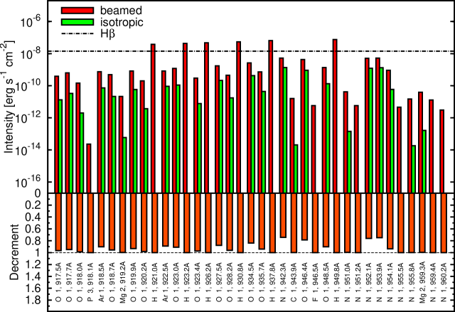
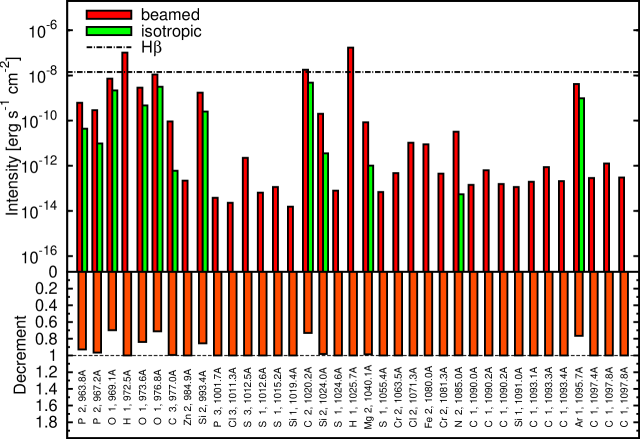
Figure 2.— Lines affected by the irradiation geometry from the ultraviolet to the infrared. (Top panel) Intensity obtained by not correcting for the incident continuum, “beamed” case, and by applying the corrections discussed in §6, “isotropic” case. The dot-dashed line indicates the H$\beta$ intensity computed for our model. (Bottom panel) Decremental change, defined as $\delta=1-I_{\mathrm{iso}}/I_{\mathrm{beam}}$, such that if the line intensity goes to zero after the continuum correction is applied, the decrement is 1. The species and wavelength of the transition is shown for each set of bars by the vertical labels at the bottom of the panel.

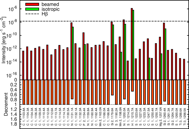
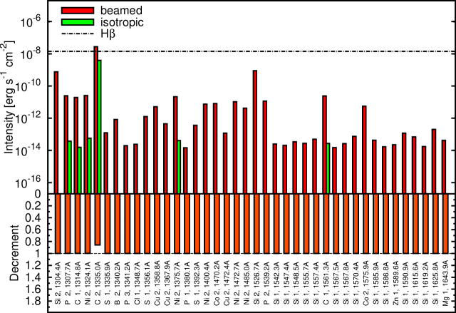
Figure 2.— (continued)

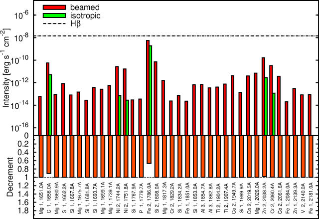
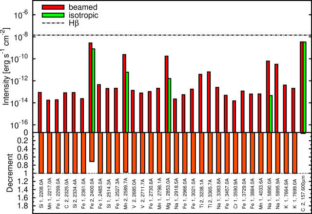
Figure 2.— (continued)

8. Conclusions

We have derived the escape probability theorem in the presence of external isotropic radiation, and we have shown that this effectively leads to a reduction of the net line emissivity relative to the unforced case. In essence then, the present theorem provides a means for a straightforward continuum subtraction for emission lines.

We have used our implementation of the theorem in Cloudy C13 to study the emission lines that arise from a typical Spitzer cloud in the presence of an external radiation field. We have found that about 60 percent of the emission lines are photo-excited and most of them susceptible to external field isotropy. In light of this finding, we argue that this mechanism may provide an additional tool toward quantifying the contributions of the isotropic starburst radiation field and the beamed AGN continuum in starburst galaxies and ULIRGs. A detailed study of the potential offered by this method is left for a future paper.

Appendix A A. Alternate Derivation of Irons’ Volume Average

The relation between averages of the net radiative bracket and the escape probability for some volume of the medium may also be obtained with the energy conservation arguments of Irons (1978).

Taking the emission-weighted average of equation (24) over volume, we obtain

$$\langle\rho\rangle_{V} = \frac{\int dV\,j(\mbox{\boldmath$r$})\,\rho(\mbox{\boldmath$r$})}{\int dV\,j(\mbox{\boldmath$r$})}$$ (A1)

$$= \frac{\int dV\,j(\mbox{\boldmath$r$})\,P_{e}(\mbox{\boldmath$r$})\,(1-J^{\mathrm{ext}}/S(\mbox{\boldmath$r$}))}{\int dV\,j(\mbox{\boldmath$r$})}$$

$$= \Bigl{\langle}P_{e}(\mbox{\boldmath$r$})\,\Bigl{(}1-\frac{J^{\mathrm{ext}}}{S(\mbox{\boldmath$r$})}\Bigr{)}\Bigr{\rangle}_{V}\,;$$

that is, we recover the same result as with Rybicki’s ray-based approach.

Appendix B B. Minimal Script for Astrophysical Application

The following script may be used to obtain the results presented in Figure 2.

ΨΨΨtitle cloud irradiated by ism background
ΨΨΨ#######################
ΨΨΨ# Set Continuum
ΨΨΨ#######################
ΨΨΨtable ism
ΨΨΨilluminate isotropic
ΨΨΨextinguish by a column of 22
ΨΨΨcosmic rays, background
ΨΨΨ#######################
ΨΨΨ# Set density & abundances
ΨΨΨ#######################
ΨΨΨhden 0
ΨΨΨatom chianti "CloudyChianti.ini"
ΨΨΨabundances ism
ΨΨΨ#######################
ΨΨΨ# Set Geometry
ΨΨΨ#######################
ΨΨΨsphere
ΨΨΨstop temperature linear 10
ΨΨΨstop thickness 0.1 linear parsecs
ΨΨΨ#######################
ΨΨΨ# Other details
ΨΨΨ#######################
ΨΨΨiterate to convergence
ΨΨΨ#Ψno lines continuum subtraction
ΨΨΨ#######################
ΨΨΨ# Output
ΨΨΨ#######################
ΨΨΨprint last
ΨΨΨprint line column
ΨΨΨprint line faint -6
ΨΨ

Appendix C C. Spectral Energy Distributions in Cloudy C13

Cloudy C13 includes a number of commands for generating radiation fields, as outlined below.

C.1. Isotropic Continua

table SED “cool.sed”
A cooling flow model based on Johnstone et al. (1992).

table draine
The galactic background radiation according to Draine & Bertoldi (1996), appropriate for simple photon-dominated region (PDR) simulations.

table hm96
The background continuum radiation at $z=2.16$ of Haardt & Madau (1996). It does not include the CMB.

table hm05
The radiation field of Haardt & Madau (2005, private communication with GJF) for any redshift out to $z=8.9$. It does not include the CMB.

table ism
The local interstellar radiation field of Black (1987).

table stars
External isotropic stellar continua, such as the output of Starburst99 (Leitherer et al., 1999).

C.2. Beamed Continua

table SED “akn120.sed”
An AGN continuum according to Peterson (private communication with GJF).

table SED “crab08.sed”/“crabdavidson.sed”
The continuum of the Crab Nebula, including the pulsar. The “crab08.sed” option utilizes the continuum of Atoyan & Aharonian (1996), while “crabdavidson.sed” enables the continuum of Davidson & Fesen (1985). The two differ significantly in the ultraviolet part of the spectrum.

table SED “rubin.sed”
Stellar spectrum that best matches the ionizing continuum of the Trapezium stars that illuminate the Orion Nebula. This is essentially a Kurucz (1979) stellar spectrum modified by R.H. Rubin.

table SED “xdr.sed”
Continuum of an X-ray dominated region (XDR) according to Maloney et al. (1996) in the range 1–100 keV.

table agn
Continuum appropriate for radio-quiet AGN, similar to Mathews & Ferland (1987), except for a break at 10 $\mu$m. At longer wavelengths the continuum of self-absorbed synchrotron radiation is used.

table power law
Power-law continuum appropriate for self-absorbed synchrotron radiation at low energies. At high energies the flux varies as $f_{\nu}\propto\nu^{-2}$. The extent of the mid-range and the spectral index therein are adjustable.

table stars
An extensive number of stellar spectra are available.

References

- Athay (1972) Athay, R. G. 1972, Radiation Transport in Spectral Lines (D. Reidel Publishing Company)
- Atoyan & Aharonian (1996) Atoyan, A. M., & Aharonian, F. A. 1996, MNRAS, 278, 525
- Black (1987) Black, J. H. 1987, in Astrophysics and Space Science Library, Vol. 134, Interstellar Processes, ed. D. J. Hollenbach & H. A. Thronson, Jr., 731–744
- Castor (1970) Castor, J. I. 1970, MNRAS, 149, 111
- Cowie & Songaila (1986) Cowie, L. L., & Songaila, A. 1986, ARA&A, 24, 499
- Dalgarno et al. (1999) Dalgarno, A., Yan, M., & Liu, W. 1999, ApJS, 125, 237
- Davidson & Fesen (1985) Davidson, K., & Fesen, R. A. 1985, ARA&A, 23, 119
- D’Cruz et al. (1998) D’Cruz, N. L., Sarazin, C. L., & Dubau, J. 1998, ApJ, 501, 414
- Dere et al. (1997) Dere, K. P., Landi, E., Mason, H. E., Monsignori Fossi, B. C., & Young, P. R. 1997, A&AS, 125, 149
- Draine & Bertoldi (1996) Draine, B. T., & Bertoldi, F. 1996, ApJ, 468, 269
- Elitzur (1984) Elitzur, M. 1984, ApJ, 280, 653
- Elitzur (1992) Elitzur, M., ed. 1992, Astrophysics and Space Science Library, Vol. 170, Astronomical masers
- Ferland et al. (2013) Ferland, G. J., Porter, R. L., van Hoof, P. A. M., et al. 2013, Revista Mexicana de Astronomia y Astrofisica, 49, 137
- Genzel & Cesarsky (2000) Genzel, R., & Cesarsky, C. J. 2000, ARA&A, 38, 761
- Goldreich & Kwan (1974) Goldreich, P., & Kwan, J. 1974, ApJ, 189, 441
- Haardt & Madau (1996) Haardt, F., & Madau, P. 1996, ApJ, 461, 20
- Irons (1978) Irons, F. E. 1978, MNRAS, 182, 705
- Jefferies (1968) Jefferies, J. T. 1968, Spectral line formation (Blaisdell Publishing Company)
- Johnstone et al. (1992) Johnstone, R. M., Fabian, A. C., Edge, A. C., & Thomas, P. A. 1992, MNRAS, 255, 431
- Kurucz (1979) Kurucz, R. L. 1979, ApJS, 40, 1
- Landi et al. (2012) Landi, E., Del Zanna, G., Young, P. R., Dere, K. P., & Mason, H. E. 2012, ApJ, 744, 99
- Leitherer et al. (1999) Leitherer, C., Schaerer, D., Goldader, J. D., et al. 1999, ApJS, 123, 3
- Maloney et al. (1996) Maloney, P. R., Hollenbach, D. J., & Tielens, A. G. G. M. 1996, ApJ, 466, 561
- Mathews & Ferland (1987) Mathews, W. G., & Ferland, G. J. 1987, ApJ, 323, 456
- Mathis et al. (1977) Mathis, J. S., Rumpl, W., & Nordsieck, K. H. 1977, ApJ, 217, 425
- Meyer et al. (1998) Meyer, D. M., Jura, M., & Cardelli, J. A. 1998, ApJ, 493, 222
- Mullman et al. (1998) Mullman, K. L., Lawler, J. E., Zsargo, J., & Federman, S. R. 1998, ApJ, 500, 1064
- Osterbrock (1962) Osterbrock, D. E. 1962, ApJ, 135, 195
- Rybicki (1984) Rybicki, G. B. 1984, in Methods in Radiative Transfer, ed. W. Kalkofen (Cambridge University Press), 21–64
- Savage & Sembach (1996) Savage, B. D., & Sembach, K. R. 1996, ARA&A, 34, 279
- Schöier et al. (2005) Schöier, F. L., van der Tak, F. F. S., van Dishoeck, E. F., & Black, J. H. 2005, A&A, 432, 369
- Snow et al. (2007) Snow, T. P., Destree, J. D., & Jensen, A. G. 2007, ApJ, 655, 285
- Spitzer (1978) Spitzer, L. 1978, Physical processes in the interstellar medium (New York Wiley-Interscience), 333 p.
- Sunyaev & Docenko (2007) Sunyaev, R. A., & Docenko, D. O. 2007, Astronomy Letters, 33, 67