Spectrum of excited states using the stochastic LapH method

Abstract:

Progress in computing the spectrum of excited baryons and mesons in lattice QCD is described. Our first results in the zero-momentum bosonic $I=1,\ S=0,\ T_{1u}^{+}$ symmetry sector of QCD using a correlation matrix of 56 operators are presented. In addition to a dozen spatially-extended meson operators, 44 two-meson operators are used, involving a wide variety of light isovector, isoscalar, and strange meson operators of varying relative momenta. All needed Wick contractions are efficiently evaluated using a stochastic method of treating the low-lying modes of quark propagation that exploits Laplacian Heaviside quark-field smearing. Level identification is discussed.

1 Introduction

In a series of papers[1, 2, 3, 4, 5, 6, 7], we have been striving to compute the finite-volume stationary-state energies of QCD using Markov-chain Monte Carlo integration of the QCD path integrals formulated on a space-time lattice. In this talk and accompanying poster, our progress towards this goal is described. We present our first results in the zero-momentum bosonic $I=1,\ S=0,\ T_{1u}^{+}$ symmetry sector of QCD using a correlation matrix of 56 operators. In addition to a dozen spatially-extended meson operators, an unprecedented number of 44 two-meson operators are used, involving a wide variety of light isovector, isoscalar, and strange meson operators of varying relative momenta. All needed Wick contractions are efficiently evaluated using a stochastic method of treating the low-lying modes of quark propagation that exploits Laplacian Heaviside quark-field smearing. Given the large number of levels extracted, level identification becomes a key issue.

This paper is organized as follows. The single-hadron and two-hadron operators that we use are briefly reviewed in Sec. 2. Our method of extracting the energies and overlaps is described in Sec. 3. First-pass results are then presented in Sec. 4, and the issue of level identification is confronted. Concluding remarks are given in Sec. 5.

2 Single-hadron and multi-hadron operators

The stationary-state energies in a particular symmetry sector can be extracted from an $N\times N$ Hermitian correlation matrix ${\cal C}_{ij}(t)=\langle 0|\,O_{i}(t\!+\!t_{0})\,\overline{O}_{j}(t_{0})\ |0\rangle,$ where the $N$ operators $\overline{O}_{j}$ act on the vacuum to create the states of interest at source time $t_{0}$ and are accompanied by conjugate operators $O_{i}$ that can annihilate these states at a later time $t+t_{0}$. Estimates of ${\cal C}_{ij}(t)$ are obtained with the Monte Carlo method using the stochastic LapH method[6] which allows all needed quark-line diagrams to be computed. The operators that we use have been described in detail in Refs. [1, 6, 7], but a brief review of our operator design is presented below.

Our hadron operators are constructed using spatially smoothened link variables $\widetilde{U}_{j}(x)$ and spatially smeared quark fields $\widetilde{\psi}(x)$. The spatial links are smeared using the stout-link procedure described in Ref. [8]. The smeared quark field for each quark flavor is defined by

$$\widetilde{\psi}_{a\alpha}(x)={\cal S}_{ab}(x,y)\ \psi_{b\alpha}(y),$$ (1)

where $x,y$ are lattice sites, $a,b$ are color indices, and $\alpha$ is a Dirac spin component. We use the Laplacian Heaviside (LapH) quark-field smearing scheme introduced in Ref. [9] and defined by

$${\cal S}=\Theta\left(\sigma_{s}^{2}+\widetilde{\Delta}\right),$$ (2)

where $\widetilde{\Delta}$ is the three-dimensional gauge-covariant Laplacian defined in terms of the stout-smeared gauge field $\widetilde{U}$, and $\sigma_{s}$ is the smearing cutoff parameter. More details concerning this smearing scheme are described in Ref. [6].

All of our single-hadron operators are assemblages of basic building blocks which are gauge-covariantly-displaced, LapH-smeared quark fields:

$$q^{A}_{a\alpha j}=D^{(j)}\widetilde{\psi}_{a\alpha}^{(A)},\qquad\overline{q}^{A}_{a\alpha j}=\widetilde{\overline{\psi}}_{a\alpha}^{(A)}\gamma_{4}\,D^{(j)\dagger},$$ (3)

where $a$ is a color index, $\alpha$ is a Dirac spin component, $A$ is a quark flavor, $\gamma_{4}$ is the temporal Dirac $\gamma$-matrix, and the displacement $D^{(j)}$ is a product of smeared link variables:

$$D^{(j)}(x,x^{\prime})=\widetilde{U}_{j_{1}}(x)\ \widetilde{U}_{j_{2}}(x\!+\!d_{2})\ \widetilde{U}_{j_{3}}(x\!+\!d_{3})\dots\widetilde{U}_{j_{p}}(x\!+\!d_{p})\delta_{x^{\prime},x+d_{p+1}}.$$ (4)

The use of $\gamma_{4}$ in Eq. (3) is convenient for obtaining baryon correlation matrices that are Hermitian.

We can simplify our spectrum calculations as much as possible by working with single-hadron operators that transform irreducibly under all symmetries of a three-dimensional cubic lattice of infinite extent or finite extent with periodic boundary conditions. The construction of irreducible representations (irreps) of $O_{h}^{1}$ begins with the irreps of the abelian subgroup of lattice translations. These are characterized by a definite three-momentum $\bm{p}$ as allowed by the periodic boundary conditions. Each of our meson and baryon operators which creates a three-momentum $\bm{p}$ is a linear superposition of gauge-invariant quark-antiquark and three-quark elemental operators of the form

$$\overline{\Phi}_{\alpha\beta}^{AB}(\bm{p},t) = \sum_{\bm{x}}e^{i\bm{p}\cdot(\bm{x}+\frac{1}{2}(\bm{d}_{\alpha}+\bm{d}_{\beta}))}\delta_{ab}\ \overline{q}^{B}_{b\beta}(\bm{x},t)\ q^{A}_{a\alpha}(\bm{x},t),$$ (5)

$$\overline{\Phi}_{\alpha\beta\gamma}^{ABC}(\bm{p},t) = \sum_{\bm{x}}e^{i\bm{p}\cdot\bm{x}}\varepsilon_{abc}\ \overline{q}^{C}_{c\gamma}(\bm{x},t)\ \overline{q}^{B}_{b\beta}(\bm{x},t)\ \overline{q}^{A}_{a\alpha}(\bm{x},t),$$ (6)

where $q,\overline{q}$ are defined in Eq. (3), $\bm{d}_{\alpha},\bm{d}_{\beta}$ are the spatial displacements of the $\overline{q},q$ fields, respectively, from $\bm{x}$, $A,B$ indicate flavor, and $\alpha,\beta$ are compound indices incorporating both spin and quark-displacement types. The phase factor involving the quark-antiquark displacements is needed to ensure proper transformation properties under $G$-parity for arbitrary displacement types. Group theory projections onto the irreps of the lattice symmetry group are then employed. Each meson and baryon source operator ends up having the form

$$\overline{M}_{l}(t)=c_{\alpha\beta}^{(l)\ast}\ \overline{\Phi}_{\alpha\beta}^{AB}(t),\qquad\overline{B}_{l}(t)=c_{\alpha\beta\gamma}^{(l)\ast}\ \overline{\Phi}_{\alpha\beta\gamma}^{ABC}(t),$$ (7)

(or is a flavor combination of the above form), where $l$ is a compound index comprised of a three-momentum $\bm{p}$, an irreducible representation $\Lambda$ of the little group of $\bm{p}$, the row $\lambda$ of the irrep, total isospin $I$, isospin projection $I_{3}$, strangeness $S$, and an identifier labeling the different operators in each symmetry channel. Here, we focus on mesons containing only $u,d,s$ quarks. In order to build up the necessary orbital and radial structures expected in the hadron excitations, we use a variety of spatially-extended configurations for our hadron operators, as shown in Table 1.

Table 1: The spatial arrangements of the quark-antiquark meson operators and the three-quark baryon operators. In the illustrations, the smeared quarks fields are depicted by solid circles, each hollow circle indicates a smeared “barred” antiquark field, the solid line segments indicate covariant displacements, and each hollow box indicates the location of a Levi-Civita color coupling. For simplicity, all displacements have the same length in an operator.

We construct our two-hadron operators as superpositions of single-hadron operators of definite momenta. Each single-hadron operator is labelled by total isospin $I$, the projection of the total isospin $I_{3}$, strangeness $S$, three-momentum $\bm{p}$, the little group irrep $\Lambda$, the row of the irrep $\lambda$, and $i$, which denotes all other identifying information, such as the displacement type and index. Hence, the two-hadron operators have the form

$$c^{I_{3a}I_{3b}}_{\bm{p}_{a}\lambda_{a};\ \bm{p}_{b}\lambda_{b}}\ B^{I_{a}I_{3a}S_{a}}_{\bm{p}_{a}\Lambda_{a}\lambda_{a}i_{a}}\ B^{I_{b}I_{3b}S_{b}}_{\bm{p}_{b}\Lambda_{b}\lambda_{b}i_{b}},$$ (8)

for fixed total momentum $\bm{p}=\bm{p}_{a}+\bm{p}_{b}$, and fixed $\Lambda_{a},i_{a},\Lambda_{b},i_{b}$. Once again, group theory projections onto the little group of $\bm{p}$ and the isospin irreps are carried out. For practical reasons, we restrict our attention to certain classes of momentum directions for the single hadron operators: on axis $\pm\widehat{\bm{x}},\ \pm\widehat{\bm{y}},\ \pm\widehat{\bm{z}}$, planar diagonal $\pm\widehat{\bm{x}}\pm\widehat{\bm{y}},\ \pm\widehat{\bm{x}}\pm\widehat{\bm{z}},\ \pm\widehat{\bm{y}}\pm\widehat{\bm{z}}$, and cubic diagonal $\pm\widehat{\bm{x}}\pm\widehat{\bm{y}}\pm\widehat{\bm{z}}$. It is crucial to know and fix all phases of the single-hadron operators for all momenta. To do this, we choose a reference direction $\bm{p}_{\rm ref}$ for each class of momentum directions, and for each $\bm{p}$, we select one reference rotation $R_{\rm ref}^{\bm{p}}$ that transforms $\bm{p}_{\rm ref}$ into $\bm{p}$. The details are described in Ref. [7]. This approach is efficient for creating large numbers of two-hadron operators, and generalizes to three or more hadrons.

In addition to efficiency, there are good physical reasons for using such multi-hadron operators. Hadron-hadron interactions in finite volume move the energies of any two-hadron systems away from their free two-particle energies, and the interacting two-particle states could involve distributions of different relative momenta. However, such interactions are usually small and the relative momenta used in our operators should presumably dominate in most cases. Also, we will always utilize multi-hadron operators with a variety of different relative momenta to accommodate the effects of such interactions. The performance of some of our $\pi\pi$ operators are compared to localized multi-hadron operators in Fig. 1, discussed below.

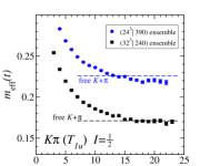
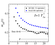
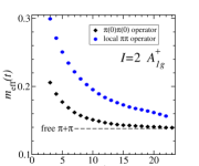
Figure 1: (Left) Effective masses, $m_{\rm eff}(t)$, associated with a two-meson operator in the $T_{1u}$ irrep, having total isospin $I=\frac{1}{2}$ and zero total momentum, constructed from single-site kaon and pion operators having equal and opposite on-axis momenta of minimal nonzero magnitude. Results on the $(24^{3}|390)$ and $(32^{3}|240)$ ensembles (see text) are shown. The energies of a free $\pi$ plus a free $K$ are indicated by horizontal dashed lines. (Center) Effective mass for one of our $I=1$ $\pi(1)\pi(-1)$ operators in the $T_{1u}^{+}$ channel, consisting of single-site pion operators having equal and opposite on-axis momenta of minimal nonzero magnitude, compared to the effective mass of a localized $\pi\pi$ operator, described in Eq. (10), on the $(24^{3}|390)$ ensemble. (Right) Effective mass for one of our $I=2$ $\pi(0)\pi(0)$ operators in the $A_{1g}^{+}$ channel, consisting of single-site pion operators each having zero momenta, compared to the effective mass of a localized $\pi\pi$ operator, described in Eq. (9), on the $(24^{3}|390)$ ensemble.

In order to test the effectiveness of the two-hadron operators that we have designed, we examined the effective masses associated with the correlators of a variety of two-hadron operators. In the left plot of Fig. 1, effective masses associated with a two-meson operator in the $T_{1u}$ irrep are shown. The two-meson operator has total isospin $I=\frac{1}{2}$ and zero total momentum and is constructed from single-site kaon and pion operators having equal and opposite on-axis momenta of minimal nonzero magnitude. Results on the $(24^{3}|390)$ and $(32^{3}|240)$ ensembles (described below) are shown and compared to the energies of a free $\pi$ plus a free $K$, indicated by horizontal dashed lines.

An alternative design for a two-hadron operator is to use a suitable localized-field operator. For example, localized $\pi\pi$ operators in the $I=2,\ A_{1g}^{+}$ and $I=1,\ T_{1u}^{+}$ channels can be obtained using

$$(\pi\pi)^{A_{1g}^{+}}(t) = \sum_{\bm{x}}\pi^{+}(\bm{x},t)\ \pi^{+}(\bm{x},t),$$ (9)

$$(\pi\pi)^{T_{1u}^{+}}(t) = \!\!\!\!\!\sum_{\bm{x},k=1,2,3}\!\!\!\!\Bigl{\{}\pi^{+}(\bm{x},t)\ \Delta_{k}\pi^{0}(\bm{x},t)-\pi^{0}(\bm{x},t)\ \Delta_{k}\pi^{+}(\bm{x},t)\Bigr{\}},$$ (10)

where $\pi(\bm{x},t)$ is a single-site pion field using a standard $\gamma_{5}$ construction with the LapH-smeared quark fields, and $\Delta_{k}\pi(\bm{x},t)=\pi(\bm{x}\!+\!\widehat{\bm{k}},t)-\pi(\bm{x}\!-\!\widehat{\bm{k}},t)$. The superscripts indicate the electric charges associated with each field. In such localized $\pi\pi$ operators, the individual pions do not have definite momenta.

The center and right plots of Fig. 1 compare the effective masses for our $\pi\pi$ operators to those for these localized $\pi\pi$ operators. The center plot of Fig. 1 shows the effective mass for one of our $I=1$ $\pi(1)\pi(-1)$ operators in the $T_{1u}^{+}$ channel, consisting of single-site pion operators having equal and opposite on-axis momenta of minimal nonzero magnitude, compared to the effective mass of the localized $\pi\pi$ operator, given in Eq. (10), on the $(24^{3}|390)$ ensemble. The right plot of Fig. 1 shows the effective mass for one of our $I=2$ $\pi(0)\pi(0)$ operators in the $A_{1g}^{+}$ channel, consisting of single-site pion operators each having zero momenta, compared to the effective mass of the localized $\pi\pi$ operator, given in Eq. (9), on the $(24^{3}|390)$ ensemble. One sees that the effective masses of the localized $\pi\pi$ operators lie well above those of our operators, indicating that they contain much more excited-state contamination. These effective masses are compared to the energies of the ground state $\rho$ and the free $\pi+\pi$ energies, indicated by horizontal dashed lines, in this figure. Note that, in addition to having much less excited-state contamination, the two-pion operators comprised of individual pions having definite momenta are also much easier to make in large numbers, compared to the localized multi-hadron operators.

3 Energy and overlap extractions

For the large numbers of operators we plan to use, it can happen that the condition number of the correlation matrix can grow uncomfortably large. In a large matrix of correlations, statistical noise can cause the matrix to become ill-conditioned, or even to have negative eigenvalues so that the matrix is no longer positive definite. It is important to monitor this and take corrective actions. We do this as follows. Starting with a raw correlation matrix ${\cal C}(t)$, we first try to remove the effects of differing normalizations by forming the matrix $\widehat{C}_{ij}(t)={\cal C}_{ij}(t)\ (\ {\cal C}_{ii}(\tau_{N}){\cal C}_{jj}(\tau_{N})\ )^{-1/2}$, taking $\tau_{N}$ at a very early time, such as $\tau_{N}=3$. We then pick a large value $t=t_{F}$ and evaluate the eigenvalues and eigenvectors of $\widehat{C}(t_{F})$. Since the matrix is Hermitian, the eigenvalues are real and the eigenvectors are orthonormal. Let $U_{N}$ denote the unitary matrix whose columns are the eigenvectors of $\widehat{C}(t_{F})$. The columns corresponding to negative eigenvalues must be removed. We also remove the columns corresponding to eigenvalues that are positive, but small. In other words, we remove the columns from $U_{N}$ for all eigenvalues less than some threshold $\lambda_{\rm threshold}$. Let $P_{N}$ denote the projection matrix whose columns are the retained columns (eigenstates) of $U_{N}$. We then apply this projection to the correlators to obtain a new correlation matrix $C(t)$:

$$C(t)=P_{N}^{\dagger}\ \widehat{C}(t)\ P_{N}.$$ (11)

The threshold $\lambda_{\rm threshold}$ is determined as follows. We decide on the largest value of the condition number that is acceptable, denoting this by $\xi^{\rm cn}_{\rm max}$. We determine the largest eigenvalue $\lambda_{\rm max}$, then since the condition number is the ratio of the largest eigenvalue over the eigenvalue of smallest magnitude, the minimum allowed eigenvalue is

$$\lambda_{\rm threshold}=\frac{\lambda_{\rm max}}{\xi^{\rm cn}_{\rm max}}.$$ (12)

The above procedure ensures that $C(t_{F})$ is positive-definite and well conditioned. We also check this for all other $t$ values that we use. Extraction of the energies then proceeds using the refined correlator $C(t)$.

In finite volume, all energies are discrete so that each correlator matrix element has a spectral representation of the form

$$C_{ij}(t)=\sum_{n}Z_{i}^{(n)}Z_{j}^{(n)\ast}\ e^{-E_{n}t},\qquad\quad Z_{j}^{(n)}=\langle 0|\ O_{j}\ |n\rangle,$$ (13)

assuming temporal wrap-around (thermal) effects are negligible. For temporal separations $t$ large enough such that only the lowest $N$ energies contribute, we can solve for $E_{n}$ and $Z_{j}^{(n)}$ using the correlation matrix at two time separations $C(\tau_{0})$ and $C(t)$. We first solve the generalized eigenvector problem $Ax=\lambda Bx$ with $A=C(t)$ and $B=C(\tau_{0})$. We put the eigenvectors into the columns of the matrix $V$ with normalization condition $V^{\dagger}C(\tau_{0})V=I$, and the eigenvalue corresponding to column $n$ is $\lambda_{n}=e^{-E_{n}(t-\tau_{0})}$. Then the overlaps are given by

$$Z_{j}^{(n)}=C_{jk}(\tau_{0})\ V_{kn}\ e^{E_{n}\tau_{0}/2}.$$

If $\tau_{0}$ and $t$ are chosen such that the contributions to all $C_{ij}(\tau_{0})$ and $C_{ij}(t)$ from all levels above the lowest $N$ energies are negligible, then the results obtained for the $E_{n}$ and $Z_{j}^{(n)}$ will be the same for all suitably large $\tau_{0}$ and $t$. To check this, one usually fixes $\tau_{0}$ and varies $t$, making $t$ larger and larger until the solved values for $E_{n}$ and $Z_{j}^{(n)}$ become independent of $t$.

For fixed $\tau_{0}$ (which must be suitably large), these solutions for $E_{n}$ and $Z_{j}^{(n)}$ can be viewed as functions of $t$, and one can even perform fits to these functions with simple empirically-motivated forms to extract their large $t$ values. For example, the $N$ eigenvalues of $C(\tau_{0})^{-1/2}\ C(t)\ C(\tau_{0})^{-1/2}$ are known as the principal correlators and are denoted by $\lambda_{\alpha}(t,\tau_{0})$. As $t$ becomes large,

$$\lim_{t\rightarrow\infty}\lambda_{\alpha}(t,\tau_{0})=e^{-(t-\tau_{0})E_{\alpha}}.$$ (14)

This already complicated procedure is further plagued by the issue of eigenvector identification. Eigenvector “pinning” is usually needed in this method to deal with level switching. Since the eigenvalue equation is solved for eigenvalues $E_{n}$ and eigenvectors $v^{(n)}$, independently on each timeslice $t$ and for each bootstrap sample, ensuring the same ordering of states between time slices and bootstrap samples requires some care, especially when levels are closely spaced or nearly degenerate. Instead of ordering by the value of the eigenvalue, one associates states between neighboring time slices and bootstrap samples using the similarity of their eigenvectors. For ordering the states on time $t$ using the full ensemble, one uses the eigenvectors obtained on the full ensemble (not a bootstrap sample) on timeslice $t-1$ as the reference eigenvectors $v^{(n)}_{\rm ref}$. The eigenvector comparison is done by finding the maximum value of $v^{(n^{\prime})\dagger}_{\rm ref}C(\tau_{0})v^{(n)}$ which associates a state $n$ with a reference state $n^{\prime}$. When ordering levels in a bootstrap sample for time $t$, one uses the eigenvectors obtained on the full ensemble for time $t$ as the references.

The above “principal correlator method” is rather costly and complicated. Diagonalizations must be carried out for a large number of times $t$, and the diagonalizations at large times can amplify errors and possibly introduce bias. Also, the eigenvector “pinning” is somewhat ad hoc, and hence, unpalatable. A simpler method, which here is called the “single rotation” method, or the “fixed coefficient” method, performs the diagonalization with one choice of metric time $\tau_{0}$ and one time $t=\tau_{D}$. The eigenvectors obtained are used to “rotate” the original correlator $C(t)$ into a correlator $G(t)$ for which $G(\tau_{0})=1$, the identity matrix, and $G(\tau_{D})$ is diagonal. At other times, $G(t)$ need not be diagonal. However, with judicious choices of $\tau_{0}$ and $\tau_{D}$, one finds that the off-diagonal elements of $G(t)$ remain zero within statistical precision for $t>\tau_{D}$. The rotated correlator is given by

$$G(t)=U^{\dagger}\ C(\tau_{0})^{-1/2}\ C(t)\ C(\tau_{0})^{-1/2}\ U,$$ (15)

where the columns of $U$ are the orthonormalized eigenvectors of $C(\tau_{0})^{-1/2}\ C(\tau_{D})\ C(\tau_{0})^{-1/2}$. Rotated effective masses can then be defined by

$$m_{G}^{(n)}(t)=\frac{1}{\Delta t}\ln\left(\frac{G_{nn}(t)}{G_{nn}(t+\Delta t)}\right),$$ (16)

which tend to the lowest-lying $N$ stationary-state energies produced by the $N$ operators. Correlated-$\chi^{2}$ fits to the estimates of $G_{nn}(t)$ using the forms $A_{n}(e^{-E_{n}\,t}+e^{-E_{n}\,(T-t)})$, where $T$ is the temporal extent of the lattice, yield the energies $E_{n}$ and the overlaps $A_{n}$ to the rotated operators for each $n$. Using the rotation coefficients, one can then easily obtain the overlaps $Z^{(n)}_{j}=C(\tau_{0})^{1/2}_{jk}\ U_{kn}\ A_{n}$ (no summation over $n$) corresponding to the rows and columns of the correlation matrix $C(t)$. Use of the $P_{N}$ matrix gives the overlaps for the original operator set, modulo a normalization factor for each operator.

4 First results

We are currently focusing on three Monte Carlo ensembles: (A) a set of 412 gauge-field configurations on a large $32^{3}\times 256$ anisotropic lattice with a pion mass $m_{\pi}\sim 240$ MeV, (B) an ensemble of 551 configurations on an $24^{3}\times 128$ anisotropic lattice with a pion mass $m_{\pi}\sim 390$ MeV, and (C) an ensemble of 584 configurations on an $24^{3}\times 128$ anisotropic lattice with a pion mass $m_{\pi}\sim 240$ MeV. We refer to these ensembles as the $(32^{3}|240)$, $(24^{3}|390)$, and $(24^{3}|240)$ ensembles, respectively. These ensembles were generated using the Rational Hybrid Monte Carlo (RHMC) algorithm[10]. In each ensemble, successive configurations are separated by 20 RHMC trajectories to minimize autocorrelations. An improved anisotropic clover fermion action and an improved gauge field action are used[11]. In these ensembles, $\beta=1.5$ and the $s$ quark mass parameter is set to $m_{s}=-0.0743$ in order to reproduce a specific combination of hadron masses[11]. In the $(24^{3}|390)$ ensemble, the light quark mass parameters are set to $m_{u}=m_{d}=-0.0840$ so that the pion mass is around 390 MeV if one sets the scale using the $\Omega$ baryon mass. In the $(32^{3}|240)$ and $(24^{3}|240)$ ensembles, $m_{u}=m_{d}=-0.0860$ are used, resulting in a pion mass around 240 MeV. The spatial grid size is $a_{s}\sim 0.12$ fm, whereas the temporal spacing is $a_{t}\sim 0.035$ fm.

In our operators, a stout-link staple weight $\xi=0.10$ is used with $n_{\xi}=10$ iterations. For the cutoff in the LapH smearing, we use $\sigma_{s}^{2}=0.33$, which translates into the number $N_{v}$ of LapH eigenvectors retained being $N_{v}=112$ for the $24^{3}$ lattices and $N_{v}=264$ for the $32^{3}$ lattice. We use $Z_{4}$ noise in all of our stochastic estimates of quark propagation. Our variance reduction procedure is described in Ref. [6]. On the $24^{3}$ lattices, we use 4 widely-separated source times $t_{0}$, and 8 are used on the $32^{3}$ lattice.

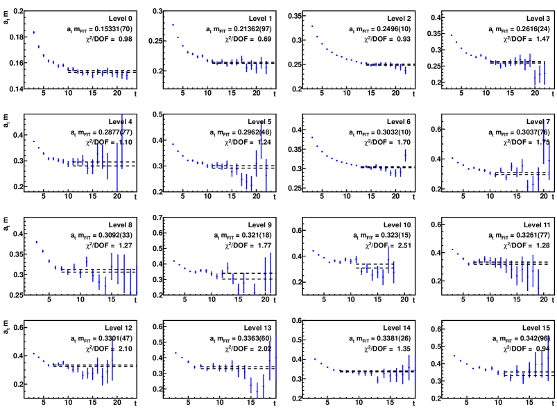
Figure 2: Rotated effective masses $m_{G}^{(n)}(t)$ (see Eq. (16)) for the 16 lowest-lying energy levels in the zero-momentum bosonic $I=1,\ S=0,\ T_{1u}^{+}$ channel for the $(24^{3}|390)$ ensemble using 12 single-meson operators, 17 isovector+isovector operators, 17 isoscalar+isovector operators, and 10 kaon+antikaon operators. Dashed lines indicate energy extractions from correlated-$\chi^{2}$ fits. Fit results and qualitites are also listed in each plot.

The Monte Carlo method commonly employed in QCD computations applies only to space-time lattices of finite extent. Hence, the energies we extract are those associated with the stationary states of QCD in a cubic box using periodic boundary conditions. In such a cubic box, we no longer have full rotational symmetry, even in the continuous space-time limit. The stationary states cannot be labelled by the usual spin-$J$ quantum numbers. Instead, the stationary states in a box with periodic boundary conditions must be labelled by the irreducible representations (irreps) of the cubic space group, even in the continuum limit. A detailed description of these irreps is summarized in Ref. [7].

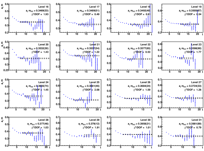
Figure 3: Rotated effective masses $m_{G}^{(n)}(t)$ (see Eq. (16)) for energy levels 16 to 31 in the zero-momentum bosonic $I=1,\ S=0,\ T_{1u}^{+}$ channel for the $(24^{3}|390)$ ensemble using 12 single-meson operators, 17 isovector+isovector operators, 17 isoscalar+isovector operators, and 10 kaon+antikaon operators. Dashed lines indicate energy extractions from correlated-$\chi^{2}$ fits. Fit results and qualitites are also listed in each plot.

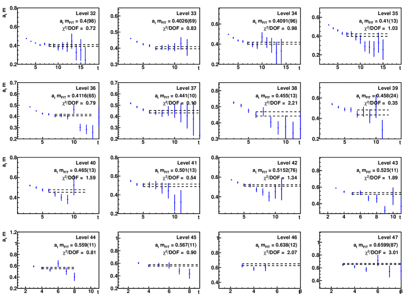
Figure 4: Rotated effective masses $m_{G}^{(n)}(t)$ (see Eq. (16)) for energy levels 32 to 47 in the zero-momentum bosonic $I=1,\ S=0,\ T_{1u}^{+}$ channel for the $(24^{3}|390)$ ensemble using 12 single-meson operators, 17 isovector+isovector operators, 17 isoscalar+isovector operators, and 10 kaon+antikaon operators. Dashed lines indicate energy extractions from correlated-$\chi^{2}$ fits. Fit results and qualitites are also listed in each plot.

For our first calculations, we decided to focus on the resonance-rich $I=1,\ S=0,\ T_{1u}^{+}$ channel of total zero momentum. This channel has odd parity, even $G$-parity, and contains the spin-1 and spin-3 mesons. The experimentally-known resonances in this channel include the $\rho(770)$, $\rho(1450)$, $\rho(1570),$ $\rho_{3}(1690),$ and $\rho(1700)$. Low statistics runs on smaller lattices led us to include 12 particular single-meson (quark-antiquark) operators. We took special care to include operators that could produce the spin-$3$ $\rho_{3}(1690)$ state, in addition to the other spin-$1$ states. Low statistics runs also gave us the masses of the lowest-lying mesons, such as the $\pi,\eta,K,$ and so on. Given these known mesons, we used software written in Maple to find all possible two-meson states in our cubic box in this $T_{1u}^{+}$ symmetry channel, assuming no energy shifts from interactions or the finite volume. We used these so-called “expected two-meson levels” to guide our choice of two-meson operators to include. We included 17 isovector-isovector meson operators, 14 operators that combine an isovector with a light isoscalar (using only $u,d$ quarks), 3 operators that combine an isovector with an $\overline{s}s$ isoscalar meson, and 10 kaon-antikaon operators. Our “first-pass” results for the $(24^{3}|390)$ ensemble obtained from our $56\times 56$ correlation matrix are presented in Figs. 2, 3, and 4. The rotated effective masses $m_{G}^{(n)}(t)$ (see Eq. (16)) using $\tau_{0}=5$ and $\tau_{D}=9$ are shown in these figures. Fits values and qualities are listed, and depicted by the horizontal dashed lines.

The results shown here are not finalized yet. We are still varying the fitting ranges to improve the $\chi^{2}$, as needed in some instances. We are investigating the effects of adding more operators, and we are even still verifying our analysis/fitting software. However, these figures do demonstrate that the extraction of a large number of energy levels is indeed possible, and the plots indicate the level of precision that can be attained with our stochastic LapH method. Keep in mind that we have not included any three-meson operators in our correlation matrix.

With such a large number of energies extracted, level identification becomes a key issue. QCD is a complicated interacting quantum field theory, so characterizing its stationary states in finite volume is not likely to be done in a simple way. Level identification must be inferred from the $Z$ overlaps of our probe operators, analogous to deducing resonance properties from scattering cross sections in experiments. Although we are in control of the probe operators $\overline{O}_{j}$ which act on the vacuum to create “probe states” $|\Phi_{j}\rangle\equiv\overline{O}_{j}|0\rangle$, we have limited knowledge and control of the probe states so produced. Judiciously chosen probe operators, constructed from smeared fields, should excite the low-lying states of interest, with hopefully little coupling to unwanted higher-lying states, and help with classifying the levels extracted. Small-$a$ classical expansions can help to characterize the probe operators, and hence, the states they produce.

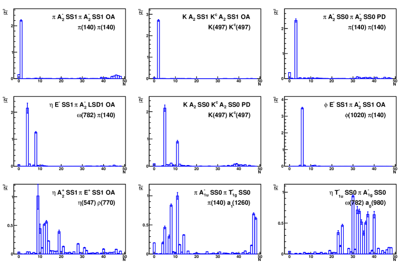
Figure 5: Overlaps $|Z^{(n)}_{j}|^{2}$ for some selected operators $O_{j}$ against the eigenstates labelled by $n$. The selected operators are listed in the top right corner of each plot, and the physical content of the dominant state for that operator is also listed. The overall normalization is arbitrary in each plot.

The overlaps $|Z^{(n)}_{j}|^{2}$ corresponding to some selected operators are shown in Fig. 5. In the first plot (upper left), one sees that this operator mainly creates level 1 (the first excited state in this channel). The overlaps onto all other states are very small. This operator is constructed from two pion operators, each having a well defined momentum of minimal magnitude along the lattice axes; the pions have equal and opposite momenta so that the total momentum is zero, and the momentum directions are combined so as to produce the $T_{1u}^{+}$ quantum numbers. Hence, we can identify level 1 as dominantly a two-pion state in which the pions have minimal relative momentum allowed for a $T_{1u}^{+}$ level. An operator expected to create a state dominated by the $\rho$ meson at rest mainly produces level 0 (not shown), but one sees that this two-pion operator does have some overlap onto the ground state. We infer that level 0 is dominated by the $\rho$ at rest, but does have a small admixture of two-pion states. The second plot shows that its operator mainly produces level 2 (the second excited state). This operator is expected to mainly create a kaon-antikaon state, so we identify this level as a low-lying kaon-antikaon state. For many levels, one finds that one or a handful of probe states dominate, making classification straightforward. However, Fig. 5 also shows cases where a given operator creates several eigenstates, making classification of some levels problematic.

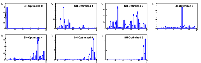
Figure 6: Overlaps $|\widetilde{Z}^{(n)}_{j}|^{2}$ of “optimized” single-hadron operator $\widetilde{O}_{j}$ against the eigenstates labelled by $n$. The overall normalization is arbitrary in each plot.

We will focus our efforts on level identification much more in our future work. For now, we mainly wish to identify the levels that dominate the finite-volume stationary states expected to evolve into the single-meson resonances in infinite volume. We view such states as “resonance precursor states”. To accomplish this, we utilize “optimized” single-hadron operators as our probes. We first restrict our attention to the $12\times 12$ correlator matrix involving only the 12 chosen single-hadron operators. We then perform an optimization rotation to produce so-called “optimized” single-hadron (SH) operators $\widetilde{O}_{j}$, which are linear combinations of the 12 original operators, determined in a manner analogous to Eq. (15). The effective masses corresponding to these SH-optimized operators show remarkably good plateaux at large temporal separations, suggesting that the states created by the single hadron operators mix very little with the states created by the two-meson operators. We order these SH-optimized operators according to their effective mass plateau values, then evaluate the overlaps $\widetilde{Z}_{j}^{(n)}$ for these SH-optimized operators using our analysis of the full $56\times 56$ correlator matrix. The results are shown in Fig. 6.

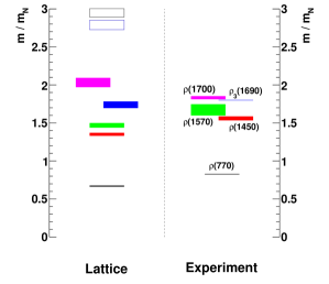
Figure 7: (Left) Masses, as ratios of the nucleon mass, of the dominant finite-volume isovector $T^{+}_{1u}$ stationary states expected to evolve into the single-meson resonances in infinite volume, computed using our $56\times 56$ correlation matrix for the $(24^{3}|390)$ ensemble. The vertical thickness of each box indicates its statistical uncertainty. The hollow boxes at the top show higher-lying states that we extract with less certainty due to the expected presence of lower-lying two-meson states that have not been taken into account. (Right) Masses of the experimentally-known spin-1 and spin-3 resonances in this energy range. Vertical thickness indicates experimental error.

The first plot shows that the lowest-lying SH-optimized operator produces level 0 and very little else. Hence, we identify level 0 with the lowest-lying resonance precursor state, expected to be the $\rho(770)$. The second plot shows that this operator produces mainly level 8, but the overlaps onto a few other states are nonnegligible. Hence, we identify level 8 as the dominant state that is the precursor of the first-excited resonance in this channel, expected to be the $\rho(1450)$. Note that the energy of level 8 is $0.3092(33)a_{t}^{-1}$, which is close to the energies of the other levels with nonnegligible overlap, so identifying this energy value with the $\rho(1450)$ is reasonable. Similarly, we identify levels 13, 31, 40, and 46 as dominantly produced by our SH-optimized operators. To help with identification, we have devised a few operators whose classical small-$a$ expansions have no contribution from spin-1; in other words, these operators should produce states dominated by spin-3 (radiative corrections could introduce $J=1$ components, but we expect these to be suppressed). We plan to use such operators to help confirm that level 31 is the precursor state corresponding to the spin-3 $\rho_{3}(1690)$.

Using the energies of levels 0, 8, 31, 40, and 46, we summarize our single-hadron spectrum (the eigenstates dominated by the resonance precursor states) in Fig. 7. This figure shows the masses as a ratio of the nucleon mass. Given that our pion mass is around 390 MeV and that our states are extracted in finite volume, precise agreement with experiment is certainly not expected. However, the general pattern of states is well reproduced. We believe we have extracted all two-meson states that lie in the range of the lowest-lying five single-hadron states. We also find two more higher lying states that couple mainly to single-hadron operators (indicated by the hollow boxes), but there are two-meson states lying below these that have not been taken into account, so we view their extractions as particularly tentative. Again, we mention that three and four meson states are not taken into account at all.

5 Conclusion

In this talk and accompanying poster, our progress in computing the finite-volume stationary-state energies of QCD was described. Our first results in the zero-momentum bosonic $I=1,\ S=0,\ T_{1u}^{+}$ symmetry sector of QCD using a correlation matrix of 56 operators were presented. In addition to a dozen spatially-extended meson operators, an unprecedented number of 44 two-meson operators were used, involving a wide variety of light isovector, isoscalar, and strange meson operators of varying relative momenta. All needed Wick contractions were efficiently evaluated using the stochastic LapH method. Issues related to level identification were discussed.

These first results are very encouraging, and preliminary results for the $(32^{3}|240)$ ensemble look even more promising, but further work is needed to finalize the spectrum in this channel. Of course, there are many other symmetry channels to investigate, which we plan to do in the near future. This work was supported by the U.S. NSF under awards PHY-0510020, PHY-0653315, PHY-0704171, PHY-0969863, and PHY-0970137, and through TeraGrid/XSEDE resources provided by TACC and NICS under grant numbers TG-PHY100027 and TG-MCA075017.

References

- [1] S. Basak, R.G. Edwards, G.T. Fleming, U.M. Heller, C. Morningstar, D. Richards, I. Sato, S. Wallace, Phys. Rev. D 72, 094506 (2005).
- [2] S. Basak, R. Edwards, G. Fleming, U.M. Heller, C. Morningstar, D. Richards, I. Sato, S. Wallace, Phys. Rev. D 72, 074501 (2005).
- [3] S. Basak, R.G. Edwards, G.T. Fleming, K.J. Juge, A. Lichtl, C. Morningstar, D.G. Richards, I. Sato, S.J. Wallace, Phys. Rev. D 76, 074504 (2007).
- [4] J. Bulava, R.G. Edwards, E. Engelson, J. Foley, B. Joo, A. Lichtl, H.W. Lin, N. Mathur, C. Morningstar, D.G. Richards, S. Wallace, Phys. Rev. D 79, 034505 (2009).
- [5] J. Bulava, R.G. Edwards, E. Engelson, B. Joo, H-W. Lin, C. Morningstar, D.G. Richards, S.J. Wallace, Phys. Rev. D 82, 014507 (2010).
- [6] C. Morningstar, J. Bulava, J. Foley, K.J. Juge, D. Lenkner, M. Peardon, C.H. Wong, Phys. Rev. D 83, 114505 (2011).
- [7] C. Morningstar, J. Bulava, B. Fahy, J. Foley, Y.C. Jhang, K.J. Juge, D. Lenkner, C.H. Wong, Phys. Rev. D 88, 014511 (2013).
- [8] C. Morningstar and M. J. Peardon, Phys. Rev. D 69, 054501 (2004).
- [9] M. Peardon, J. Bulava, J. Foley, C. Morningstar, J. Dudek, R. Edwards, B. Joo, H-W. Lin, D. Richards, K.J. Juge, Phys. Rev. D 80, 054506 (2009).
- [10] M. A. Clark, A. D. Kennedy, and Z. Sroczynski, Nucl. Phys. B (Proc. Suppl.) 140, 835 (2005).
- [11] H.-W. Lin, S. Cohen, J. Dudek, R.G. Edwards, B. Joo, D.G. Richards, J. Bulava, J. Foley, C. Morningstar, E. Engelson, S. Wallace, K.J. Juge, N. Mathur, M. Peardon, S. Ryan, Phys. Rev. D 79, 034502 (2009).